6.435 Lecture 1 v - MIT OpenCourseWare · solution? Persistency of excitation! •Note that you get...
39
System Identification 6.435 SET 3 – Nonparametric Identification Munther A. Dahleh Lecture 3 6.435, System Identification Prof. Munther A. Dahleh 1
Transcript of 6.435 Lecture 1 v - MIT OpenCourseWare · solution? Persistency of excitation! •Note that you get...

System Identification
6.435
SET 3
– Nonparametric Identification
Munther A. Dahleh
Lecture 3 6.435, System Identification Prof. Munther A. Dahleh
1
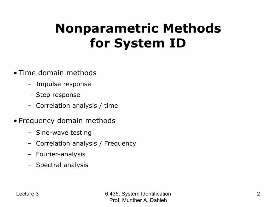
Nonparametric Methodsfor System ID
• Time domain methods
– Impulse response
– Step response
– Correlation analysis / time
• Frequency domain methods
– Sine-wave testing
– Correlation analysis / Frequency
– Fourier-analysis
– Spectral analysis
Lecture 3 6.435, System Identification Prof. Munther A. Dahleh
2

Problem Formulation
Lecture 3 6.435, System Identification Prof. Munther A. Dahleh
3
• Actual system is Linear time-invariant stable.
• Time domain methods ⇒ estimates of
Black Box
• Process:
• Frequency-domain methods ⇒ estimates of
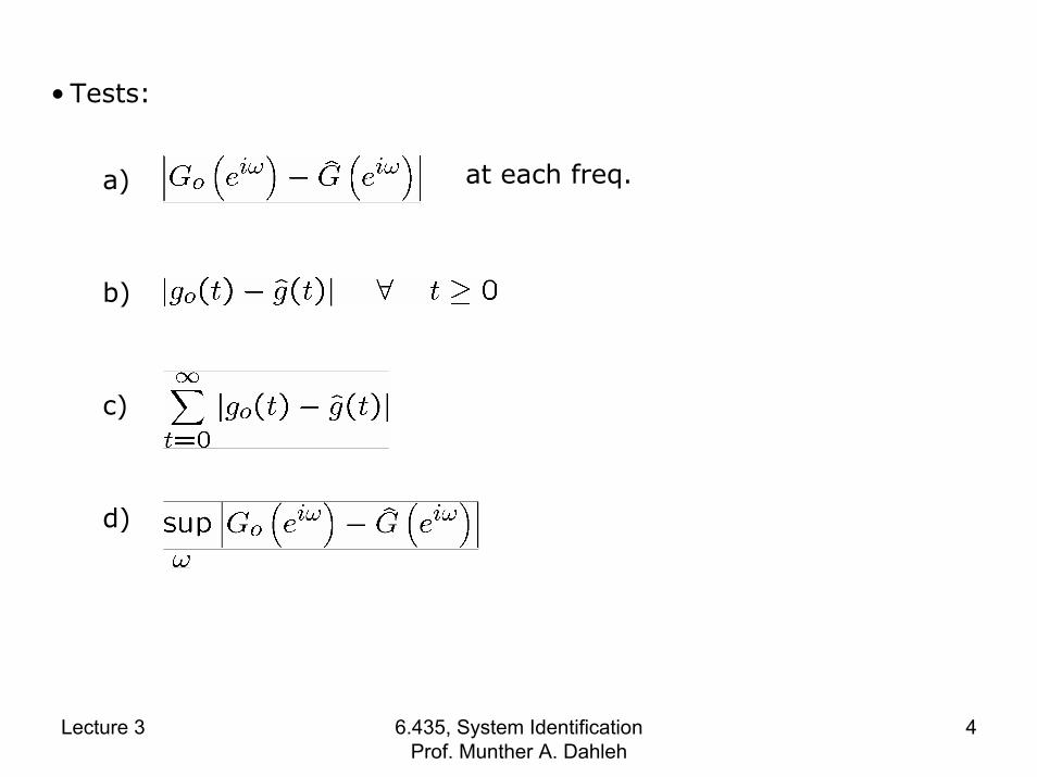
• Tests:
at each freq.a)
b)
c)
d)
Lecture 3 6.435, System Identification Prof. Munther A. Dahleh
4
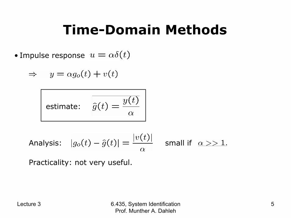
Time-Domain Methods
• Impulse response
estimate:
Analysis: small if
Practicality: not very useful.
Lecture 3 6.435, System Identification Prof. Munther A. Dahleh
5

• Step response
estimate:
Analysis:
Practicality: Not good for determining . Good for determining delays, modes….
Lecture 3 6.435, System Identification Prof. Munther A. Dahleh
6
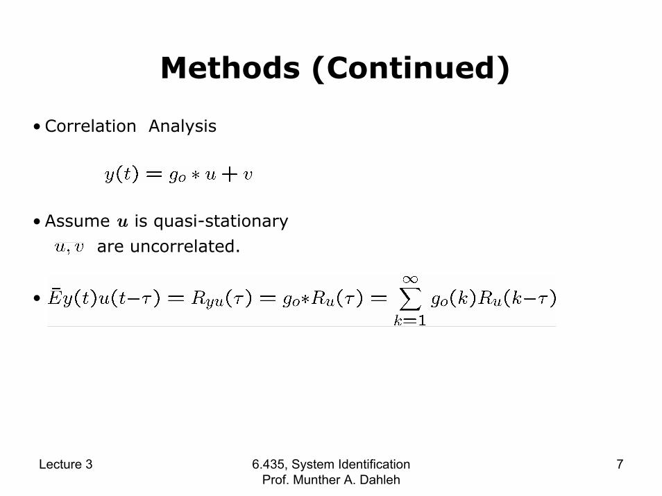
Methods (Continued)
• Correlation Analysis
• Assume u is quasi-stationary
are uncorrelated.
•
Lecture 3 6.435, System Identification Prof. Munther A. Dahleh
7
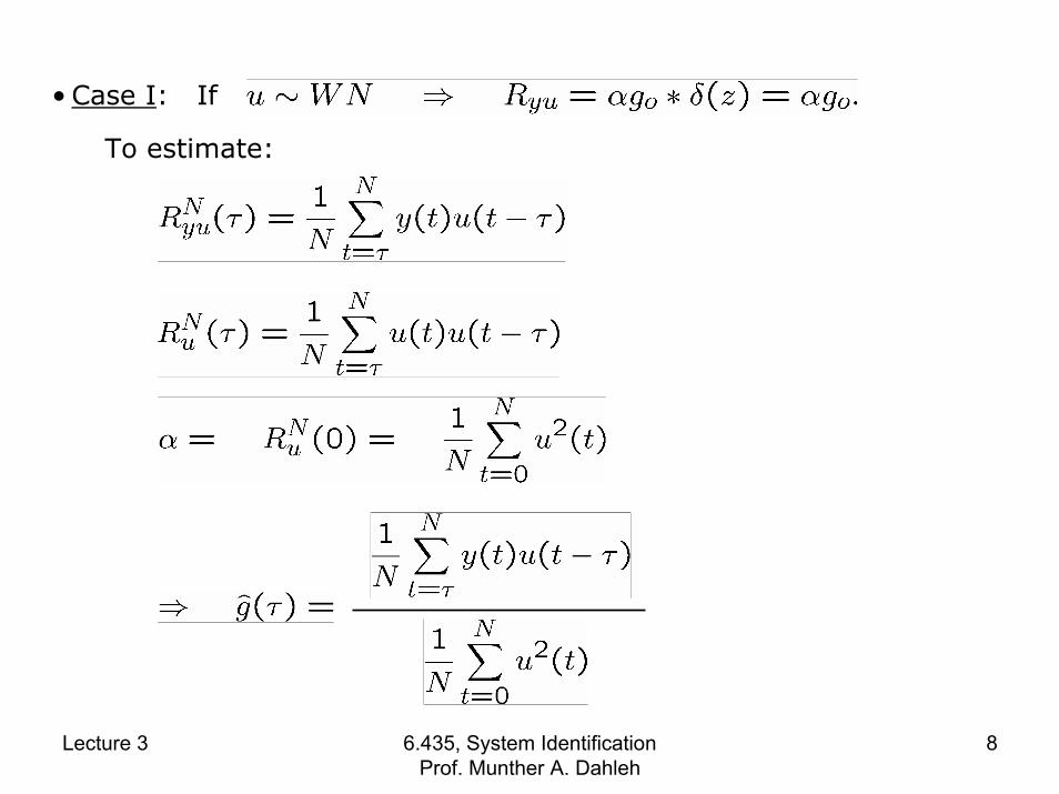
• Case I: If
To estimate:
Lecture 3 6.435, System Identification Prof. Munther A. Dahleh
8

• Case II: Input is not white.
Using the approximation
In matrix form:
notice
Lecture 3 6.435, System Identification Prof. Munther A. Dahleh
9

⇒ Estimate
• Question: Under what conditions the above system has a unique solution? Persistency of excitation!
• Note that you get the same estimate regardless of the spectrum of the noise.
Lecture 3 6.435, System Identification Prof. Munther A. Dahleh
10
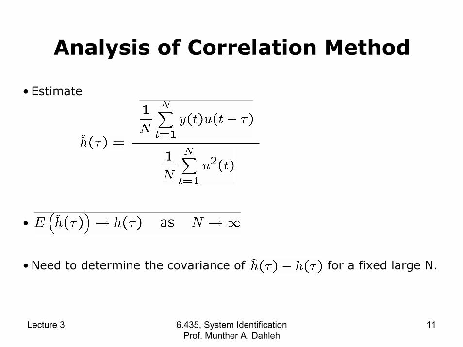
Analysis of Correlation Method
• Estimate
•
• Need to determine the covariance of for a fixed large N.
Lecture 3 6.435, System Identification Prof. Munther A. Dahleh
11
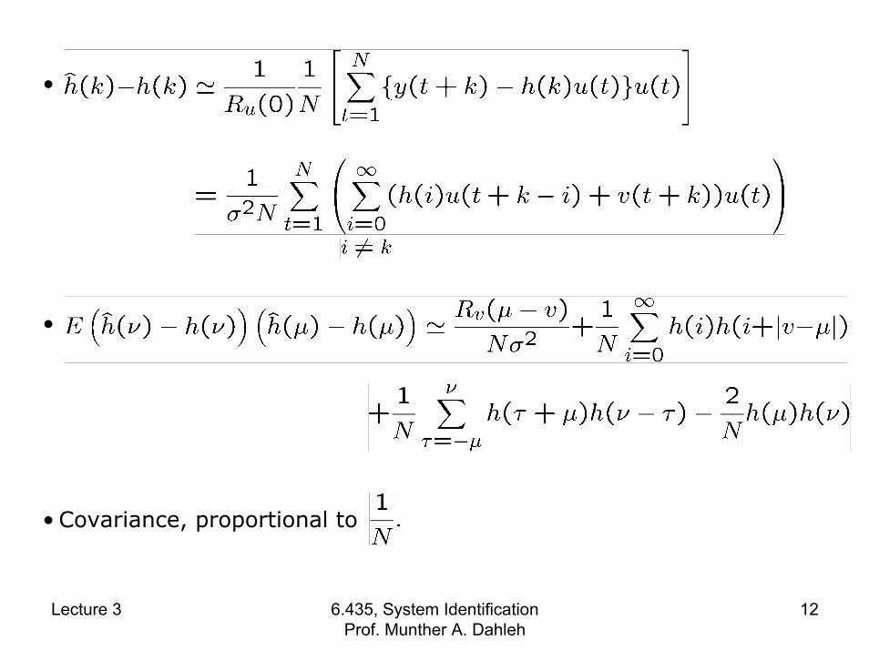
•
•
• Covariance, proportional to
Lecture 3 6.435, System Identification Prof. Munther A. Dahleh
12

Frequency-Response Analysis
• Input
• Extract
• How do you measure in the presence of noise? A good approach is correlation.
Lecture 3 6.435, System Identification Prof. Munther A. Dahleh
13
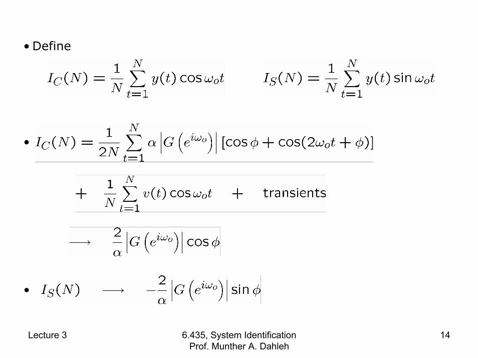
• Define
•
•
Lecture 3 6.435, System Identification Prof. Munther A. Dahleh
14

• Estimate:
• Comment:
Lecture 3 6.435, System Identification Prof. Munther A. Dahleh
15
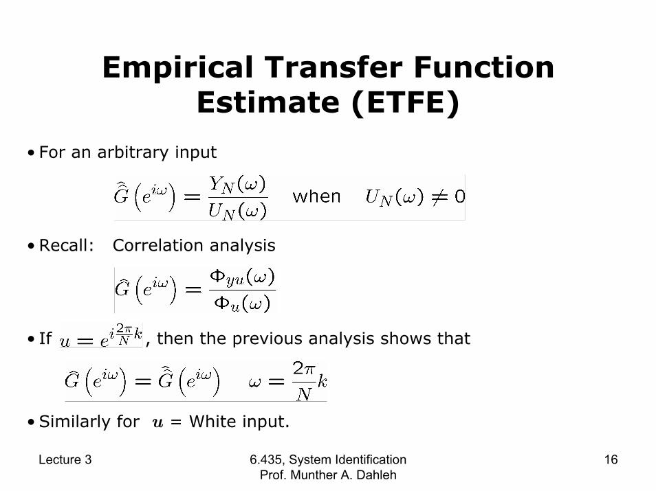
Empirical Transfer Function Estimate (ETFE)
• For an arbitrary input
• Recall: Correlation analysis
• If , then the previous analysis shows that
• Similarly for u = White input.
Lecture 3 6.435, System Identification Prof. Munther A. Dahleh
16

• General Procedure
1. Calculate
2. Obtain the inverse DFT:
3. Define
• The algorithm is quite efficient; requires only the computation of the Inverse DFT. Note also that the algorithm is Linear.
Lecture 3 6.435, System Identification Prof. Munther A. Dahleh
17
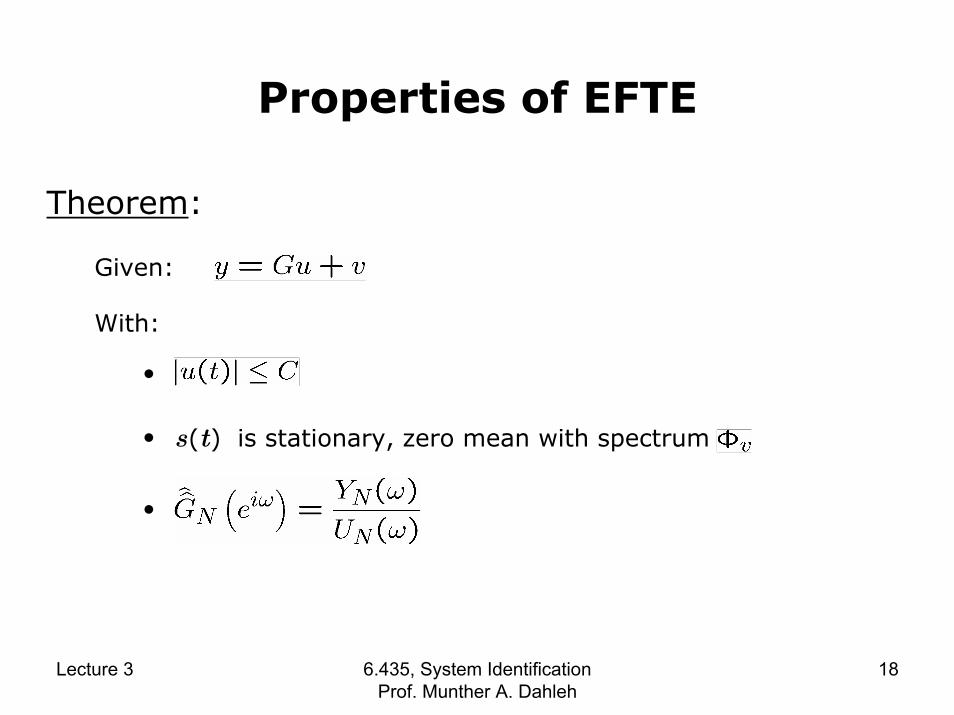
Properties of EFTE
Theorem:
Given:
With:
•
• s(t) is stationary, zero mean with spectrum
•
Lecture 3 6.435, System Identification Prof. Munther A. Dahleh
18

Then:
1.
2.
Lecture 3 6.435, System Identification Prof. Munther A. Dahleh
19
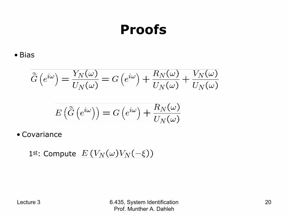
Proofs
• Bias
• Covariance
1st: Compute
Lecture 3 6.435, System Identification Prof. Munther A. Dahleh
20

Lecture 3 6.435, System Identification Prof. Munther A. Dahleh
21
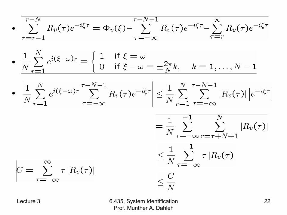
•
•
•
Lecture 3 6.435, System Identification Prof. Munther A. Dahleh
22
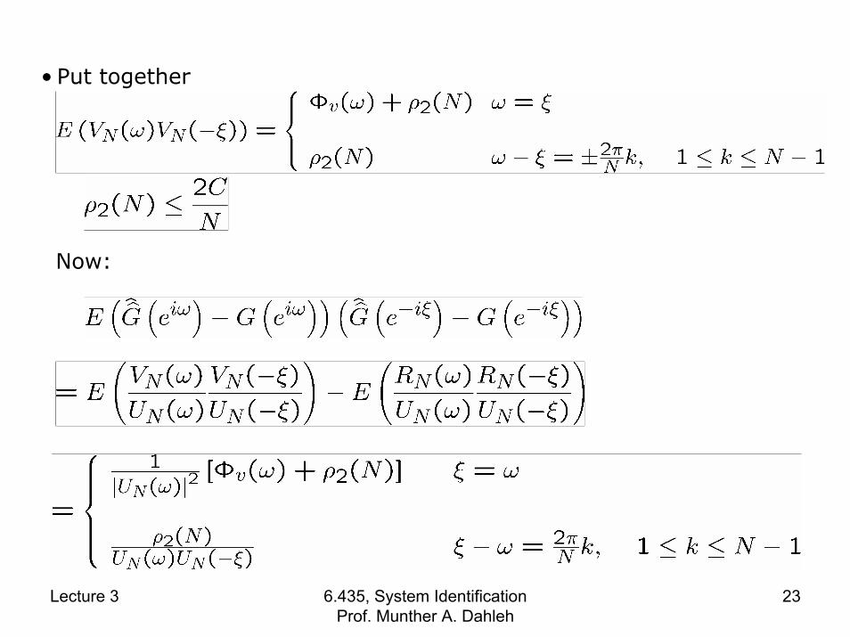
• Put together
Now:
Lecture 3 6.435, System Identification Prof. Munther A. Dahleh
23
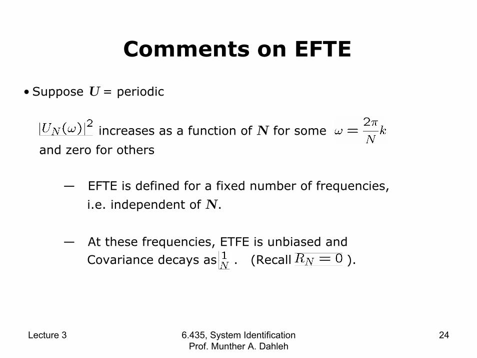
Comments on EFTE
• Suppose U = periodic
increases as a function of N for some
and zero for others
— EFTE is defined for a fixed number of frequencies,
i.e. independent of N.
— At these frequencies, ETFE is unbiased and Covariance decays as . (Recall ).
Lecture 3 6.435, System Identification Prof. Munther A. Dahleh
24

• Suppose V is a stochastic process, uncorrelated with v
in dist. (a bounded function)
– ETFE is asymptotically unbiased, with increasingly more well-defined frequencies (as N → ∞).
– The variance does not decrease as N → ∞.
– Estimates are asymptotically uncorrelated.
Lecture 3 6.435, System Identification Prof. Munther A. Dahleh
25
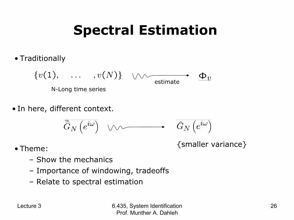
Spectral Estimation
• Traditionally
estimateN-Long time series
• In here, different context.
{smaller variance}• Theme:– Show the mechanics– Importance of windowing, tradeoffs – Relate to spectral estimation
Lecture 3 6.435, System Identification Prof. Munther A. Dahleh
26

Spectral Estimation: Non Std (Ljung)
• Idea: the actual function is smooth. The values of should be related for small intervals ω.
• According to previous analysis, is uncorrelated with and has variance
• Suppose satisfies
Lecture 3 6.435, System Identification Prof. Munther A. Dahleh
27
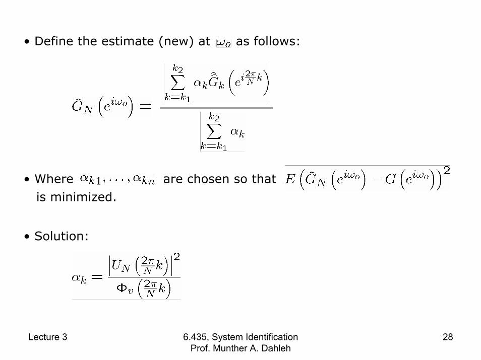
• Define the estimate (new) at as follows:
• Where are chosen so thatis minimized.
• Solution:
Lecture 3 6.435, System Identification Prof. Munther A. Dahleh
28
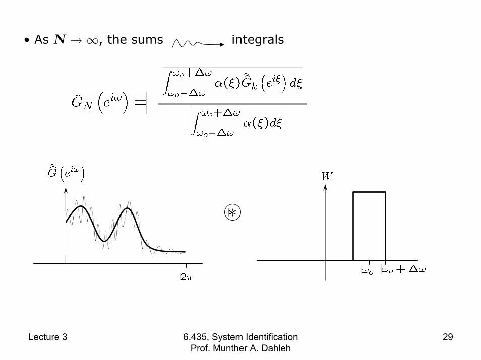
• As N → ∞, the sums integrals
Lecture 3 6.435, System Identification Prof. Munther A. Dahleh
29
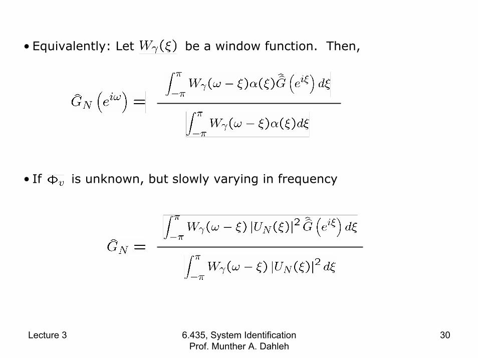
• Equivalently: Let be a window function. Then,
• If is unknown, but slowly varying in frequency
Lecture 3 6.435, System Identification Prof. Munther A. Dahleh
30
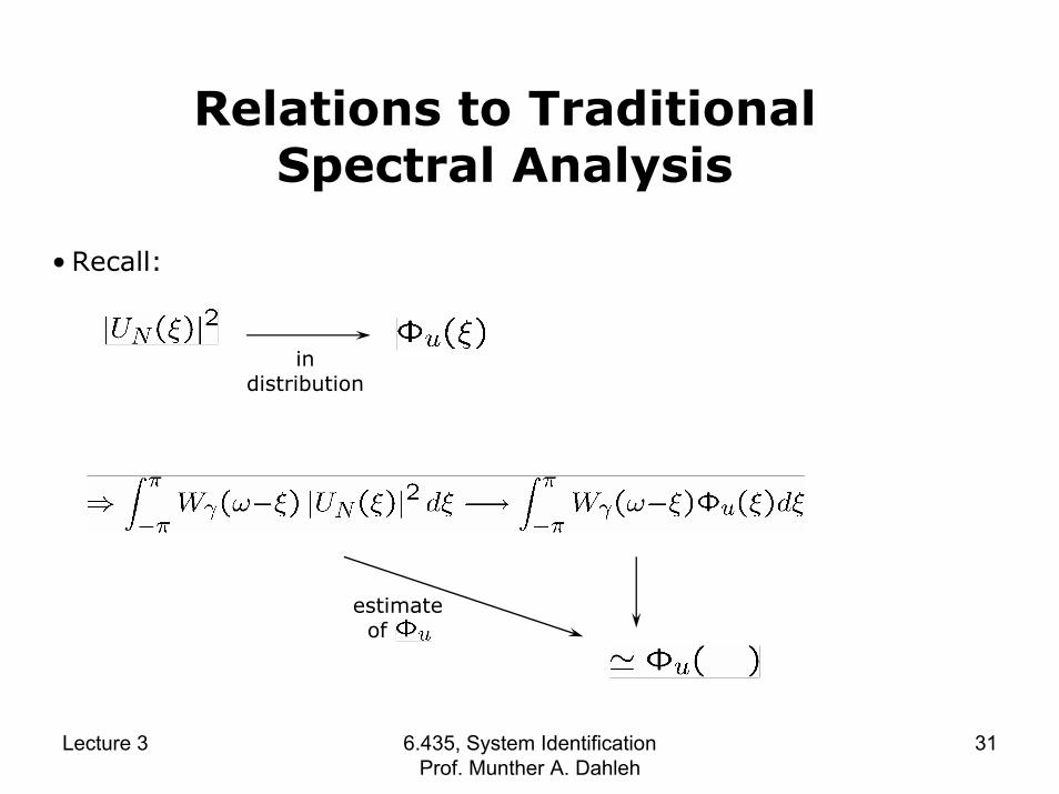
Relations to TraditionalSpectral Analysis
• Recall:
indistribution
estimate of
Lecture 3 6.435, System Identification Prof. Munther A. Dahleh
31

• Define:
•
Similarly:
• Conclusion
Lecture 3 6.435, System Identification Prof. Munther A. Dahleh
32

Efficient Computation
•
Of course for large enough but not as large
as N. Example is:
(Bartlett)
• Similarly for
Lecture 3 6.435, System Identification Prof. Munther A. Dahleh
33
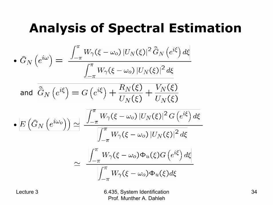
Analysis of Spectral Estimation
•
and
•
Lecture 3 6.435, System Identification Prof. Munther A. Dahleh
34
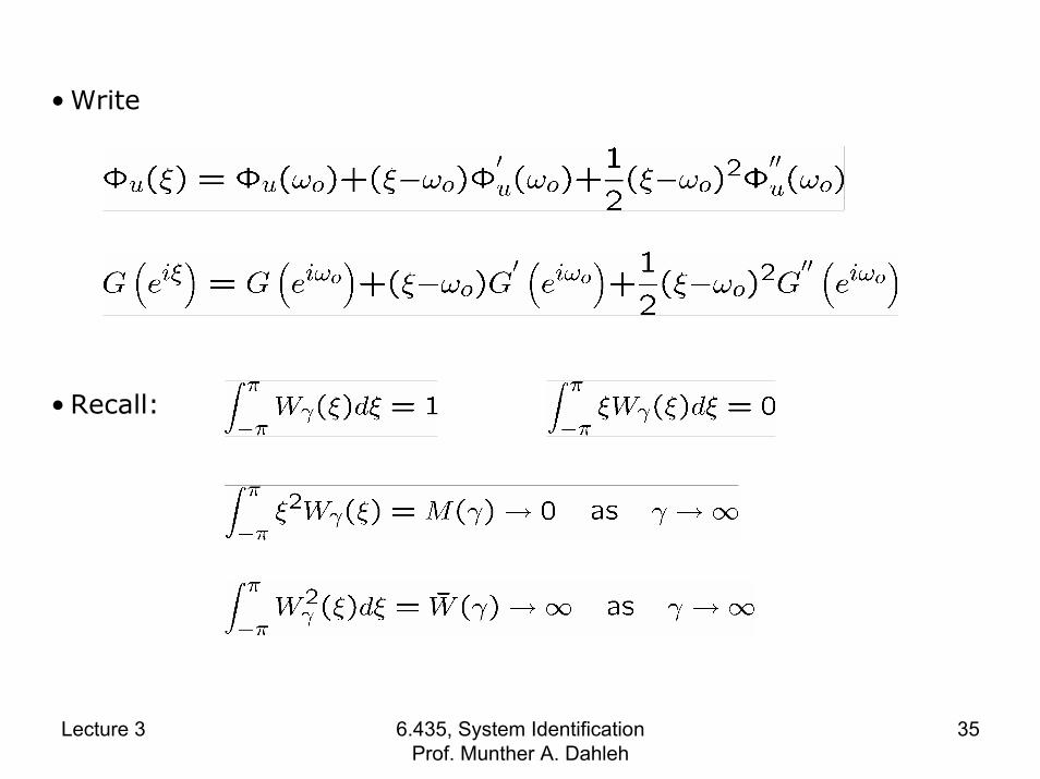
• Write
• Recall:
Lecture 3 6.435, System Identification Prof. Munther A. Dahleh
35
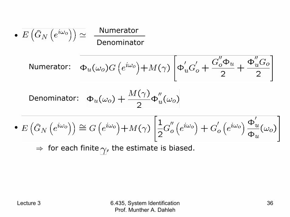
Numerator•
Denominator
Numerator:
Denominator:
•
⇒ for each finite , the estimate is biased.
Lecture 3 6.435, System Identification Prof. Munther A. Dahleh
36
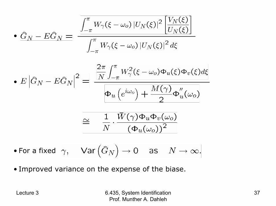
•
•
• For a fixed
• Improved variance on the expense of the biase.
Lecture 3 6.435, System Identification Prof. Munther A. Dahleh
37
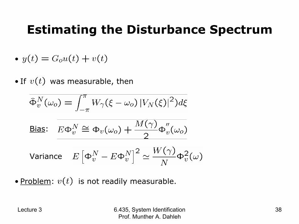
Estimating the Disturbance Spectrum
•
• If was measurable, then
Bias:
Variance
• Problem: is not readily measurable.
Lecture 3 6.435, System Identification Prof. Munther A. Dahleh
38
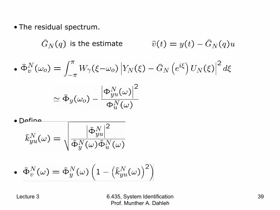
• The residual spectrum.
is the estimate
•
• Define
•
Lecture 3 6.435, System Identification Prof. Munther A. Dahleh
39