6.3 Probabilities with Large Numbers - University of...
33
1 6.3 Probabilities with Large Numbers ! In general, we can’t perfectly predict any single outcome when there are numerous things that could happen. ! But, when we repeatedly observe many observations , we expect the distribution of the observed outcomes to show some type of pattern or regularity.
Transcript of 6.3 Probabilities with Large Numbers - University of...

1
6.3 Probabilities with Large Numbers
! In general, we can’t perfectly predict any single outcome when there are numerous things that could happen.
! But, when we repeatedly observe many observations, we expect the distribution of the observed outcomes to show some type of pattern or regularity.

2
Tossing a coin
! One flip " It’s a 50-50 chance whether it’s a head or tail.
! 100 flips " I can’t predict perfectly, but I’m not going to
predict 0 tails, that’s just not likely to happen. " I’m going to predict something close to 50 tails
and 50 heads. That’s much more likely than 0 tails or 0 heads.

3
Tossing a coin many times
! Let represent the proportion of heads that I get when I toss a coin many times.
" If I toss 45 heads on 100 flips, then
" is pronounced “p-hat”. It is the relative frequency of heads in this example.
" If I toss 48 heads on 100 flips, then
p̂
p̂ = 45100
= 0.45
p̂ = 48100
= 0.48
p̂

4
Tossing a coin many times
! I expect (the proportion of heads) to be somewhere near 50% or 0.50.
! What if I only toss a coin two times? " The only possible values for are…
! 1) = 0/2 = 0.00 ! 2) = 1/2 = 0.50 ! 3) = 2/2 = 1.00
p̂
p̂p̂p̂p̂
Pretty far from the true probability of flipping a head on a fair coin (0.5).
5
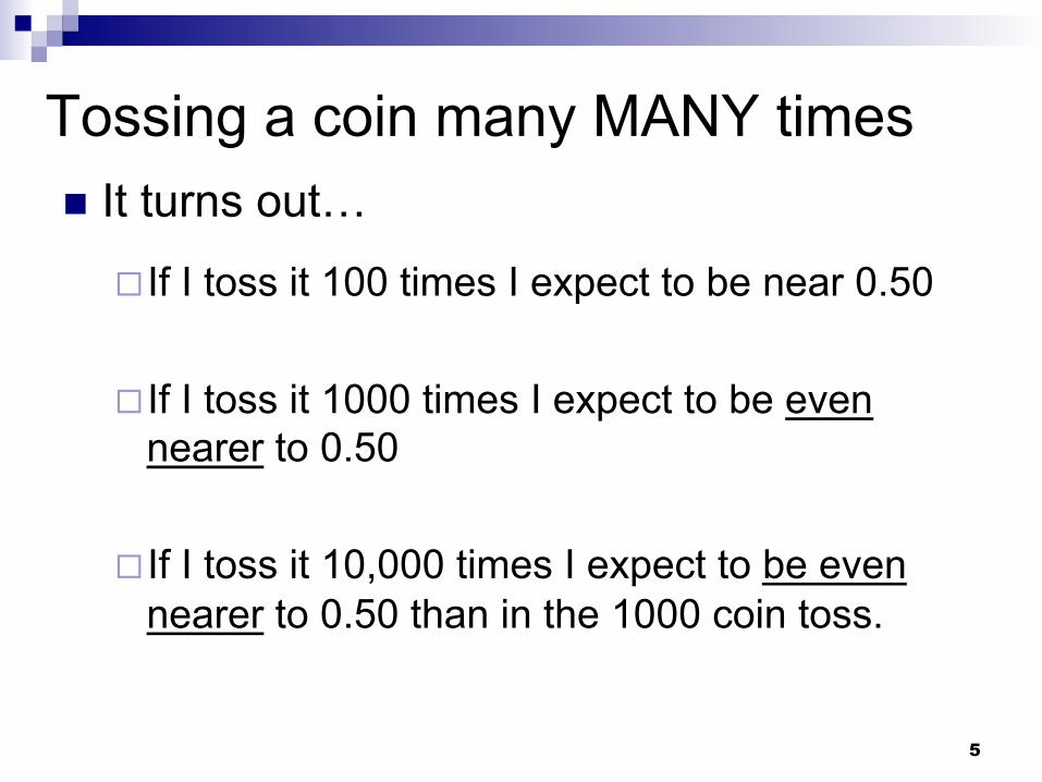
Tossing a coin many MANY times ! It turns out…
" If I toss it 100 times I expect to be near 0.50
" If I toss it 1000 times I expect to be even nearer to 0.50
" If I toss it 10,000 times I expect to be even nearer to 0.50 than in the 1000 coin toss.

6
Tossing a coin many MANY times ! This shows a very possible observed
situation…
" Toss it 100 times, 45 heads.
" Toss it 1000 times, 485 heads.
" Toss it 10,000 times, 4955 heads.
p̂ = 4851000
= 0.4850
p̂ = 45100
= 0.4500
p̂ = 495510000
= 0.4955
! With more tosses, the closer gets to the truth of 0.50 (it’s “zero-ing in” on the truth).
p̂

7 7
Law of Large Numbers ! For repeated independent trials, the long run
(i.e. after many many trials) relative frequency of an outcome gets closer and closer to the true probability of the outcome.
" If you’re using your trials to estimate a probability (i.e. empirical probability), you’ll do a better job at estimating by using a larger number of trials.

Computer simulation of rolling a die. We’ll keep track of the proportion of 1’s.
8
Number of rolls getting larger #

9 9
Law of Large Numbers ! Suppose you don’t know if a coin is fair.
" Let represent the true probability of a head. from n=10 trials
is an OK estimate for .
from n=1000 trials is a better estimate for .
from n=10,000 trials is an even better estimate for .
p̂
p̂
p̂p
p
p
60.0106ˆ ==p
513.01000513ˆ ==p
p̂ = 501410000
= 0.5014
p

$ In the coin flip example, your estimate with n=10 may hit the truth right on the nose, but you have a better chance of being very close to when you have a much larger n.
10 10
Law of Large Numbers (LLN)
5.0=pp̂

11 11
! LLN let’s insurance companies do a pretty good job of estimating costs in the coming year for large groups (i.e. when they have LOTS and LOTS of insurees).
" Hard to predict for one person, but we can do a pretty good job of predicting total costs or total proportion of people who will have an accident for a group.
Law of Large Numbers (LLN)

Example: ! The Binary Computer Company
manufactures computer chips used in DVD players. Those chips are made with 0.73 defective rate.
" A) When one chip is drawn, list the possible outcomes.
" B) If one chip is randomly selected, find the probability that it is good.
" C) If you select 100,000 chips, how many defects should you expect?
12

" A) Two possible outcomes: defective or good.
" B) P(good)=1-P(defective) = 1-0.73=0.27
" C) If you select 100,000 chips, how many defects should you expect? ! As the number of chips sampled gets larger, the
proportion of defects in the sample approaches the true proportion of defects (which is 0.73). So, with this large of a sample, I would expect about 73% of the sample to be defects, or 0.73 x 100,000= 73,000.
! I used the Law of Large numbers in the above. 13
Answers:

Expected Value ! Game based on the roll a die:
" If a 1 or 2 is thrown, the player gets $3. If a 3, 4, 5, or 6 is thrown, the house wins (you get nothing).
" Would you play if it cost $5 to join the game?
" Would you play if it cost $1 to join the game?
" What do you EXPECT to gain (or lose) from playing?
14 We’ll return to this example later…

Expected Value ! There are alternative ways to compute
expected values (all with the same result). I will focus on those where the probabilities of the possible events sum to 1.
15

Expected Value ! Life insurance companies depend on the
law of large numbers to stay solvent (i.e. be able to pay their debts).
! I pay $1000 annually for life insurance for a $500,000 policy (in the event of a death).
! Suppose they only insured me. " If I live (high probability), they make $1000. " If I die (low probability), they lose $499,000!!
! Should they gamble that I’m not going to die? Not sound business practice.
16

Expected Value ! It’s hard to predict the outcome for one
person, but much easier to predict the ‘average’ of outcomes among a group of people.
! Insurance is based on the probability of events (death, accidents, etc.), some of which are very unlikely.
17

Expected Value ! For the upcoming year, suppose:
" P(die) = 1/500 = 0.002 " P(live) = 499/500 = 0.998 " A life insurance policy costs $100 and pays
out $10,000 in the event of a death
! If the company insures a million people, what do they expect to gain (or lose)?
18

Expected Value ! For each policy, one of two things can
happen… a payout (die) or no payout (live). " If the person dies and they pay out, they
lose $9,900 on the policy. (they did collect the $100 regardless of death or not)
" If the person lives and there’s no payout, they gain $100 on the policy.
19
Expected Value = (1/500)*(-$9,900)+(499/500)*($100) = $80 (per policy)
This amounts to a profit of $80,000,000 on sales of 1 million policies

Expected Value (per policy)
20
Expected Value = (1/500)*(-$9,900)+(499/500)*($100) = $80 (per policy)
This amounts to a profit of $80,000,000 on sales of 1 million policies (overall expected value of $80,000,000).
The negative
loss
The positive
gain
Probability of a loss
Probability of a gain

Expected Value ! For the upcoming year, suppose:
" P(die) = 1/500 = 0.002 " P(live) = 499/500 = 0.998 " A life insurance policy costs $1000 and pays
out $500,000 in the event of a death
21
Expected Value = (1/500)*(-$499,000)+(499/500)*($1000) = $0 (per policy)
They expect to just ‘break even’ (if more people die than expected, they’re in trouble). Charging any less would result in an expected loss.

Expected Value ! The law of large numbers comes into play
for insurance companies because their actual payouts will depend on the observed number of deaths (some uncertainty).
! As they observe (or insure) more people, the relative frequency of a death will get closer and closer to the 1/500 probability on which they based their calculations.
22

23 Copyright © 2009 Pearson Education, Inc.
Calculating Expected Value Consider two events, each with its own value and probability. The expected value is
expected value = (value of event 1) * (probability of event 1) + (value of event 2) * (probability of event 2)
This formula can be extended to any number of events by including more terms in the sum.

Expected Value ! Game based on the roll a die:
" If a 1 or 2 is thrown, the player gets $3. If a 3, 4, 5, or 6 is thrown, the house wins (you get nothing).
" If the game costs $5 to play, what is the expected value of a game?
24
Expected Value = (2/6)*(-$2)+(4/6)*(-$5) = -$4 (per game)
No matter what is rolled, you’re losing money.

Expected Value ! Game based on the roll a die:
" If a 1 or 2 is thrown, the player gets $3. If a 3, 4, 5, or 6 is thrown, the house wins (you get nothing).
" If the game costs $1 to play, what is the expected value of a game?
25
Expected Value = (2/6)*($2)+(4/6)*(-$1) = $0 (per game)
This is a ‘fair game’.

26 Copyright © 2009 Pearson Education, Inc.
Expected Value
Definition The expected value of a variable is the weighted average of all its possible events. Because it is an average, we should expect to find the “expected value” only when there are a large number of events, so that the law of large numbers comes into play.
For the life insurance company, the observed relative frequency of deaths approaches the truth (which is 1/500) as they get more and more insurees.

Expected Value ! Game based on the roll of two dice:
" If a sum of 12 is thrown, the player gets $40. If anything else is thrown, the house wins (you get nothing).
" If the game costs $4 to play, what is the expected value of a game?
27
Expected Value = (1/36)*($36)+(35/36)*(-$4) = - $2.89 (per game)
This is a ‘unfair game’ (for the gambler).

28
Everyone who bets any part of his fortune, however small, on a mathematically unfair game of chance acts irrationally…
-- Daniel Bernoulli, 18th century mathematician
In the long run, you know you’ll lose. But perhaps you think you can ‘beat the house’ in the short run.

29 Copyright © 2009 Pearson Education, Inc.
The Gambler’s Fallacy
Definition The gambler’s fallacy is the mistaken belief that a streak of bad luck makes a person “due” for a streak of good luck.

! Game based on the toss of a fair coin: " Win $1 for heads and lose $1 for tails
(no cost to play).
" After playing 100 times, you have 45 heads and 55 tails (you’re down $10).
" Thinking things will ‘balance out in the end’ you keep playing until you’ve played 1000 times. Unfortunately, you now have 480 heads and 520 tails (you’re down $40).
30
Expected Value = (1/2)*($1)+(1/2)*(-$1) = $0 (per game)

! Do these results go against what we know about the law of large numbers? Nope.
" The proportion of heads DID get closer to 0.50
" But the difference between the number of heads and tails got larger, which is reasonable as the number of tosses gets larger.
31
p̂n=100 =45100
= 0.450
p̂n=1000 =4801000
= 0.480

32
Outcomesofcointossingtrials
Numberoftosses
Numberoftails
Numberofheads
Percentageofheads
Differencebetweennumberof
headsandtails100 55 45 45% 10
1000 520 480 48% 4010,000 5,050 4,950 49.50% 100
100,000 50,100 49,900 49.90% 200
! Though the percentage of heads gets closer to 50%, the difference in the number of heads and tails doesn’t get closer to zero " (and the difference is what relates to the money in
your pocket).

Streaks ! When a sequence of events gives rise to a
streak, this can also lend itself to the gambler’s fallacy. " Flip a coin 7 times: HHHHHHH " But we know that the above streak is just as
likely as HTTHTTH because these are equally likely outcomes.
" Perhaps you think a tail is ‘due’ next in the first streak, but P(tail)=P(head)=0.50 no matter what you tossed in the past.
33