04/18/23 CS194 Lecture 1

Load Balancing Part 1: Dynamic Load Balancing

Kathy Yelickyelick@cs.berkeley.edu

www.cs.berkeley.edu/~yelick/cs194f07

04/18/23 CS194 Lecture 2

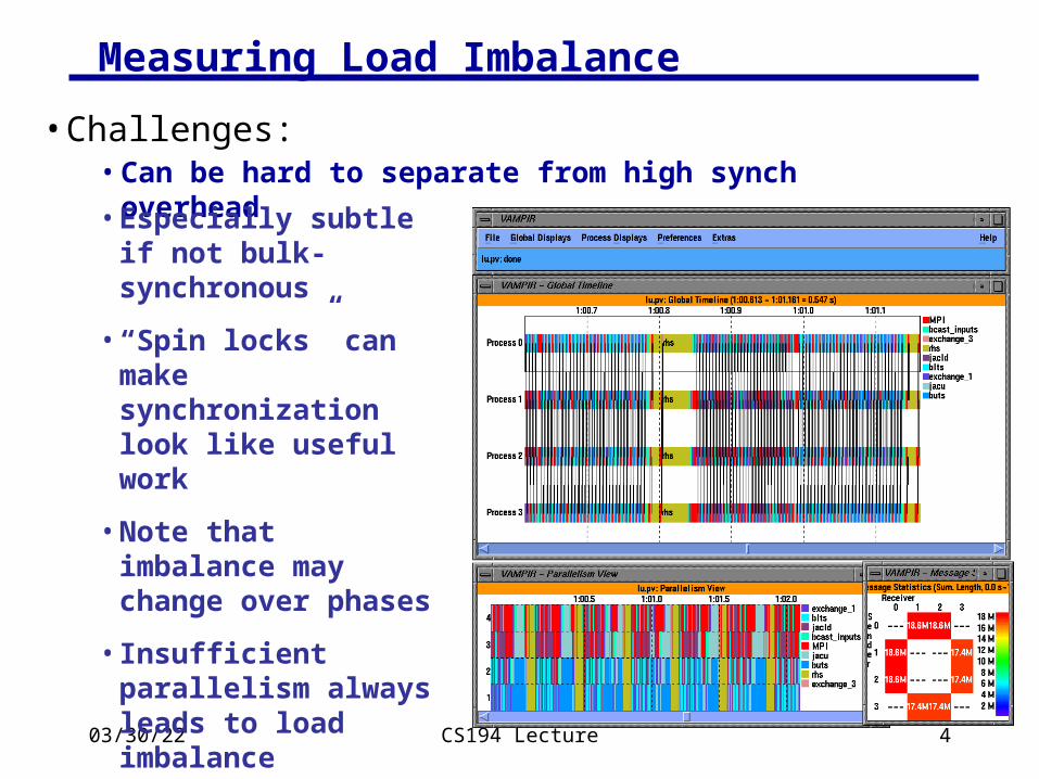
Implementing Data Parallelism

• Why didn’t data parallel languages like NESL, *LISP, pC++, HPF, ZPL take over the world in the last decade?

• 1) parallel machines are made from commodity processors, not 1-bit processors; the compilation problem is nontrivial (not necessarily impossible) and users were impatient

logical execution of statement mapping to bulk- synchronous execution

• 2) data parallelism is not a good model when the code has lots of branches (recall “turn off processors” model)

04/18/23 CS194 Lecture 3

Load Imbalance in Parallel Applications

The primary sources of inefficiency in parallel codes:• Poor single processor performance

• Typically in the memory system

• Too much parallelism overhead• Thread creation, synchronization, communication

• Load imbalance• Different amounts of work across processors

• Computation and communication

• Different speeds (or available resources) for the processors• Possibly due to load on the machine

• How to recognizing load imbalance• Time spent at synchronization is high and is uneven across

processors, but not always so simple …

04/18/23 CS194 Lecture 4

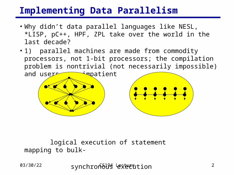
Measuring Load Imbalance

• Challenges:• Can be hard to separate from high synch overhead

• Especially subtle if not bulk-synchronous

• “Spin locks” can make synchronization look like useful work

• Note that imbalance may change over phases

• Insufficient parallelism always leads to load imbalance

• Tools like TAU can help (acts.nersc.gov)

04/18/23 CS194 Lecture 5

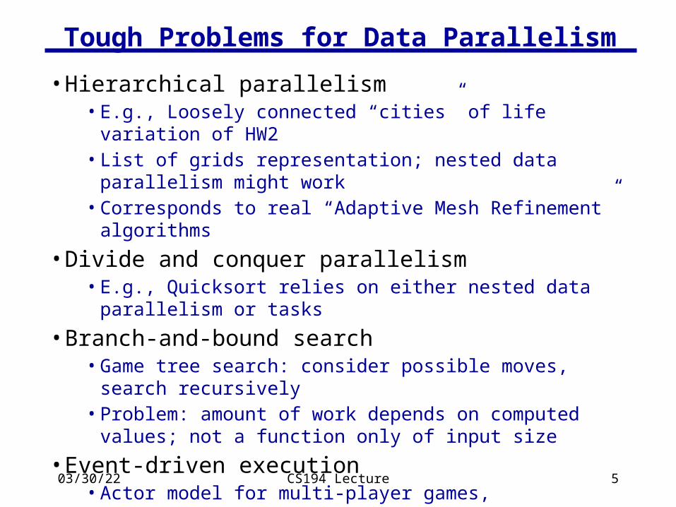
Tough Problems for Data Parallelism

• Hierarchical parallelism• E.g., Loosely connected “cities” of life variation of HW2• List of grids representation; nested data parallelism might work• Corresponds to real “Adaptive Mesh Refinement” algorithms

• Divide and conquer parallelism• E.g., Quicksort relies on either nested data parallelism or tasks

• Branch-and-bound search• Game tree search: consider possible moves, search recursively• Problem: amount of work depends on computed values; not a

function only of input size

• Event-driven execution• Actor model for multi-player games, asynchronous circuit

simulation, etc.

Load balancing is a significant problem for all of these

04/18/23 CS194 Lecture 6

Load Balancing Overview

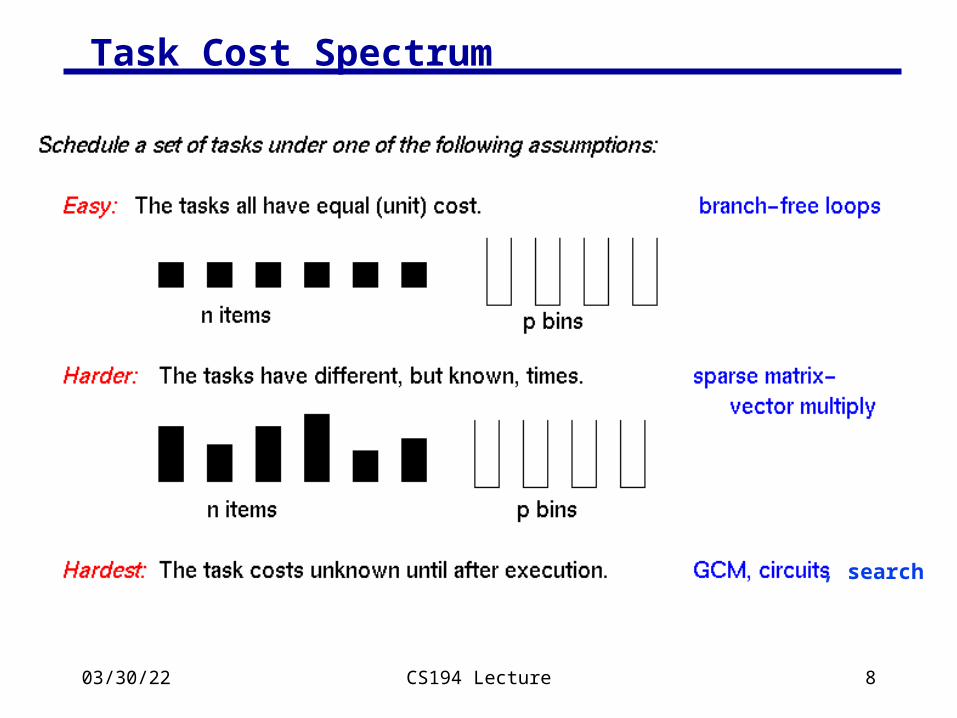
Load balancing differs with properties of the tasks (chunks of work):

• Tasks costs• Do all tasks have equal costs?• If not, when are the costs known?

• Before starting, when task created, or only when task ends

• Task dependencies• Can all tasks be run in any order (including parallel)?• If not, when are the dependencies known?

• Before starting, when task created, or only when task ends

• Locality• Is it important for some tasks to be scheduled on the same

processor (or nearby) to reduce communication cost?• When is the information about communication known?

04/18/23 CS194 Lecture 7

Outline• Motivation for Load Balancing• Recall graph partitioning as load balancing technique• Overview of load balancing problems, as determined by

• Task costs• Task dependencies• Locality needs

• Spectrum of solutions• Static - all information available before starting• Semi-Static - some info before starting• Dynamic - little or no info before starting

• Survey of solutions• How each one works• Theoretical bounds, if any• When to use it

04/18/23 CS194 Lecture 8

Task Cost Spectrum

, search

04/18/23 CS194 Lecture 9

Task Dependency Spectrum

04/18/23 CS194 Lecture 10

Task Locality Spectrum (Communication)

04/18/23 CS194 Lecture 11

Spectrum of Solutions

A key question is when certain information about the load balancing problem is known.

Many combinations of answer leads to a spectrum of solutions:

• Static scheduling. All information is available to scheduling

algorithm, which runs before any real computation starts. • Off-line algorithms make decisions before execution time

• Semi-static scheduling. Information may be known at program startup, or the beginning of each timestep, or at other well-defined points.

• Offline algorithms may be used, between major steps. • Dynamic scheduling. Information is not known until mid-

execution. • On-line algorithms make decisions mid-execution

04/18/23 CS194 Lecture 12

Dynamic Load Balancing

• Motivation for dynamic load balancing• Search algorithms as driving example

• Centralized load balancing• Overview• Special case for schedule independent loop iterations

• Distributed load balancing• Overview• Engineering• Theoretical results

• Example scheduling problem: mixed parallelism• Demonstrate use of coarse performance models

04/18/23 CS194 Lecture 13

Search

• Search problems are often:• Computationally expensive• Have very different parallelization strategies than physical

simulations.• Require dynamic load balancing

• Examples:• Optimal layout of VLSI chips• Robot motion planning• Chess and other games (N-queens)• Speech processing• Constructing phylogeny tree from set of genes

04/18/23 CS194 Lecture 14

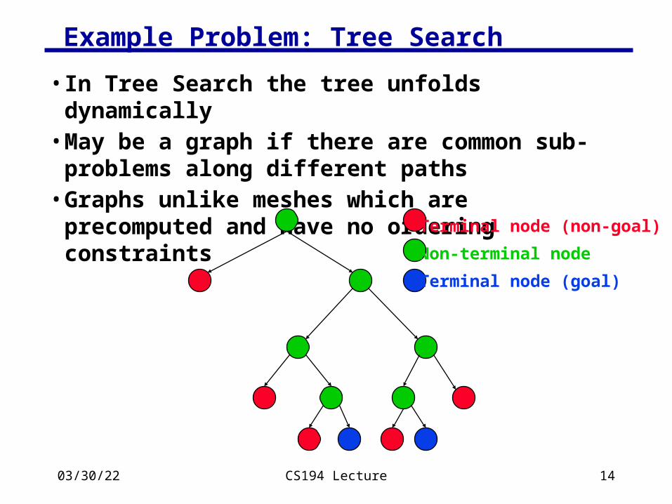
Example Problem: Tree Search

• In Tree Search the tree unfolds dynamically• May be a graph if there are common sub-problems

along different paths• Graphs unlike meshes which are precomputed and

have no ordering constraintsTerminal node (non-goal)

Non-terminal node

Terminal node (goal)

04/18/23 CS194 Lecture 15

Sequential Search Algorithms

• Depth-first search (DFS)• Simple backtracking

• Search to bottom, backing up to last choice if necessary

• Depth-first branch-and-bound• Keep track of best solution so far (“bound”)• Cut off sub-trees that are guaranteed to be worse than bound

• Iterative Deepening• Choose a bound on search depth, d and use DFS up to depth d• If no solution is found, increase d and start again• Iterative deepening A* uses a lower bound estimate of cost-to-

solution as the bound

• Breadth-first search (BFS)• Search across a given level in the tree

04/18/23 CS194 Lecture 16

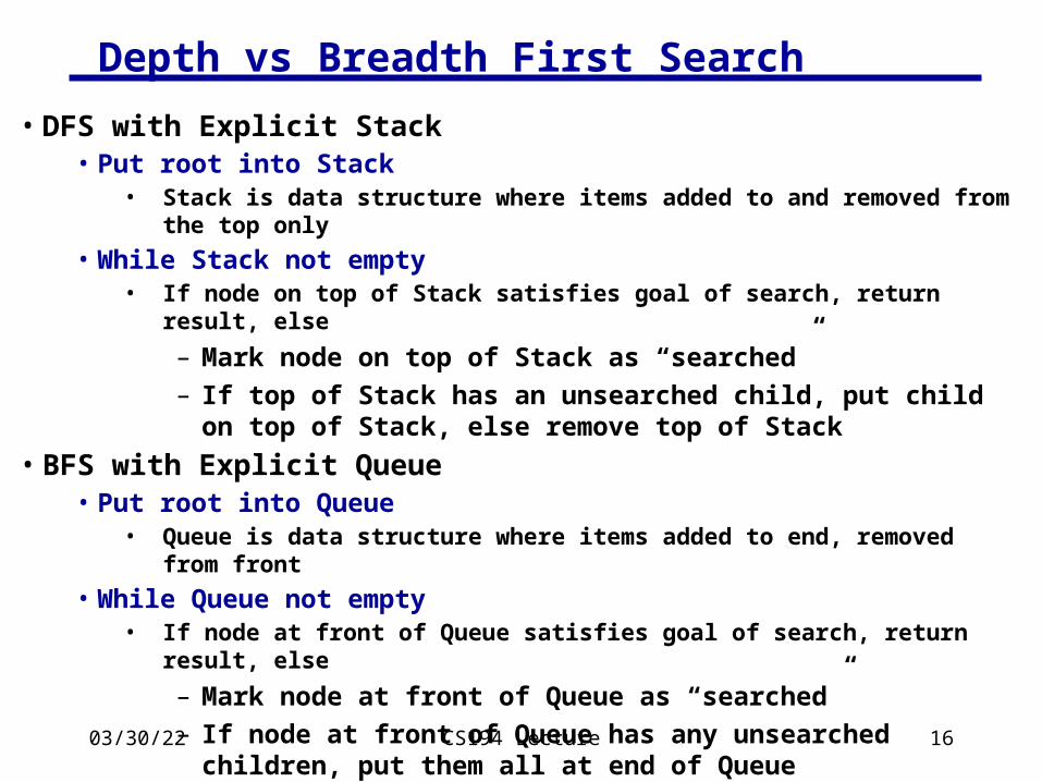
Depth vs Breadth First Search

• DFS with Explicit Stack• Put root into Stack

• Stack is data structure where items added to and removed from the top only

• While Stack not empty• If node on top of Stack satisfies goal of search, return result, else

– Mark node on top of Stack as “searched”

– If top of Stack has an unsearched child, put child on top of Stack, else remove top of Stack

• BFS with Explicit Queue• Put root into Queue

• Queue is data structure where items added to end, removed from front

• While Queue not empty• If node at front of Queue satisfies goal of search, return result, else

– Mark node at front of Queue as “searched”

– If node at front of Queue has any unsearched children, put them all at end of Queue

– Remove node at front from Queue

04/18/23 CS194 Lecture 17

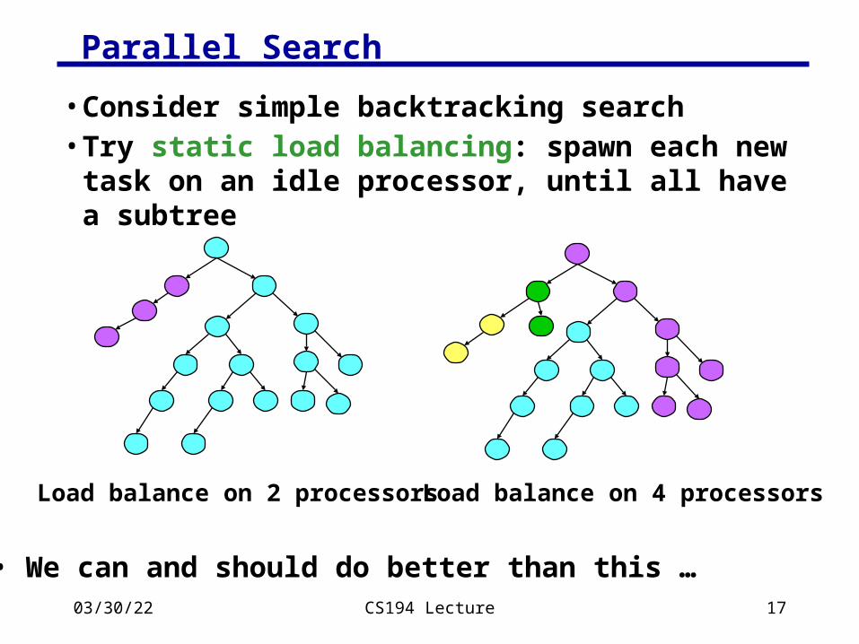
Parallel Search

• Consider simple backtracking search• Try static load balancing: spawn each new task on

an idle processor, until all have a subtree

Load balance on 2 processors Load balance on 4 processors

• We can and should do better than this …

04/18/23 CS194 Lecture 18

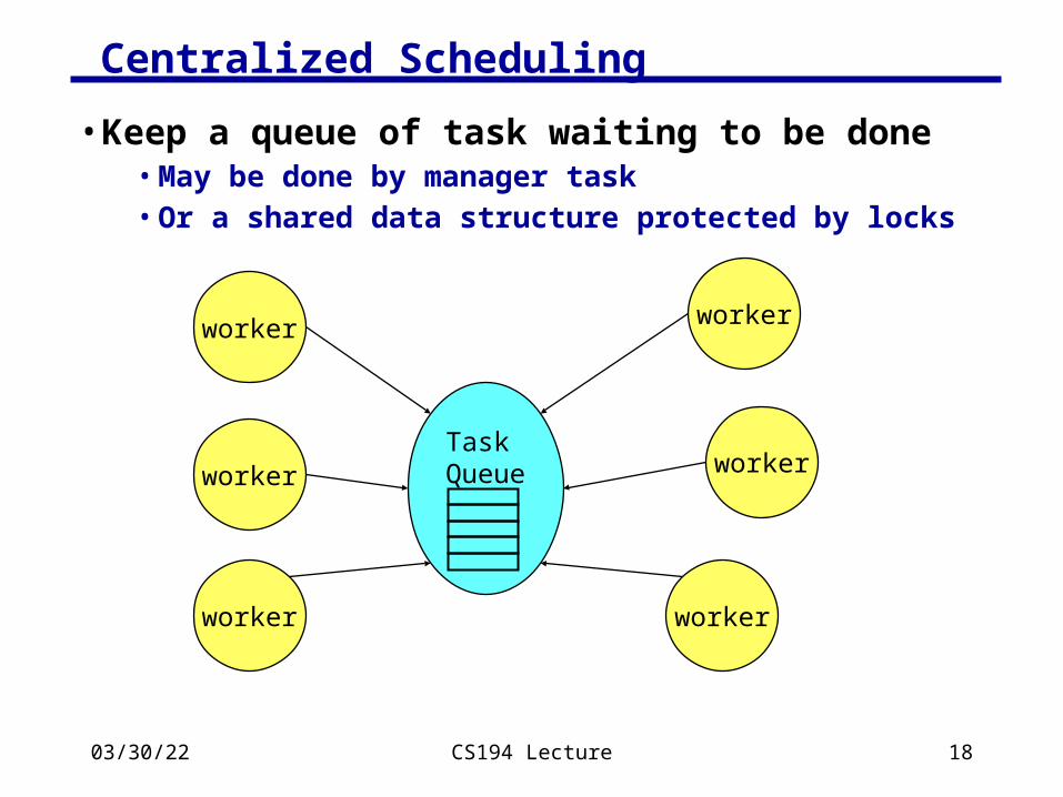
Centralized Scheduling

• Keep a queue of task waiting to be done• May be done by manager task• Or a shared data structure protected by locks

Task Queue

worker

worker

workerworker

worker

worker

04/18/23 CS194 Lecture 19

Centralized Task Queue: Scheduling Loops

• When applied to loops, often called self scheduling:• Tasks may be range of loop indices to compute• Assumes independent iterations• Loop body has unpredictable time (branches) or the problem is

not interesting

• Originally designed for:• Scheduling loops by compiler (or runtime-system)• Original paper by Tang and Yew, ICPP 1986

• This is:• Dynamic, online scheduling algorithm• Good for a small number of processors (centralized)• Special case of task graph – independent tasks, known at once

04/18/23 CS194 Lecture 20

Variations on Self-Scheduling

• Typically, don’t want to grab smallest unit of parallel work, e.g., a single iteration• Too much contention at shared queue

• Instead, choose a chunk of tasks of size K.• If K is large, access overhead for task queue is small• If K is small, we are likely to have even finish times (load

balance)

• (at least) Four Variations:1. Use a fixed chunk size2. Guided self-scheduling3. Tapering4. Weighted Factoring

04/18/23 CS194 Lecture 21

Variation 1: Fixed Chunk Size

• Kruskal and Weiss give a technique for computing the optimal chunk size

• Requires a lot of information about the problem characteristics

• e.g., task costs as well as number

• Not very useful in practice. • Task costs must be known at loop startup time• E.g., in compiler, all branches be predicted based on loop

indices and used for task cost estimates

04/18/23 CS194 Lecture 22

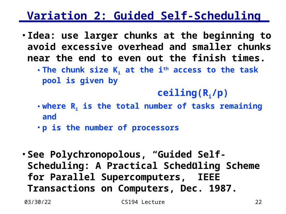
Variation 2: Guided Self-Scheduling

• Idea: use larger chunks at the beginning to avoid excessive overhead and smaller chunks near the end to even out the finish times.

• The chunk size Ki at the ith access to the task pool is given by

ceiling(Ri/p)• where Ri is the total number of tasks remaining and

• p is the number of processors

• See Polychronopolous, “Guided Self-Scheduling: A Practical Scheduling Scheme for Parallel Supercomputers,” IEEE Transactions on Computers, Dec. 1987.

04/18/23 CS194 Lecture 23

Variation 3: Tapering

• Idea: the chunk size, Ki is a function of not only the remaining work, but also the task cost variance

• variance is estimated using history information• high variance => small chunk size should be used• low variance => larger chunks OK

• See S. Lucco, “Adaptive Parallel Programs,” PhD Thesis, UCB, CSD-95-864, 1994.

• Gives analysis (based on workload distribution)• Also gives experimental results -- tapering always works

at least as well as GSS, although difference is often small

04/18/23 CS194 Lecture 24

Variation 4: Weighted Factoring

• If hardware is heterogeneous (some processors faster than others)

• Idea: similar to self-scheduling, but divide task cost by computational power of requesting node

• Also useful for shared resource clusters, e.g., built using all the machines in a building

• as with Tapering, historical information is used to predict future speed

• “speed” may depend on the other loads currently on a given processor

• See Hummel, Schmit, Uma, and Wein, SPAA ‘96• includes experimental data and analysis

04/18/23 CS194 Lecture 25

When is Self-Scheduling a Good Idea?

Useful when:

• A batch (or set) of tasks without dependencies• can also be used with dependencies, but most analysis

has only been done for task sets without dependencies

• The cost of each task is unknown• Locality is not important• Shared memory machine, or at least number of

processors is small – centralization is OK

04/18/23 CS194 Lecture 26

Distributed Task Queues

• The obvious extension of task queue to distributed memory is:

• a distributed task queue (or “bag”)• Doesn’t appear as explicit data structure in message-passing• Idle processors can “pull” work, or busy processors “push” work

• When are these a good idea?• Distributed memory multiprocessors• Or, shared memory with significant synchronization overhead or

very small tasks which lead to frequent task queue accesses• Locality is not (very) important• Tasks that are:

• known in advance, e.g., a bag of independent ones• dependencies exist, i.e., being computed on the fly

• The costs of tasks is not known in advance

04/18/23 CS194 Lecture 27

Distributed Dynamic Load Balancing

• Dynamic load balancing algorithms go by other names:• Work stealing, work crews, …

• Basic idea, when applied to tree search:• Each processor performs search on disjoint part of tree• When finished, get work from a processor that is still busy• Requires asynchronous communication

Service pendingmessages

Do fixed amountof work

Select a processorand request work

Service pending messages

No work found

Got work

busyidle

04/18/23 CS194 Lecture 28

How to Select a Donor Processor

• Three basic techniques:1. Asynchronous round robin

• Each processor k, keeps a variable “targetk”

• When a processor runs out of work, requests work from targetk

• Set targetk = (targetk +1) mod procs

2. Global round robin• Proc 0 keeps a single variable “target”• When a processor needs work, gets target, requests work from target• Proc 0 sets target = (target + 1) mod procs

3. Random polling/stealing• When a processor needs work, select a random processor and

request work from it

• Repeat if no work is found

04/18/23 CS194 Lecture 29

How to Split Work

• First parameter is number of tasks to split off• Related to the self-scheduling variations, but total number

of tasks is now unknown

• Second question is which one(s)• Send tasks near the bottom of the stack (oldest)• Execute from the top (most recent)• May be able to do better with information about task costs

Top of stack

Bottom of stack

04/18/23 CS194 Lecture 30

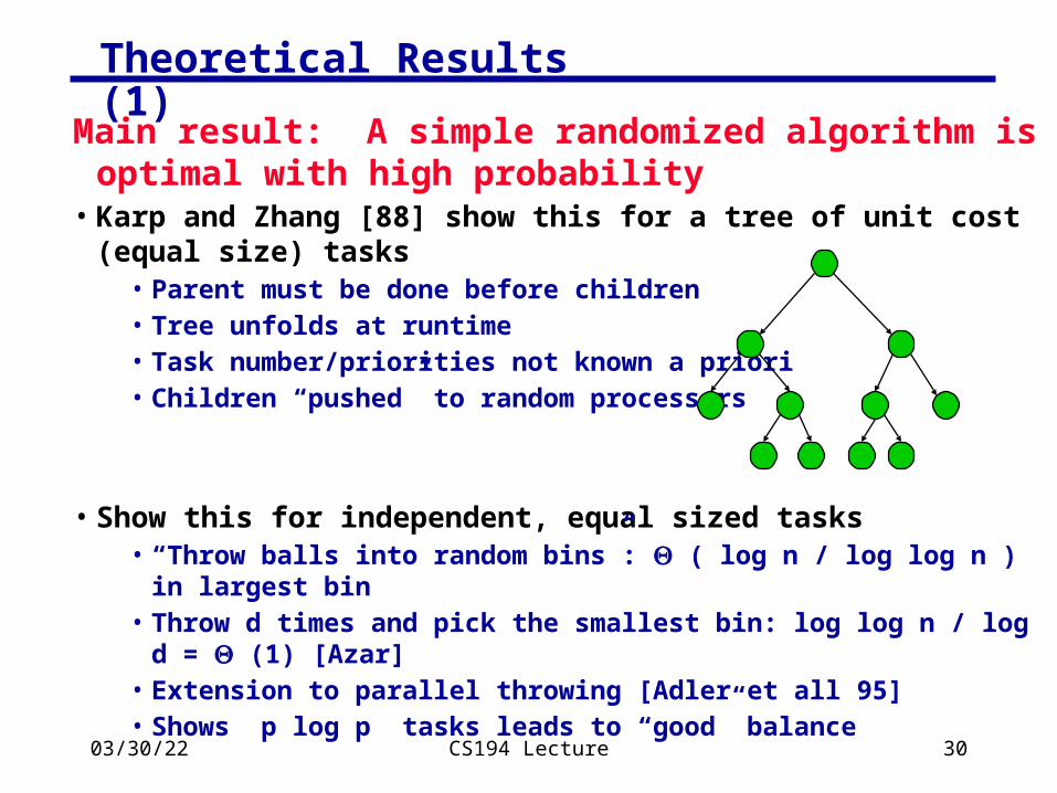
Theoretical Results (1)

Main result: A simple randomized algorithm is optimal with high probability

• Karp and Zhang [88] show this for a tree of unit cost (equal size) tasks

• Parent must be done before children• Tree unfolds at runtime• Task number/priorities not known a priori• Children “pushed” to random processors

• Show this for independent, equal sized tasks• “Throw balls into random bins”: ( log n / log log n ) in largest bin• Throw d times and pick the smallest bin: log log n / log d = (1) [Azar]• Extension to parallel throwing [Adler et all 95]• Shows p log p tasks leads to “good” balance

04/18/23 CS194 Lecture 31

Theoretical Results (2)

Main result: A simple randomized algorithm is optimal with high probability

• Blumofe and Leiserson [94] show this for a fixed task tree of variable cost tasks

• their algorithm uses task pulling (stealing) instead of pushing, which is good for locality

• I.e., when a processor becomes idle, it steals from a random processor

• also have bounds on the total memory required

• Chakrabarti et al [94] show this for a dynamic tree of variable cost tasks

• uses randomized pushing of tasks instead of pulling: worse for locality, but faster balancing in practice

• works for branch and bound, i.e. tree structure can depend on execution order

04/18/23 CS194 Lecture 32

Distributed Task Queue References

• Introduction to Parallel Computing by Kumar et al (text)• Multipol library (See C.-P. Wen, UCB PhD, 1996.)

• Part of Multipol (www.cs.berkeley.edu/projects/multipol)• Try to push tasks with high ratio of cost to compute/cost to push

• Ex: for matmul, ratio = 2n3 cost(flop) / 2n2 cost(send a word)

• Goldstein, Rogers, Grunwald, and others (independent work) have all shown

• advantages of integrating into the language framework• very lightweight thread creation

• CILK (Leiserson et al) (supertech.lcs.mit.edu/cilk)• Space bound on task stealing

• X10 from IBM

04/18/23 CS194 Lecture 33

Diffusion-Based Load Balancing

• In the randomized schemes, the machine is treated as fully-connected.

• Diffusion-based load balancing takes topology into account

• Locality properties better than prior work• Load balancing somewhat slower than randomized• Cost of tasks must be known at creation time• No dependencies between tasks

04/18/23 CS194 Lecture 34

Diffusion-based load balancing

• The machine is modeled as a graph• At each step, we compute the weight of task

remaining on each processor• This is simply the number if they are unit cost tasks

• Each processor compares its weight with its neighbors and performs some averaging

• Analysis using Markov chains

• See Ghosh et al, SPAA96 for a second order diffusive load balancing algorithm

• takes into account amount of work sent last time• avoids some oscillation of first order schemes

• Note: locality is still not a major concern, although balancing with neighbors may be better than random

04/18/23 CS194 Lecture 35

Load Balancing Summary

• Techniques so far deal with• Unpredictable loads online algorithms• Two scenarios

• Fixed set of tasks with unknown costs: self-scheduling• Dynamically unfolding set of tasks: work stealing

• Little concern over locality, except• Stealing (pulling) is better than pushing (sending work away)• When you steal, steal the oldest tasks which are likely to

generate a lot of work

• What if locality is very important?• Load balancing based on data partitioning• If equal amounts of work per grid point, divide grid points evenly• This is what you’re doing in HW3• Optimize locality by minimizing surface area (perimeter in 2D)

where communication occurs; minimize aspect ratio of blocks

• What if we know the task graph structure in advance?• More algorithms for these other scenarios

04/18/23 CS194 Lecture 36

Project Discussion

04/18/23 CS194 Lecture 37

Project outline

• Select an application or algorithm (or set of algorithms) Choose something you are personally interested in that has potential to need more compute power

• Machine learning (done for GPUs in CS267)• Algorithm from “physics” game, e.g., collision detection• Sorting algorithms• Parsing html (ongoing project)• Speech or image processing algorithm• What are games, medicine, SecondLife, etc. limited by?

• Select a machine (or multiple machines)• Preferably multicore/multisocket SMP, GPU, Cell (>= 8 cores)

• Proposal (due Fri, Oct 19): Describe problem, machine, predict bottlenecks and likely parallelism (~1-page)

04/18/23 CS194 Lecture 38

Project continued

Project steps:• Implement a parallel algorithm on machine(s)• Analyze performance (!); develop performance model

• Serial work• Critical path in task graph (can’t go faster)• Memory bandwidth, arithmetic performance, etc.

• Tune performance• We will have preliminary feedback sessions in class!• Write up results with graphs, models, etc.

• Length is not important, but think of 8-10 pages

• Note: what is the question you will attempt to answer?• X machine is better than Y for this algorithm (and why)• This algorithm will scale linearly on X (for how many procs?)• This algorithm is entirely limited by memory bandwidth