Tre

6.13 Greenhouse ClimatesM Pagani, Yale University, New Haven, CT, USAM Huber, Purdue University, West Lafayette, IN, USAB Sageman, Northwestern University, Evanston, IL, USA

ã 2014 Elsevier Ltd. All rights reserved.

6.13.1 Introduction 2816.13.2 Temperatures: An Evolving Perspective 2816.13.2.1 A New Generation of Temperature Proxy Records 2826.13.3 The Paleocene–Eocene Thermal Maximum and Other Eocene Hyperthermals 2846.13.4 The Case For and Against Glaciations During Greenhouse Climates 2866.13.5 Greenhouse Climates and Organic Carbon Burial 2886.13.6 Climate Modeling and the Challenges of Greenhouse Temperature Distributions 2906.13.6.1 The Low Temperature Gradient Problem in a Warmer World 2906.13.6.2 The Role of Ocean Heat Transport 2916.13.6.3 The Role of Atmospheric Heat Transport 2916.13.6.4 The Role of Vegetation 2936.13.7 Estimates of Atmospheric Carbon Dioxide in Relationship to Greenhouse Climates 2936.13.7.1 Greenhouse CO2 and Climate Sensitivity 2946.13.8 Summary 297References 297

6.13.1 Introduction

The state of Earth’s climate, vieweddimly through bits of dirt and

bone, appears to have waxed and waned, shifted and flipped,

since the start of its long history. Celestial, tectonic, and biolog-

ical forces leave nothing untouched, perpetually pushing the

internal variability of climate this way and that, and sometimes

over the edge. A wide range of periodic and quasi-periodic

changes in physical sedimentation, biological processes, chemi-

cal reactions, and atmospheric effects, have been surmised and

detected, forced by both allochthonous and autochthonous

beats. The notion promoted by Al Fischer, of long 30–36 Ma

cycles (Dorman, 1968; Fischer and Arthur, 1977) riding on

300 Ma supercycles (Fischer and Arthur, 1977), expressed a

world responding to changes in atmospheric carbon dioxide

concentration and toggling between dominant ‘greenhouse’

and ‘icehouse’ states (Fischer, 1981, 1982; Frakes et al., 1992)

that was reflected in marine and terrestrial diversity, ocean struc-

ture, marine redox conditions, carbonate saturation, and extent

of glaciation. Long-term changes in climate were assumed driven

by carbon dioxide concentration (Chamberlin, 1899) – a view

consistent with some of the first estimates of climate sensitivity

to CO2 (Arrhenius, 1896; Plass, 1956), and one that can now be

tested as improvedmethods of quantifying ancient carbon diox-

ide concentrations.

Greenhouse climates, which lack substantial accumulations

of permanent continental ice because of temperatures much

warmer than the Holocene average, are the common condition

for the past 540 Ma. Cold, glacial conditions characteristic of our

modern Earth are unusual. But greenhouse climates are also

characterized by a pervasive variability that appears sensitive to

both internal drivers and external (i.e., orbital) variations, and

can be characterized by abrupt climate shifts, indicative of either

thresholds in the climate system, strongly nonlinear interactions,

atise on Geochemistry 2nd Edition http://dx.doi.org/10.1016/B978-0-08-095975

or sudden changes in climatic forcing factors. One of the major

objectives of climate science is to understand these dynamics and

ultimately improve our ability to predict future climate change.

The investigation of greenhouse climates is making substantial

progress toward this goal, driven by innovations in paleoenvir-

onmental reconstructions for both marine and terrestrial realms,

and by significant improvements in paleoclimate modeling.

Paleotemperature proxies, including carbonate oxygen isotopic

compositions and Mg/Ca ratios, and other methods that might

still be considered works-in-progress, such as U37K’, TEX86, and

clumped isotopes, are now complimented by new proxy

reconstructions of atmospheric CO2 that allow us to address

the long-standing challenge of constraining climate sensitivity

to greenhouse gas forcing.

For this work, we review proxy records and modeling stud-

ies for the most recent greenhouse climate state and present a

broad overview of our evolving perspectives including the

primary agents forcing global climate and the feedbacks

responsible for the observed temperature distributions.

6.13.2 Temperatures: An Evolving Perspective

In this review, greenhouse climates are considered to be inter-

vals too warm to sustain substantial continental glaciation. By

this definition, the last major greenhouse interval persisted

from the late Permian, �260 Ma ago (Montanez and Poulsen,

2013), to the Eocene/Oligocene boundary (�35 Ma ago).

Because so much more is known about the climates of the

Cretaceous and early Cenozoic from proxy records and model-

ing studies, we restrict our discussion to these intervals of time.

The Cretaceous has long been recognized for its unusual

warmth (Hallam, 1985; Urey et al., 1951). Climatic history

gleaned from some of the first oxygen isotope measurements

-7.01314-0 281

0 15 30 45 60 75 90-30

-20

-10

0

10

20

30

40

50

Tem

per

atur

e (°

C)

Absolute latitude

Cenomanian (94 Ma)

Maastrichtian (66 Ma)

Eocene (55 Ma)

Holocene

Comparison of warm period zonal temperatures

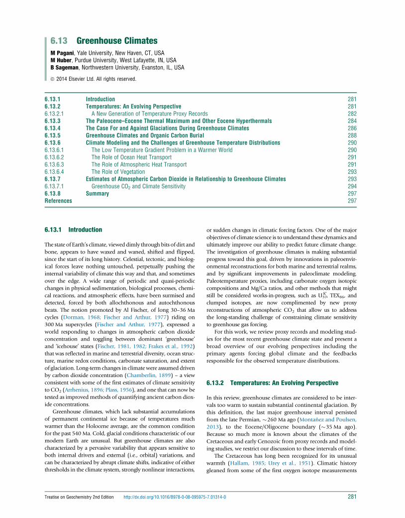
Figure 1 Zonal sea-surface temperature profiles based on d18O valuesof carbonates that were likely diagenetically altered (modified fromCrowley T and Zachos JC (2000) Comparison of zonal temperatureprofiles for past warm time periods. In: Huber BT, MacLeod KG, andWing SL (eds.)Warm Climates in Earth History, pp. 50–766. Cambridge:Cambridge University Press). Polar temperatures (black filled circles)are based on benthic foraminiferal d18O values. These temperaturesare no longer considered valid.

282 Greenhouse Climates

(d18O) of belemnites, brachiopods, inoceramids, and oysters,

show a broad multimillion-year temperature rise-and-fall from

the Albian through the Maastrichtian, with peak temperatures

near the early Campanian (Lowenstam and Epstein, 1954).

Subsequent isotope analyses of foraminifera (Douglas and

Savin, 1973, 1975; Savin, 1977; Savin et al., 1975; Shackleton

and Kennett, 1975) and bivalves (Dorman, 1966) extended the

appearance of very warm ocean temperature records through

the early Cenozoic, but with another peak in temperature

sometime during the Eocene followed by a long decline and

precipitous drops in temperature toward our modern icehouse

state. Although cautiously quantitative, these earliest isotope

measurements imply much warmer temperatures for the Cre-

taceous and Eocene, revealing a distinctly unique view of

ancient climate – a world with an expanded tropical realm

unlikely to support ‘permanent’ polar ice sheets (i.e., those

with durations in excess of millions of years).

Terrestrial temperature estimates, inferred from leaf margin

analysis and the composition of fossil floras, also imply warm

climates throughout the Cretaceous and early Eocene (Askin,

1990; Axelrod, 1984; Kowalski and Dilcher, 2002; Poole et al.,

2005; Uhl et al., 2007a,b; Wolfe, 1978, 1994). Fossil floras from

the North Slope of Alaska (Parrish and Spicer, 1988; Spicer and

Parrish, 1986) and northeastern Russia (Spicer et al., 2002)

indicate that high Arctic mean annual temperature (MAT) fell

from�13 �C in the mid-Cretaceous (Herman and Spicer, 1996;

Spicer et al., 2002) to 2–8 �C by the Maastrichtian in areas that

currently have MAT of�14 �C (Spicer et al., 2008). Warm polar

regions with winter temperatures above freezing are also

inferred from the occurrence of fossil crocodilians and other

aquatic vertebrates at mid- to high latitudes during the Creta-

ceous (Markwick, 1998, 2007; Tarduno et al., 1998). The recent

discovery of Late Cretaceous frost-intolerant floras in the remote

interior of Siberia far from ameliorating effects of the ocean,

allows a MAT reconstruction of�12 �C, which is 10 �C warmer

than model simulations (Spicer et al., 2008).

Oxygen isotope compositions of carbonates have been

broadly applied to constrain MAT and meridional-temperature

gradients. From the start, the role of diagenetic alteration and

selective preservation in producing anomalously cool tropical

temperatures was a leading issue in the minds of researchers

(Savin et al., 1975). But even corrections for temperature biases

resulting from diagenetic alteration resulted in the appearance

of relatively cool tropical SSTs (i.e., tropical temperatures sim-

ilar to or colder than today with much warmer temperatures

poleward) during the Cretaceous (Barron, 1983; Crowley and

Zachos, 2000) (Figure 1).

The earliest attempts to model Cretaceous temperatures

resulted in a poor fit with proxy data and suggested that cool

tropical SSTs inferred from oxygen isotopes needed to be re-

evaluated (Barron et al., 1981; Crowley and Zachos, 2000;

Poulsen et al., 1999; Saltzman and Barron, 1982). Suspicions

of spurious temperature estimates (Savin et al., 1975) were

largely ignored, and the resulting combination of a cool tropical

realm (as much as 6.5 �C cooler than today; D’Hondt and

Arthur, 1996) occurring with extraordinarily warm high lati-

tudes (D’Hondt and Arthur, 1996; Huber et al., 1995;

Sellwood et al., 1994) spawned novel modeling exercises to

explain the apparent phenomena. This led some to conclude

that the climate system alters its meridional-temperature

gradient in such a way as to minimize global mean-temperature

change and implied a very small or even zero climate sensitivity

to forcing (Lindzen, 1993, 1994, 1997; Lindzen and Farrell,

1977; Sun and Lindzen, 1993). However, we now recognize

that many of the cool tropical temperature estimates derived

from oxygen isotope measurements of Cretaceous and Eocene

fossils reflect diagenetic cements and recrystallization that pro-

mote cooler temperature estimates, particularly for warm trop-

ical surface-waters (Figure 1), to far greater extent than initially

assumed (Bice et al., 2006; Head et al., 2009; Huber, 2009;

Huber and Sloan, 2000; Norris et al., 2002; Pearson et al.,

2001; Schrag, 1999). It is now well accepted that tropical green-

house temperatures were warmer than modern values, but the

degree to which previous reconstructions were cold-biased has

only been fully appreciated in the past decade.

6.13.2.1 A New Generation of Temperature Proxy Records

Isotopic and elemental ratio evidence for substantial low-

latitude warming during the most recent greenhouse interval

is increasingly apparent (Bice et al., 2003, 2006; Huber, 1998;

Norris and Wilson, 1998). Temperature estimates from d18Oand Mg/Ca values of extremely well-preserved surface-dwelling

foraminifera have raised tropical to subtropical temperatures

for the middle- (Bornemann et al., 2008; Clarke and Jenkyns,

1999; Norris and Wilson, 1998; Norris et al., 2002; Wilson and

Norris, 2001; Wilson et al., 2002) to late Cretaceous (Pearson

et al., 2001; Wilson and Opdyke, 1996) and early-to-middle

Eocene (Pearson et al., 2001, 2007; Sexton et al., 2006; Tripati

et al., 2003) to 30–37 �C – significantly higher than modern,

but large uncertainties in absolute values remain (Huber,

2008). For example, foraminiferal oxygen isotopic composi-

tions are affected by ocean pH and its influence on the propor-

tion of HCO3�/CO3

2�, and ultimately, the thermodynamic

661 0 −1 −2 −3 −4

Temperature (˚C)

68

7072747678

80828486889092949698

100102104106108110112114

8 12 16 20 24 28 32A

ge (M

a)

δ18OBenthic

(‰, PDB)

E. Maastrichtiancooling/glaciation?

Maa

st.

Cam

pan

ian

Mid

-Cre

tace

ous

clim

ate

max

imum

San

Con

.Tu

ron.

Cen

oman

.A

lbia

nA

pt.

OAE 1b

OAE 1d

OAE 2

Glaciation?

OAE 3?

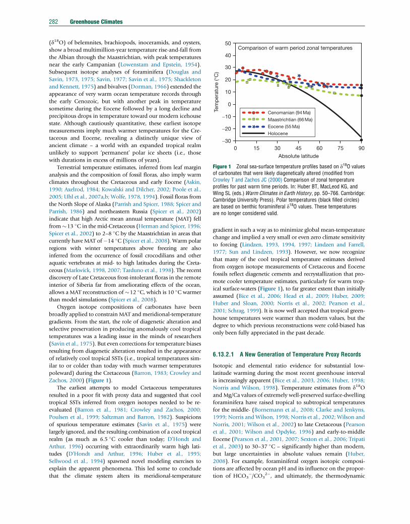
Figure 2 Stable oxygen isotope compilation of Cretaceous benthicforaminifera (modified from Friedrich O, Norris RD, and Erbacher J(2012) Evolution of middle to Late Cretaceous oceans – A 55 m.y. recordof Earth’s temperature and carbon cycle. Geology 40: 107–110). Blacksymbols represent North Atlantic Ocean, gray symbols; southern highlatitudes, red symbols; Pacific Ocean, blue symbols; subtropical SouthAtlantic Ocean, green symbols; Indian Ocean. OAE, oceanic anoxic event.Some of the data derive from exceptionally well-preserved (glassy)foraminiferal tests from the western equatorial Atlantic at Demerara Rise(Friedrich et al., 2012).

Greenhouse Climates 283

distribution of oxygen isotopes among carbonate species

(Spero et al., 1997; Zeebe, 1999). Higher CO2 concentrations

and subsequently lower seawater pH leads to a greater isotopic

fractionation between water and carbonate (Zeebe, 1999). As a

result, if atmospheric CO2 concentrations are roughly as high

as geochemical models predict (3–8 times modern values with

resulting seawater pH values of 7.9–7.7), it is likely that even

the best-preserved Cretaceous carbonates express minimum

estimates, with an excess of 2–3.5 �C hidden in isotope effects

(Zeebe, 2001). Further, accurate temperature and gradient

assessments require knowledge of the oxygen isotopic composi-

tion of shallow seawater (d18Osw) on the regional scale, given

the importance of spatial variability in precipitation and evapo-

ration, potential riverine inputs, and watermass transport by the

ocean circulation. Simulations of d18Osw during greenhouse

conditions suggest significant and differential errors in zonal

temperature reconstructions if not properly taken into account

(Poulsen et al., 1999; Roberts et al., 2009; Roche et al., 2006;

Tindall et al., 2010; Zachos et al., 1994; Zhou et al., 2008).

The advent of the new organic temperature proxy TEX86 has

also pushed SST estimates higher. The TEX86 proxy is founded

on the distribution of the membrane lipids of marine

Thaumarchaeota – isoprenoid glycerol dibiphytanyl glycerol

tetraethers (i.e., GDGTs) (Schouten et al., 2002). Ratios of

GDGTs that vary in the number of cyclopentane moieties

have been calibrated to sea-surface temperatures in the modern

ocean with an uncertainty of as much as ��4 �C (Kim et al.,

2008, 2010; Liu et al., 2009; Schouten et al., 2002, 2003).

TEX86 data suggest early- (Dumitresc et al., 2006; Jenkyns

et al., 2012; Littler et al., 2011) to middle Cretaceous tropical

conditions (Forster et al., 2007a,b; Schouten et al., 2003) of

32–36 �C to over 45 �C depending on which version of the

TEX86 temperature calibration (Kim et al., 2010) is applied.

Mid- to high-latitude temperatures during the early (Littler

et al., 2011) and late Cretaceous (Jenkyns et al., 2004) also

appear much warmer viewed through this proxy lens.

The accumulated data support an evolution of temperature

from a cooler (although still warm compared to modern) early

Cretaceous to peak warming by the Turonian (�90–94 Ma) and

returning to cooler temperatures by latest Cretaceous (Barrera

et al., 1987; Davies et al., 2009; Friedrich et al., 2012; Pirrie and

Marshall, 1990; Wilf, 2000) and early Paleocene (Wilf, 2000;

Zachos et al., 2001) (Figure 2). Cooler conditions gave way to a

trend of rising global temperatures that eventually peaked in the

early Eocene (Cramer et al., 2009). Carbonate isotope records

(Friedrich et al., 2012; Hollis et al., 2009; Zachos et al., 2001,

2006), distribution of vegetation (Basinger et al., 1994;

Greenwood and Wing, 1995; Wilf et al., 2003), and reptile

fossils (Eberle and Greenwood, 2012; Estes and Hutchison,

1980; Hutchinson, 1982; Markwick, 2007), as well as recent

TEX86 values (Brinkhuis et al., 2006; Creech et al., 2010; Hollis

et al., 2009; Sluijs et al., 2006; Zachos et al., 2006) indicate a

very warm early Eocene (55–48 Ma), particularly at high lati-

tudes, although probably cooler than the extraordinary warmth

of the middle Cretaceous (Friedrich et al., 2012).

Continental annual-mean and winter temperatures during

the early Eocene were clearly warmer than modern conditions,

with greatly reduced meridional-temperature gradients

(Greenwood andWing, 1995; Wolfe, 1994). At times, crocodiles

(Hutchinson, 1982), tapir-likemammals (Eberle, 2005), andpalm

trees (Sluijs et al., 2009) flourished around the Arctic Ocean with

warm, sometimes brackish surface waters (Brinkhuis et al., 2006;

Speelman et al., 2009). Ocean bottom-water temperatures,

inferred from oxygen isotope or Mg/Ca compositions of

benthic foraminifera were �10–12 �C higher than modern

values (Cramer et al., 2009; Lear et al., 2000; Miller et al.,

1987; Zachos et al., 1994), implying that deep-water source

regions experienced winter temperatures well above freezing.

Recent palynological results from Antarctica during peak

warming of the Eocene show thermophyllic flora with contain-

ing palms and Bombacoideae – clear evidence that winter

temperatures were well above freezing (Pross et al., 2012).

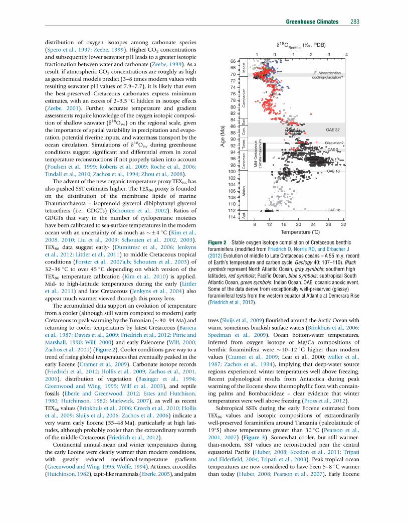
Subtropical SSTs during the early Eocene estimated from

TEX86 values and isotopic compositions of extraordinarily

well-preserved foraminifera around Tanzania (paleolatitude of

19�S) show temperatures greater than 30 �C (Pearson et al.,

2001, 2007) (Figure 3). Somewhat cooler, but still warmer-

than-modern, SST values are reconstructed near the central

equatorial Pacific (Huber, 2008; Kozdon et al., 2011; Tripati

and Elderfield, 2004; Tripati et al., 2003). Peak tropical ocean

temperatures are now considered to have been 5–8 �C warmer

than today (Huber, 2008; Pearson et al., 2007). Early Eocene

Age

(Ma)

0

5

10

15

20

25

30

35

40

45

50

55

60

65

70

75

80

85

90

95

100

105

110

115

02 4 -2 -4

δ18O (‰, PDB)

OAE 1b

OAE 2

K/T

PETM

Oi-1

Mi-1

A.

Alb

ian

Cen

. Tu.

Co

SC

amp

an.

Ma.

Pal

eoc.

Eoc

ene

Olig

.M

ioce

neP

I.

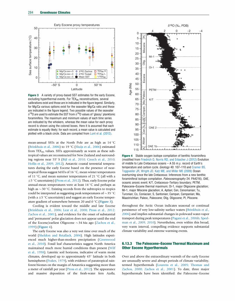
Figure 4 Stable oxygen isotope compilation of benthic foraminifera(modified from Friedrich O, Norris RD, and Erbacher J (2012) Evolutionof middle to Late Cretaceous oceans – A 55 m.y. record of Earth’stemperature and carbon cycle. Geology 40: 107–110 and Cramer BS,Toggweiler JR, Wright JD, Katz ME, and Miller ME (2009) Oceanoverturning since the late Cretaceous: Inferences from a new benthicforaminiferal isotope compilation. Paleoceanography 24: PA4216). OAE,oceanic anoxic event; K/T, Cretaceous–Tertiary boundary; PETM,Paleocene–Eocene thermal maximum; Oi-1, major Oligocene glaciation;Mi-1, major Miocene glaciation; A, Aptian; Cen, Cenomanian; Tu,Turonian; Co, Coniacian; S, Santonian; Campan, Campanian; Ma,Maastrichtian; Paleoc, Paleocene; Olig, Oligocene; Pl, Pliocene.

Early Eocene proxy temperatures

−50� S 0 50� NLatitude

0

10

20

30

40

50S

ea s

urfa

ce t

emp

erat

ure

(°C

)

Mean SST

Mg/Ca sw = 3Mg/Ca sw = 4Mg/Ca sw = 5

δ18O Zachosδ18O Tindall

TEX86 HTEX86 L1/TEX86

Figure 3 A variety of proxy-based SST estimates for the early Eocene,excluding hyperthermal events. For TEX86 reconstructions, severalcalibrations exist and those are in indicated in the figure legend. Similarly,for Mg/Ca various options exist for the seawater Mg/Ca ratio and thoseare indicated in the figure legend. Two possible values of the seawaterd18O are used to estimate the SST from d18O values of ’glassy’ planktonicforaminifera. The maximum and minimum values of each time seriesare indicated by the whiskers, whereas the mean value for each proxyrecord is shown using the colored boxes. Here it is assumed that eachestimate is equally likely; for each record, a mean value is calculated andplotted with a black circle. Data are compiled from Lunt et al. (2012).

284 Greenhouse Climates

mean-annual SSTs at the North Pole are as high as 14 �C(Brinkhuis et al., 2006) to 19 �C (Sluijs et al., 2006) estimated

from TEX86 values. SSTs approximately as warm as these sub-

tropical values are reconstructed for New Zealand and surround-

ing regions near 55� S (Bijl et al., 2010; Creech et al., 2010;

Hollis et al., 2009, 2012). Antarctic coastal terrestrial tempera-

tures during the early Eocene based on the presence of near-

tropical floras suggest MATs of 16 �C, mean winter temperatures

of 11 �C, and mean summer temperatures of 21 �C (all with a

�5 �C uncertainty) (Pross et al., 2012). Thus, early Eocene polar

annual-mean temperatures were at least 14 �C and perhaps as

high as �30 �C. Existing records from the subtropics to tropics

could be interpreted as suggesting peak temperatures of�35 �C(with a �5 �C uncertainty) and suggest an early Eocene temper-

ature gradient of somewhere between 20 and 0 �C (Figure 3).

Cooling is evident toward the middle and late Eocene

(Brinkhuis et al., 2006; Lear et al., 2008; Pross et al., 2012;

Zachos et al., 2001), and evidence for the onset of substantial

and ‘permanent’ polar glaciation does not appear until the end

of the Eocene/earliest Oligocene �34 Ma ago (Zachos et al.,

1999) (Figure 4).

The early Eocene was also a very wet time over much of the

world (Sheldon and Retallack, 2004). High latitudes experi-

enced much higher-than-modern precipitation (Greenwood

et al., 2010). Fossil leaf characteristics suggest North America

maintained much more humid conditions than present (Wilf

et al., 1998). Lateritic soil horizons, indicative of warm moist

climates, developed up to approximately 45� latitude in both

hemispheres (Frakes, 1979), with evidence of paratropical rain-

forest biomes on the margin of Antarctica suggesting more than

a meter of rainfall per year (Pross et al., 2012). The appearance

and massive deposition of the fresh-water fern Azolla,

throughout the Arctic Ocean indicates seasonal or continual

persistence of very low-salinity surface waters (Brinkhuis et al.,

2006) and implies substantial changes in poleward water-vapor

transport during peak temperatures (Pagani et al., 2006b; Speel-

man et al., 2009, 2010). Nevertheless, even within this broad,

very warm interval, compelling evidence supports substantial

climate variability and extreme warming events.

6.13.3 The Paleocene–Eocene Thermal Maximum andOther Eocene Hyperthermals

Over and above the extraordinary warmth of the early Eocene

are unusually severe and abrupt periods of climate variability,

termed hyperthermals (Lourens et al., 2005; Thomas and

Zachos, 2000; Zachos et al., 2001). To date, three major

hyperthermals have been identified: the Paleocene–Eocene

I2 I1H2

ETM2ETM3

ETM

1

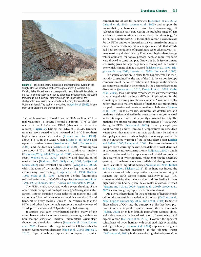
Figure 5 The sedimentary expression of hyperthermal events in theScaglia Rossa Formation of the Possagno outcrop (Southern Alps,Veneto, Italy). Hyperthermals correspond to marly interval intercalated inthe red limestone succession due to carbonate dissolution and increasedterrigenous input. Cyclical marly layers in the upper part of thestratigraphic succession corresponds to the Early Eocene ClimaticOptimum interval. The section is described in Agnini et al. (2006). Imagefrom Luca Giusberti and Domenico Rio.

Greenhouse Climates 285

Thermal Maximum (referred to as the PETM or Eocene Ther-

mal Maximum 1), Eocene Thermal Maximum (ETM) 2 (also

referred to as ELMO), and ETM3 (also referred to as the

X-event) (Figure 5). During the PETM at �55 Ma, tempera-

tures are reconstructed to have increased by 5–8 �C in southern

high-latitude sea-surface waters (Kennett and Stott, 1990),

about 4–5 �C in the Arctic Ocean (Sluijs et al., 2006) and

equatorial surface waters (Kozdon et al., 2011; Zachos et al.,

2005), and the deep sea (Zachos et al., 2001). Warming was

also about 5 �C at middle latitudes in continental interiors

(Fricke andWing, 2004; Wing et al., 2005) and along the Arctic

coast (Weijers et al., 2007). Diversity and distribution of

marine biota (Bralower, 2002; Kelly et al., 2001; Speijer and

Morsi, 2002) and terrestrial flora shifted (Wing et al., 2005),

with migration of thermophilic biota to high latitudes and

evolutionary turnover (e.g., Gingerich et al., 1980; Hooker,

1996; Maas et al., 1995). Deep-sea benthic foraminifera

suffered extinction of 30–50% of species (Kennett and Stott,

1991, 1995; Thomas, 2007; Thomas and Shackleton, 1996).

The PETM is also associated with a severe shoaling of the

ocean calcite compensation depth and a�3.0% negative stable

carbon isotope excursion (CIE) reflected in marine and soil

carbonates. The confluence of ocean acidification, the CIE, and

temperature proxy records, leads to the conclusion that the

PETM and other hyperthermals represent a massive release of13C-depleted carbon and CO2-induced global warming.

It appears that each hyperthermal exhibits many of the

same characteristics including a transient warming, a stable car-

bon isotope excursion, benthic foraminiferal assemblage

changes, and dissolution horizons (Lourens et al., 2005; Zachos

et al., 2005). However, the magnitude of the CIE for each sub-

sequent warming event decreases (Sluijs et al., 2009; Stap et al.,

2010). Hyperthermals also appear to correspond to similar

combinations of orbital parameters (DeConto et al., 2012;

Galeotti et al., 2010; Lourens et al., 2005) and support the

notion that hyperthermals were driven by a common trigger. If

Paleocene climate sensitivity was in the probable range of ‘fast

feedback’ climate sensitivities for modern conditions (e.g., 2–

4.5 �C per doubling of CO2), the implied carbon dioxide release

for the PETM and other hyperthermals was massive in order to

cause the observed temperature changes in a world that already

had high concentrations of greenhouse gases. Alternatively, cli-

mate sensitivity during the early Eocene was higher than average

values estimated for today, perhaps because more feedbacks

were allowed to come into play (known as Earth System climate

sensitivity) given the largemagnitude of forcing and the duration

over which climate change occurred (Dickens et al., 1995; Hig-

gins and Schrag, 2006; Pagani et al., 2006b; Zeebe et al., 2009).

The source of carbon to cause these hyperthermals is theo-

retically constrained by the size of the CIE, the carbon isotope

composition of the source carbon, and changes in the carbon-

ate compensation depth determined by the degree of carbonate

dissolution (Jones et al., 2010; Panchuk et al., 2008; Zeebe

et al., 2009). Two dominant hypotheses for extreme warming

have emerged with distinctly different implications for the

climate system during greenhouse climates. A common expla-

nation invokes a massive release of methane gas precariously

trapped in marine sediments as methane clathrates (Dickens

et al., 1995). In this scenario, clathrates are destabilized and

methane is either oxidized in the water column and/or released

to the atmosphere where it is quickly converted to CO2. The

methane hypothesis requires the initial release of �3000 PgC

during the PETM (Zeebe et al., 2009) driven by a rapid pre-

event warming and/or threshold temperatures in very deep

waters given that methane clathrates would only be stable in

deep pelagic sediments where high sedimentary pressures off-

set the enhanced warmth of the Eocene deep ocean (Archer

and Buffett, 2005; Archer et al., 2004). The cause and nature of

this ‘pre-event warming’ has not been defined or well identified

in paleotemperature reconstructions (Sluijs et al., 2007), and is

further constrained by the appearance of orbital controls on

the occurrence of hyperthermals. Whether or not the necessary

quantity of methane was even available during greenhouse

times is another important debate (Archer et al., 2004; Buffett

and Archer, 2004; Dickens, 2011). If methane was indeed the

primary source of carbon responsible for extreme warming, it

suggests that Earth System climate sensitivity to CO2 (i.e.,

climate sensitivity that includes slow and fast feedbacks) was

high during the Eocene given the estimates of carbon released

(Higgins and Schrag, 2006; Pagani et al., 2006b; Zeebe et al.,

2009), even though cryospheric effects were absent.

An alternate hypothesis for the appearance of hyperthermals

calls on the irreversible degradation of biomass (DeConto et al.,

2012; Higgins and Schrag, 2006; Kurtz et al., 2003) leading to

direct release of CO2 into the atmosphere. This has been pro-

posed to occur as tropical ecosystems crossed thermal thresholds

(Huber, 2008) or as high-latitude permafrosts warmed, dried,

and subsequently experienced oxidation of accumulated soil

organic carbon (DeConto et al., 2012). However, the apparent

coincidence of hyperthermals with combined high eccentricity

and high obliquity (Lourens et al., 2005) implicates changes in

high-latitude seasonal insolation as the ultimate trigger

(DeConto et al., 2012). In this scenario, high-latitude permafrost

286 Greenhouse Climates

catastrophically melted when the region crossed a critical tem-

perature threshold due to the combination of slow, CO2-induced

warming andwarmorbital geometries. CO2 is then released from

the oxidization of permafrost organic carbon. The upper range of

model-derived estimates for the amount of available permafrost

carbon (DeConto et al., 2012), as well as modern rates of per-

mafrost carbon sequestration and release (Schuur et al., 2008,

2009), accommodate geochemical requirements dictated by car-

bon cycle modeling (Cui et al., 2011; Panchuk et al., 2008) and

lead to much higher CO2 input and lower estimates of Earth

System climate sensitivity (Jones et al., 2010; Pagani et al.,

2006b). However, the requirement that permafrost existed on

Antarctica during the early Eocene might be hard to reconcile

with recent evidence for pervasive Antarctic coastal warmth dur-

ing the interval (Hollis et al., 2012; Pross et al., 2012).

Presently, carbon cycle models do not allow us to discrim-

inate between various carbon cycle perturbation hypotheses. In

lieu of novel results from new geochemical proxies, determin-

ing which of these hypotheses represent the primary hyperther-

mal trigger will depend on an improved understanding of how

ocean pH changed and impacted the global CCD, as well as a

clearer understanding of the limits of methane and terrestrial

carbon reservoir magnitudes and accumulation rates during a

much warmer world. Nonetheless, these hypotheses suggest

that extreme climate variability is an aspect of greenhouse

climates particularly as the climate system evolves from the

colder spectrum of the greenhouse world toward the warmest

extremes and threshold conditions.

6.13.4 The Case For and Against GlaciationsDuring Greenhouse Climates

In spite of profound global and high-latitude warmth during the

most recent greenhouse episode, arguments persist for icehouse

conditions or punctuated glaciations during the Cretaceous

(Bornemann et al., 2008; Miller, 2009; Price and Nunn, 2010;

Steuber et al., 2005) and the Eocene (Spielhagen and Tripati,

2009), challenging the notion of a strictly ice-free planet during

prevalent greenhouse conditions (Frakes and Francis, 1988).

Intriguing evidence for seasonally freezing temperatures and/or

permanent polar ice includes ice-rafted debris and lonestone-

bearing mudstones together with glendonite pseudomorphs on

Australia during the early Cretaceous Valanginian through the

Albian stages (Alley and Frakes, 2003; Frakes et al., 1995; Price,

1999; Price and Nunn, 2010). Deposits with glendonites, single

erratics, and conglomeratic clasts have also been found in

Paleocene–Eocene sections on Svalbard (Spielhagen and Tripati,

2009). Of these deposits, a distinct 2-m thick Cretaceous diamic-

tite on Flinders Range of Australia represents evidence for glacial

erosion (Alley and Frakes, 2003). Although these observations

are supportive of cool, higher latitude/altitude temperatures,

they are not considered unambiguous evidence of continental

ice sheets (Bennett and Doyle, 1996; Hay, 2008). Single erratics

and clasts can often be discounted as anomalous dispersal by

kelp or storm deposits (as discussed in Markwick, 1998), but

glendonite pseudomorphs are more difficult to discount.

Three interpretations of these sedimentological records can

be made. First, the appearance of high-latitude warmth from

nearly all the other proxies is incorrect and these climates were

actually perennially cooler than most reconstructions. While

this would certainly reduce the model-data discrepancies that

have pervaded the literature, the overwhelming bulk of proxy

evidence leads us to conclude that this argument is not valid.

The second alternative is that these are records of short, ‘cold

snaps’ (Price and Nunn, 2010) probably related to orbital

configurations that enhance polar cooling. Whether this

hypothesis is valid is debatable (Jenkyns et al., 2012), but the

argument is physically plausible. A third alternative is that

records of cool high-latitude temperatures – the presence of

glendonite pseudomorphs formed after ikaite – represent fil-

ters of the seasonal variability that are especially sensitive to

winter season temperatures. For example, the presence of ikaite

tends to be interpreted as indicating subseafloor temperatures

of <4 �C (Spielhagen and Tripati, 2009) or <7 �C (Price and

Nunn, 2010), both of which are compatible with the densest

water temperatures that might occur in the winter season in the

Arctic while still being consistent with other proxy records. In

other words, the presence of cold sensitive proxies such as

pseudomorphs could simply be revealing colder winter season

temperatures (4–7 �C) preferentially recorded in the densest

waters at depth in enclosed basins.

Interpretations of sea-level variations during the Cretaceous

and Eocene present an additional challenge to the assumption

of ice-free conditions. Recent reviews by Hay (2008) and Miller

et al. (2011) provide a comprehensive summary of the green-

house glacioeustasy debate. Evidence for glaciation rests mainly

on inferred eustatic fluctuations from stratigraphic sequences

occurring at frequencies too high for tectonic drivers. Some of

these sequences are also argued to be linked to stable isotope

variability and astronomical pacing (e.g., Boulila et al., 2012;

Gale et al., 2008; Galeotti et al., 2009). Accordingly, opposition

to greenhouse glacioeustasy falls into two broad camps: those

who question eustatic reconstructions based on ancient strati-

graphic successions (e.g., Burton et al., 1987; Fjeldskaar, 1989;

Miall, 1992; Morner, 1976) and those who argue that isotopic

data do not support changes in ice volume large enough to

account for glaciation (Ando et al., 2009; Moriya et al., 2007).

Initial estimates of eustatic sea-level- and inferred ice-volume

changes from stratigraphic sequences (Haq et al., 1987; Vail

et al., 1977) failed to adequately consider the potential for

isostatic adjustments, changes in sediment load, dynamic topog-

raphy associated with the viscous flow response of the mantle

(Lambeck and Chappell, 2001; Mitrovica et al., 2011), basin

subsidence (Christie-Blick et al., 1990; Hay, 2008; Hay and

Southam, 1977), and autocyclic depositional processes such as

delta migration and progradation (e.g., Poulsen et al., 1998). As

a consequence, those sea-level estimates appear unreasonably

large, requiring volumes of ice equal to or greater than the

current Antarctic ice sheet to wax and wane during extraordi-

narily warm periods (e.g., Hay, 2008).

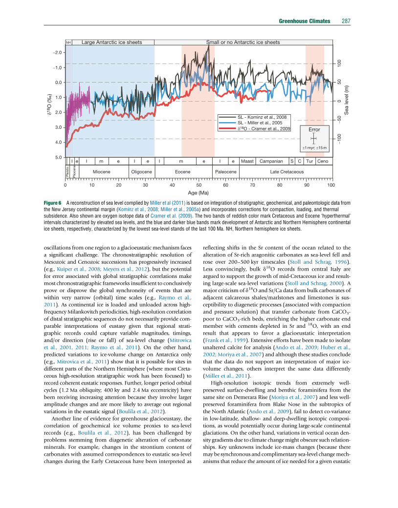
More recent sea-level reconstructions (Figure 6) that

employ corrections for isostacy, sediment loading, and subsi-

dence (e.g., Kominz et al., 2008; Miller et al., 2005a) limit

oscillations prior to the Neogene expansion of ice sheets to a

maximum of about 50 m – which would still require signifi-

cant ice volumes if glacioeustasy was the only driver. Although

there is a reasonable match between the long-term pattern in

d18O (and by inference temperature) and the long-term sea-

level record (Figure 6), the attribution of high-frequency

Error

Large Antarctic ice sheetsNH Small or no Antarctic ice sheets

SL - Kominz et al., 2008

d18O - Cramer et al., 2009

d18 O

(‰)

±1 myr; ±15 m

SL - Miller et al., 2005

Miocene

10

5.0

4.0

3.0

2.0

1.0

0.0

-1.0

-2.0

20 30 40 50 60 70 80 90 100

-100

-50

050

100

0

I I I I Ie m me e e e C

Age (Ma)

Sea

leve

l (m

)

Ple

isto

.

Plio

cene

CenoTurS

Oligocene Eocene Paleocene

CampanianMaast

Late Cretaceous

Figure 6 A reconstruction of sea level complied by Miller et al (2011) is based on integration of stratigraphic, geochemical, and paleontologic data fromthe New Jersey continental margin (Kominz et al., 2008; Miller et al., 2005a) and incorporates corrections for compaction, loading, and thermalsubsidence. Also shown are oxygen isotope data of Cramer et al. (2009). The two bands of reddish color mark Cretaceous and Eocene ‘hyperthermal’intervals characterized by elevated sea levels, and the blue and darker blue bands mark development of Antarctic and Northern Hemisphere continentalice sheets, respectively, characterized by the lowest sea-level stands of the last 100 Ma. NH, Northern hemisphere ice sheets.

Greenhouse Climates 287

oscillations from one region to a glacioeustaticmechanism faces

a significant challenge. The chronostratigraphic resolution of

Mesozoic and Cenozoic successions has progressively increased

(e.g., Kuiper et al., 2008; Meyers et al., 2012), but the potential

for error associated with global stratigraphic correlations make

most chronostratigraphic frameworks insufficient to conclusively

prove or disprove the global synchroneity of events that are

within very narrow (orbital) time scales (e.g., Raymo et al.,

2011). As continental ice is loaded and unloaded across high-

frequencyMilankovitch periodicities, high-resolution correlation

of distal stratigraphic sequences do not necessarily provide com-

parable interpretations of eustasy given that regional strati-

graphic records could capture variable magnitudes, timings,

and/or direction (rise or fall) of sea-level change (Mitrovica

et al., 2001, 2011; Raymo et al., 2011). On the other hand,

predicted variations to ice-volume change on Antarctica only

(e.g., Mitrovica et al., 2011) show that it is possible for sites in

different parts of the Northern Hemisphere (where most Creta-

ceous high-resolution stratigraphic work has been focused) to

record coherent eustatic responses. Further, longer period orbital

cycles (1.2 Ma obliquity; 400 ky and 2.4 Ma eccentricity) have

been receiving increasing attention because they involve larger

amplitude changes and are more likely to average out regional

variations in the eustatic signal (Boulila et al., 2012).

Another line of evidence for greenhouse glacioeustasy, the

correlation of geochemical ice volume proxies to sea-level

records (e.g., Boulila et al., 2012), has been challenged by

problems stemming from diagenetic alteration of carbonate

minerals. For example, changes in the strontium content of

carbonates with assumed correspondences to eustatic sea-level

changes during the Early Cretaceous have been interpreted as

reflecting shifts in the Sr content of the ocean related to the

alteration of Sr-rich aragonitic carbonates as sea-level fell and

rose over 200–500 kyr timescales (Stoll and Schrag, 1996).

Less convincingly, bulk d18O records from central Italy are

argued to support the growth of mid-Cretaceous ice and result-

ing large-scale sea-level variations (Stoll and Schrag, 2000). A

major criticism of d18O and Sr/Ca data from bulk carbonates of

adjacent calcareous shales/marlstones and limestones is sus-

ceptibility to diagenetic processes (associated with compaction

and pressure solution) that transfer carbonate from CaCO3-

poor to CaCO3-rich beds, enriching the higher carbonate end

member with cements depleted in Sr and 18O, with an end

result that appears to favor a glacioeustatic interpretation

(Frank et al., 1999). Extensive efforts have been made to isolate

unaltered calcite for analysis (Ando et al., 2009; Huber et al.,

2002; Moriya et al., 2007) and although these studies conclude

that the data do not support an interpretation of major ice-

volume changes, others interpret the same data differently

(Miller et al., 2011).

High-resolution isotopic trends from extremely well-

preserved surface-dwelling and benthic foraminifera from the

same site on Demerara Rise (Moriya et al., 2007) and less well-

preserved foraminifera from Blake Nose in the subtropics of

the North Atlantic (Ando et al., 2009), fail to detect co-variance

in low-latitude, shallow- and deep-dwelling isotopic composi-

tions, as would potentially occur during large-scale continental

glaciations. On the other hand, variations in vertical ocean den-

sity gradients due to climate changemight obscure such relation-

ships. Key unknowns include ice-mass changes (because there

may be synchronous and complimentary sea-level changemech-

anisms that reduce the amount of ice needed for a given eustatic

288 Greenhouse Climates

oscillation, and thus smaller isotopic effects), as well as assump-

tions about the isotopic composition of Cretaceous ocean water

and precipitation, which influence the proxy relationship.

The most convincing records of large magnitude sea-level

changes are high-frequency, inferred eustatic oscillations

observed during the Early- to Late Cretaceous, including some

during the peak warming of the Middle Cretaceous from the

Western Interior North America (Gale et al., 2008; Koch and

Brenner, 2009), Europe, India (Gale et al., 2002), and central

Italy (Galeotti et al., 2010, Weissert and Lini, 1991). Putatively,

eustatic sea-level estimates from New Jersey, USA and the

Russian platform for the Late Cretaceous to early Eocene

(including some for the Middle Cretaceous), which are assumed

correlative with positive changes in low-resolution benthic d18Ovalues from other locations (Huber et al., 1999, 2002), are

interpreted as �25 m of sea-level change occurring in less than

1 Ma (Miller et al., 2005a,b; Sickel et al., 2004).

Other perspectives that support the notion of greenhouse

glaciation apply TEX86 temperatures in conjunction with well-

preserved foraminiferal oxygen isotopes from the Demerara

Rise in the eastern equatorial Atlantic (Bornemann et al.,

2008; Forster et al., 2007a,b). Large changes in ice volume –

from �45 to 150% the size of the modern Antarctic ice sheet –

are calculated during peak temperatures in the Turonian on the

basis of positive d18O shifts that are unmatched by TEX86

changes. Even though the baseline tropical temperatures esti-

mated by the same study are �10 �C warmer than today (i.e.,

34–37 �C) (Bornemann et al., 2008), the authors settle on ice

volumes perhaps 60% the size of the modern Antarctic ice

sheet, given other constraints from stratigraphically inferred

sea-level changes. However, how ice sheets of this magnitude

can move on and off under apparent ‘supergreenhouse’ condi-

tions with less than 2 �C of tropical temperature change (as

indicated by TEX86 temperatures) is not addressed.

The accuracy of TEX86 temperatures is a subject of increasing

debate. Much of the current discussion is focused on the depth

of production and the ocean temperatures that the TEX86 proxy

actually reflects (e.g., Ingalls et al., 2006; Liu et al., 2009; Shah

et al., 2008). Given the potential of ammonia oxidation by

nonthermophilic Thaumarchaeota (e.g., Nicol and Schleper,

2006), depth of production over time and space can be uncon-

strained, and so the interpretation that TEX86 exclusively

reflects SST is not necessarily warranted. It also remains to be

seen if TEX86 values are solely recording temperature. For exam-

ple, other organic-based temperature proxies, such as U37K’

values and alkenone abundances are affected by species com-

position (Conte et al., 1998), salinity (Blanz et al., 2005), and

levels of nutrients and irradiance (Prahl et al., 2003). Turich

et al. (2007) challenges a strict SST interpretation for TEX86 and

argues that nutrient distributions and ecology of Archaea play

roles in the distribution of membrane lipids and the expression

of residual temperature offsets between proxy estimates and

modern observations. To date, there is no overwhelming chal-

lenge to the accuracy of TEX86 SST temperatures other than the

persistence of multiple calibrations that result in a broad range

of temperature estimates (Kim et al., 2010; Liu et al., 2009), and

the occasional observation that the estimated temperatures

reflect deeper water production rather than SST (e.g., Liu

et al., 2009). Still, a healthy concern for the accuracy of absolute

values of TEX86 temperatures, particularly across the high

latitudes during greenhouse climates is warranted given the

sometimes stark differences between TEX86 and other proxy

results (Liu et al., 2009).

If other mechanisms used to explain apparent greenhouse

eustatic oscillations, such as thermal expansion/contraction

and changes in groundwater storage in response to climate

forcing – with the potential of up to�10 m of sea-level change

(Hay, 2008) – were operative on orbital time scales, the vol-

ume of ice build-up might be modest enough to preclude large

oxygen isotopic signals (Miller, 2009). The location of signifi-

cant ice accumulation during Cretaceous and Cenozoic green-

house times is necessarily restricted to Antarctica (Hay, 2008),

and modeling studies have shown that it is possible to grow ice

sheets under conditions of elevated CO2 (DeConto and

Pollard, 2003; Flogel et al., 2011). Removal of a substantial

ice sheet, however, requires either very large increases in CO2

due to hysteresis in the Antarctic ice sheet – implying wild

swings in atmospheric CO2 concentration (Pollard and

DeConto, 2005) – or significant changes in insolation related

to linkage of long period astronomical cycles and their ampli-

fication by feedbacks such as the carbon cycle (e.g., Boulila

et al., 2012; Palike et al., 2006).

Direct evidence of Antarctic glaciation in the Cretaceous has

yet to be revealed and would provide the most unambiguous

indication of significant ice volume during extraordinary

warmth. As such, the hypothesis that greenhouse sea-level oscil-

lations were modulated by orbitally paced climatic cycles, that

also involved global ‘cold snaps’ during some of the warmest

intervals of Earth history, has yet to be conclusively

demonstrated.

6.13.5 Greenhouse Climates and OrganicCarbon Burial

The association of widespread black shale facies with green-

house climates or ‘nonglacial’ periods was recognized early on

(Chamberlin, 1906; Str�m, 1936; van der Gracht, 1931), as

was a correlation between organic matter enrichment and

distal sediment starvation during marine transgressions (e.g.,

Pettijohn, 1957). A series of papers in the 1970–1980s synthe-

sized these and other ideas into a coherent framework of

greenhouse/icehouse oscillations mediated by changes in

global volcanism, CO2 levels, surface- and deep-ocean temper-

atures, flooding of continental interiors, and changes in the

occurrence of black shale deposition (e.g., Fischer, 1982;

Fischer and Arthur, 1977). Two major greenhouse climate

intervals during the Paleozoic and Mesozoic are characterized

by widespread black shale facies, and particular attention has

been paid to the relationships between warm climates and

black shale deposition during the Devonian and Cretaceous.

Characteristics most relevant among Cretaceous black

shales are stratigraphically narrow, but widespread horizons

of exceptional organic carbon deposition that punctuate sedi-

mentary successions (e.g., Erbacher et al., 2005). These global

carbon cycle perturbations, known as ‘Oceanic Anoxic Events’

(OAEs) (Schlanger and Jenkyns, 1976) are associated with

significant positive shifts in the stable carbon isotope signature

of organic and inorganic carbon (Arthur et al., 1988; Pratt,

1985). OAEs are interpreted to reflect substantial marine

MN

PMCE

W4

W3

Scaglia Bianca

Marne a

Fucoidi

Scaglia Rossa

Maiolica

W2

W1

F

SB

SU

A

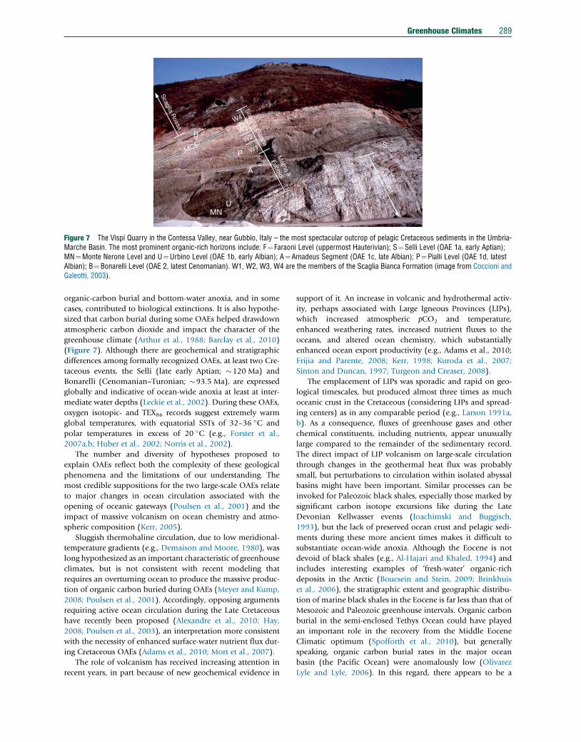
Figure 7 The Vispi Quarry in the Contessa Valley, near Gubbio, Italy – the most spectacular outcrop of pelagic Cretaceous sediments in the Umbria-Marche Basin. The most prominent organic-rich horizons include: F¼Faraoni Level (uppermost Hauterivian); S¼Selli Level (OAE 1a, early Aptian);MN¼Monte Nerone Level and U¼Urbino Level (OAE 1b, early Albian); A¼Amadeus Segment (OAE 1c, late Albian); P¼Pialli Level (OAE 1d, latestAlbian); B¼Bonarelli Level (OAE 2, latest Cenomanian). W1, W2, W3, W4 are the members of the Scaglia Bianca Formation (image from Coccioni andGaleotti, 2003).

Greenhouse Climates 289

organic-carbon burial and bottom-water anoxia, and in some

cases, contributed to biological extinctions. It is also hypothe-

sized that carbon burial during some OAEs helped drawdown

atmospheric carbon dioxide and impact the character of the

greenhouse climate (Arthur et al., 1988; Barclay et al., 2010)

(Figure 7). Although there are geochemical and stratigraphic

differences among formally recognized OAEs, at least two Cre-

taceous events, the Selli (late early Aptian; �120 Ma) and

Bonarelli (Cenomanian–Turonian; �93.5 Ma), are expressed

globally and indicative of ocean-wide anoxia at least at inter-

mediate water depths (Leckie et al., 2002). During these OAEs,

oxygen isotopic- and TEX86 records suggest extremely warm

global temperatures, with equatorial SSTs of 32–36 �C and

polar temperatures in excess of 20 �C (e.g., Forster et al.,

2007a,b; Huber et al., 2002; Norris et al., 2002).

The number and diversity of hypotheses proposed to

explain OAEs reflect both the complexity of these geological

phenomena and the limitations of our understanding. The

most credible suppositions for the two large-scale OAEs relate

to major changes in ocean circulation associated with the

opening of oceanic gateways (Poulsen et al., 2001) and the

impact of massive volcanism on ocean chemistry and atmo-

spheric composition (Kerr, 2005).

Sluggish thermohaline circulation, due to low meridional-

temperature gradients (e.g., Demaison and Moore, 1980), was

long hypothesized as an important characteristic of greenhouse

climates, but is not consistent with recent modeling that

requires an overturning ocean to produce the massive produc-

tion of organic carbon buried during OAEs (Meyer and Kump,

2008; Poulsen et al., 2001). Accordingly, opposing arguments

requiring active ocean circulation during the Late Cretaceous

have recently been proposed (Alexandre et al., 2010; Hay,

2008; Poulsen et al., 2003), an interpretation more consistent

with the necessity of enhanced surface-water nutrient flux dur-

ing Cretaceous OAEs (Adams et al., 2010; Mort et al., 2007).

The role of volcanism has received increasing attention in

recent years, in part because of new geochemical evidence in

support of it. An increase in volcanic and hydrothermal activ-

ity, perhaps associated with Large Igneous Provinces (LIPs),

which increased atmospheric pCO2 and temperature,

enhanced weathering rates, increased nutrient fluxes to the

oceans, and altered ocean chemistry, which substantially

enhanced ocean export productivity (e.g., Adams et al., 2010;

Frijia and Parente, 2008; Kerr, 1998; Kuroda et al., 2007;

Sinton and Duncan, 1997; Turgeon and Creaser, 2008).

The emplacement of LIPs was sporadic and rapid on geo-

logical timescales, but produced almost three times as much

oceanic crust in the Cretaceous (considering LIPs and spread-

ing centers) as in any comparable period (e.g., Larson 1991a,

b). As a consequence, fluxes of greenhouse gases and other

chemical constituents, including nutrients, appear unusually

large compared to the remainder of the sedimentary record.

The direct impact of LIP volcanism on large-scale circulation

through changes in the geothermal heat flux was probably

small, but perturbations to circulation within isolated abyssal

basins might have been important. Similar processes can be

invoked for Paleozoic black shales, especially those marked by

significant carbon isotope excursions like during the Late

Devonian Kellwasser events (Joachimski and Buggisch,

1993), but the lack of preserved ocean crust and pelagic sedi-

ments during these more ancient times makes it difficult to

substantiate ocean-wide anoxia. Although the Eocene is not

devoid of black shales (e.g., Al-Hajari and Khaled, 1994) and

includes interesting examples of ‘fresh-water’ organic-rich

deposits in the Arctic (Boucsein and Stein, 2009; Brinkhuis

et al., 2006), the stratigraphic extent and geographic distribu-

tion of marine black shales in the Eocene is far less than that of

Mesozoic and Paleozoic greenhouse intervals. Organic carbon

burial in the semi-enclosed Tethys Ocean could have played

an important role in the recovery from the Middle Eocene

Climatic optimum (Spofforth et al., 2010), but generally

speaking, organic carbon burial rates in the major ocean

basin (the Pacific Ocean) were anomalously low (Olivarez

Lyle and Lyle, 2006). In this regard, there appears to be a

290 Greenhouse Climates

fundamental difference between the greenhouse climates of

the Cenozoic and Mesozoic/Paleozoic, perhaps indicating

that greenhouse climates are a necessary, but not sufficient

condition for widespread black shale deposition and OAE

development. The character of OAEs demands episodic disrup-

tions and substantial nutrient fluxes to sustain the widespread

distribution of organic-rich black shales. Other mechanisms

were likely in play and major changes in ocean circulation

related to plate tectonics could have played a key role

(Robinson and Vance, 2012).

6.13.6 Climate Modeling and the Challengesof Greenhouse Temperature Distributions

Whereas modern discussions of climate change dwell in the

minutia of exceedingly short time scales and global tempera-

ture variations within tenths of a degree, greenhouse intervals

provide a means to test fundamental assumptions regarding

the first-order controls on Earth’s temperature, as well as the

strengths/weaknesses of our current climate models under

large climate changes. The primary factors driving regional

temperature distributions, and in particular, global mean tem-

perature and latitudinal temperature gradients, have been

explored through the course of climate modeling history.

Latitude90� N 60� N 30� N 0 90� S60� S30� S

50

40

30

20

10

0

Diff

eren

ce in

sur

face

tem

per

atur

e (˚C

)S

urfa

ce t

emp

erat

ure

(˚C)

40

20

0

-20

-40

-60(a)

(b)

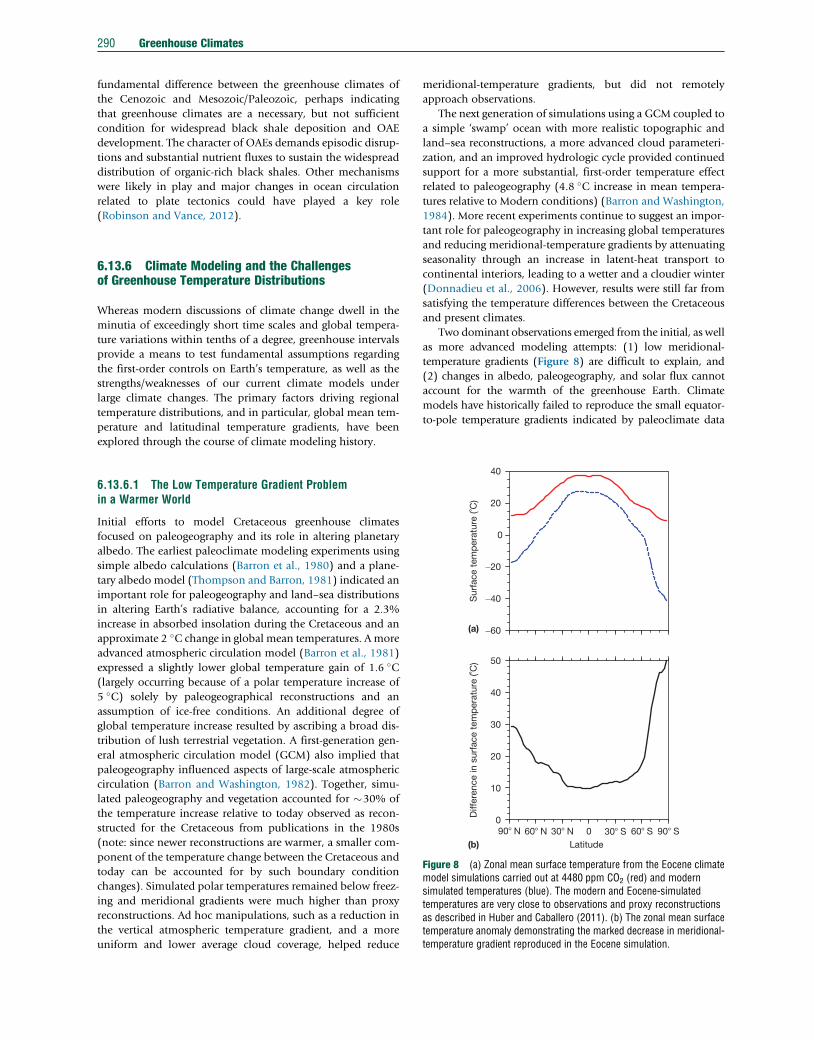
Figure 8 (a) Zonal mean surface temperature from the Eocene climatemodel simulations carried out at 4480 ppm CO2 (red) and modernsimulated temperatures (blue). The modern and Eocene-simulatedtemperatures are very close to observations and proxy reconstructionsas described in Huber and Caballero (2011). (b) The zonal mean surfacetemperature anomaly demonstrating the marked decrease in meridional-temperature gradient reproduced in the Eocene simulation.

6.13.6.1 The Low Temperature Gradient Problemin a Warmer World

Initial efforts to model Cretaceous greenhouse climates

focused on paleogeography and its role in altering planetary

albedo. The earliest paleoclimate modeling experiments using

simple albedo calculations (Barron et al., 1980) and a plane-

tary albedo model (Thompson and Barron, 1981) indicated an

important role for paleogeography and land–sea distributions

in altering Earth’s radiative balance, accounting for a 2.3%

increase in absorbed insolation during the Cretaceous and an

approximate 2 �C change in global mean temperatures. A more

advanced atmospheric circulation model (Barron et al., 1981)

expressed a slightly lower global temperature gain of 1.6 �C(largely occurring because of a polar temperature increase of

5 �C) solely by paleogeographical reconstructions and an

assumption of ice-free conditions. An additional degree of

global temperature increase resulted by ascribing a broad dis-

tribution of lush terrestrial vegetation. A first-generation gen-

eral atmospheric circulation model (GCM) also implied that

paleogeography influenced aspects of large-scale atmospheric

circulation (Barron and Washington, 1982). Together, simu-

lated paleogeography and vegetation accounted for �30% of

the temperature increase relative to today observed as recon-

structed for the Cretaceous from publications in the 1980s

(note: since newer reconstructions are warmer, a smaller com-

ponent of the temperature change between the Cretaceous and

today can be accounted for by such boundary condition

changes). Simulated polar temperatures remained below freez-

ing and meridional gradients were much higher than proxy

reconstructions. Ad hoc manipulations, such as a reduction in

the vertical atmospheric temperature gradient, and a more

uniform and lower average cloud coverage, helped reduce

meridional-temperature gradients, but did not remotely

approach observations.

The next generation of simulations using a GCM coupled to

a simple ‘swamp’ ocean with more realistic topographic and

land–sea reconstructions, a more advanced cloud parameteri-

zation, and an improved hydrologic cycle provided continued

support for a more substantial, first-order temperature effect

related to paleogeography (4.8 �C increase in mean tempera-

tures relative to Modern conditions) (Barron and Washington,

1984). More recent experiments continue to suggest an impor-

tant role for paleogeography in increasing global temperatures

and reducing meridional-temperature gradients by attenuating

seasonality through an increase in latent-heat transport to

continental interiors, leading to a wetter and a cloudier winter

(Donnadieu et al., 2006). However, results were still far from

satisfying the temperature differences between the Cretaceous

and present climates.

Two dominant observations emerged from the initial, as well

as more advanced modeling attempts: (1) low meridional-

temperature gradients (Figure 8) are difficult to explain, and

(2) changes in albedo, paleogeography, and solar flux cannot

account for the warmth of the greenhouse Earth. Climate

models have historically failed to reproduce the small equator-

to-pole temperature gradients indicated by paleoclimate data

Greenhouse Climates 291

(Barron, 1987; Deconto et al., 2000; Huber and Sloan 2000,

2001; Sloan and Rea, 1996; Valdes, 2000), a problem exacer-

bated by recent proxy temperature estimates that have raised

polar temperatures more than those in the tropics.

6.13.6.2 The Role of Ocean Heat Transport

Increased poleward heat transport by the ocean or atmosphere

has long been considered a solution to the low-gradient prob-

lem (Berry, 1922; Barron, 1987; Barron et al., 1993; Covey and

Barron, 1988; Rind and Chandler, 1991; Schmidt and Mysak,

1996). However, the supposition of low gradients propelled by

enhanced heat transport is recognized as a climate conundrum:

that is, enhanced ocean heat transport is necessary to maintain

low meridional-temperature gradients, but small meridional-

temperature gradients imply reduced density gradients,

decreased meridional overturning circulation, and hence

reduce rates of poleward heat transport. For Cretaceous and

Eocene experiments, total ocean heat transport greater than

modern values have often been necessary to avoid overly

high tropical- or cold polar temperatures (Barron et al., 1981;

Huber and Sloan, 1999). Given the physical constraints on the

atmosphere’s ability to transport more heat under equable

conditions, other mechanisms, including ocean heat transfer

in the form of low-latitude halothermal circulation, were

hypothesized. Justifications for enhanced ocean heat transport

reach back to Chamberlin (1906) who called on the produc-

tion of high-salinity waters sourced from highly evaporative,

low-latitude regions during warm periods in Earth history. But,

arguments regarding the source of deep waters and the direc-

tion of transport miss the mark (Bice andMarotzke, 2001). The

magnitude of ocean heat transport due to advective motions is

determined by the amount of cooling and the vigor of ocean

circulation. It is the heat released to the atmosphere that is

relevant and this is recorded by the cooling of watermasses as

they move poleward. Weak temperature gradients imply weak

ocean heat transport regardless of whether deep water forms at

high latitudes or low latitudes (Huber et al., 2003). Thus,

production of ‘warm saline bottom waters’ does not directly

solve the major problems of greenhouse climates.

Models that simultaneously predict the behavior of the

atmosphere and ocean have only produced total meridional

atmospheric and ocean heat transports close to modern

(Huber and Sloan, 2001; Lunt et al., 2012; Najjar et al., 2002;

Otto-Bliesner et al., 2002; Sijp et al., 2011; Winguth et al.,

2010; Zhang et al., 2011), whereas the missing heat transport

necessary to simulate greenhouse temperature gradients of

15 �C is inferred to be an extraordinary �1 Petawatt at 45�

latitude (Huber and Sloan, 1999; Huber et al., 2003) – three

times the modern value. To achieve this kind of trebling of

ocean heat transport in a world with temperature (and thus

density) gradients less than half of modern values, requires a

greater than sixfold increase in the strength of the meridional

overturning circulation. Well-established physical mechanisms

cannot provide for this kind of increase, although the idea that

vertical diffusion was much stronger in the past and that this

enhanced the ocean circulation has been explored in simple

models (Emanuel, 2002; Lyle, 1997). There is no evidence

from ocean circulation proxies for such large increases in

ocean circulation rates (Hague et al., 2012; Puceat et al.,

2007) and the associated decrease in ocean residence time it

implies, but such evidence would be very informative.

Importantly, high polar temperatures and low meridional-

temperature gradients do not necessarily imply the need for an

increase in ocean heat transport relative to modern values if

temperature gradients are at the higher end of possible values.

For example, an equator-to-pole SST difference of 24 �C (com-

pared to �50 �C today) requires near-modern heat-transport

values, whereas a gradient of 15 �C requires an ocean heat

transport three times the modern value (Huber et al., 2003).

Reconstructed polar temperatures of 25 �C in conjunction with

tropical temperatures of 31 �C would require conditions that

strongly deviate from the modern dynamical paradigm,

whereas polar temperatures of 15 �C and tropical values of

35� might not. Presently, it is impossible to definitively con-

clude whether or not we are missing a critical piece of the

puzzle in our understanding of ocean heat transport and

weak temperature gradients.

6.13.6.3 The Role of Atmospheric Heat Transport

It is often assumed that increased latent-heat transport could

account for low, meridional-temperature gradients during

greenhouse climates (e.g., Ufnar et al., 2004). However, this

conjecture is not as straightforward as it appears. Current the-

ory andmodels have shown that latent-heat transport increases

with an increasing meridional-temperature gradient for a range

of global mean temperatures – the opposite to what is required

to maintain low temperature gradients (Pierrehumbert, 2002).

But, this is complicated by nonlinearity effects introduced

by atmospheric moisture. The exponential dependence of

atmospheric saturation vapor pressure from the Clausius–

Clapeyron relation – which provides an �7% increase in

atmospheric water-vapor content per degree (�C) of global-

mean temperature increase (Held and Soden, 2006) – suggests

that during greenhouse conditions it is possible to have higher

latent-heat transport even with weaker surface temperature

gradients because there is more water vapor to transport

(Caballero and Langen, 2005; Frierson et al., 2007). The result

of Caballero and Langen (2005) show that poleward atmo-

spheric latent-heat transport increases with both increasing

temperature gradient and increasing global-mean surface tem-

perature, but global mean temperature would have to substan-

tially increase above modern conditions before this new

regime is encountered. Model predictions for latent-heat trans-

port are very sensitive to tropical temperatures because tropical

temperatures dominate the uncertainty of area-weighted global

mean temperature estimates (the region between 30�N and

30�S makes up half the Earth’s surface area). Uncertainties in

high-latitude temperatures dominate the uncertainties in a

model’s expression of the temperature gradient. Models show

that the atmosphere can transport more heat relative to mod-

ern conditions even with weaker temperature gradients, but

only if global mean temperatures are much higher than the

modern mean. Whether or not models are producing accurate

results is not currently verifiable from proxy data because

uncertainty in both tropical- and high-latitude temperatures

is large enough that the comparison produces results within

292 Greenhouse Climates

the uncertainty in the data (Huber and Caballero, 2011; Lunt

et al., 2012). What we suspect now is that most modeling work

of the past three decades was probably missing the mark in

regard to heat transport, largely because their targeted global

mean temperatures were too low and the nonlinear feedbacks

that help to decrease meridional-temperature gradients, such

as those that impact Hadley Cell width and poleward latent-

heat transport, were not accessible in older models.

If future global warming simulations are used as a guide, a

warmer world should be characterized by an intensified hydro-

logical cycle and a slightly increased Hadley Cell width, with

storm tracks displaced poleward by 2–3� latitude (Frierson

et al., 2007; Lu et al., 2007; Seager et al., 2007). But for the

Eocene and Cretaceous greenhouse, Hadley Cell width could

have shifted by 5–8� in latitude (based on the scaling of

Frierson et al. (2007)) with an associated shift in storm tracks,

and major regions of hydrological and water isotope diver-

gence. This supposition could be testable with paleoclimate

proxy data, but a subtle signal could be hard to discern with

sparsely distributed proxy data localities. However, it should be

possible to qualitatively determine an increase in the hydro-

logical cycle during greenhouse times, which would be an

important clue in explaining warm, low-gradient climates.

The characterization of ‘wet’ Eocene and Cretaceous condi-

tions is readily interpreted as reflecting an enhanced hydrolog-

ical cycle in a wetter world (Bowen et al., 2004; Greenwood

et al., 2010; Wilf et al., 1998). However, a ‘more intense’ hydro-

logical cycle refers to increased meridional water-vapor trans-

port from low- to high latitudes. Assuming steady-state

conditions, this requires an intensification of evaporation in

‘zones of net-evaporation’ and a counterbalancing increase in

precipitation in ‘zones of net-precipitation.’ This leads to an

increased meridional gradient of evaporation over precipita-

tion (Allen and Ingram, 2002; Held and Soden, 2006), consis-

tent with climate simulations of future warming that show a

general drying of the subtropics (and moistening of the deep

tropics and high latitudes). The first-order effect in the net-

surface fresh-water flux during global warming is a simple

amplification without a change in the spatial pattern. Under

steady-state conditions, there must be excess precipitation aver-

aged over the extratropics provided that evaporation exceeds

precipitation equatorward of the subtropical margins (and the

work of Ziegler et al., 2003 suggests that this has been the case

since the Permian). Thus, drying (or salinification) of the sub-

tropical regions is consistent with an increase in the strength of

the hydrological cycle with a compensating moistening in high

latitudes. In other words, during times with a more intense

hydrological system, some regionsmust get drier ormore saline

(in addition to the enhanced effectivemoisture in extra-tropical

regions normally noted in paleoclimate proxy studies) to sup-

port increased hydrological cycles and latent-heat transport

elsewhere. This pattern appears to be playing itself out in mod-

ern hydrological records (Zhang et al., 2007), and some evi-

dence indicates that a similar result occurred during Eocene

hyperthermals (Pagani et al., 2006a), but conclusions are not

firm, in large part because adequate records showing subtrop-

ical drying or salinification have not be found.

Sediments recovered from the central Arctic Ocean provided

the first opportunity to directly evaluate the environmental

response at the North Pole during intense warming (Moran

et al., 2006). Stable hydrogen (dD) and carbon (d13C) isotopemeasurements of waxes derived from terrestrial- and aquatic

plants show substantial changes in hydrology, including surface

water salinity and precipitation, and suggest that Arctic PETM

precipitation was D-enriched relative to today, with hydrogen

isotopic compositions comparable with modern, mid-latitude

precipitation (Pagani et al., 2006a).

D-enriched Arctic precipitation during the PETM could have

resulted from two possible end-member processes, including

changes in proximal evaporative sources or a decrease in large-

scale (hemispheric to global) meridional (or vertical) tempera-

ture gradients. Changes in evaporative sources large enough to

explain the observed dD shift during the PETM would require a

fundamental, global alteration in precipitation and evaporation.

However, such effects are not supported by physical modeling

or proxy data. The preferablemodel is that decreasedmeridional

and/or vertical temperature gradients conspired to reduce rain-

out of subtropical water vapor by synoptic eddies (Caballero

and Langen, 2005), decreased isotopic distillation during vapor

transport, and lead to D-enriched precipitation at high latitudes.

If surface temperature gradients remained constant during the

PETM, then changes in atmospheric static stability could have

decreased rainout in themid-latitudes (e.g., Pagani et al. 2006a).

In either case, a decrease in temperature gradients should be

expressed as a reduction in the meridional isotopic gradient of

precipitation. Because a reduced meridional isotopic gradient

implies less rainout along an airmass’s trajectory, more water

vapor must have been transported to extreme high latitudes.

This view was supported by an analysis of Arctic Ocean surface

water salinity reconstructed from the hydrogen isotope compo-

sition of aquatic biomarkers, which indicated that Arctic Ocean

surface water salinity decreased as the PETM evolved, followed

by a rapid increase in salinity toward the end of the climate

anomaly (Pagani et al., 2006a). These interpretations were

further corroborated by the presence of low-salinity tolerant

dinocyst assemblages and the occurrence of isorenieratene deriv-

atives biomarkers indicative of anoxia within the photic zone

(Sluijs et al., 2006; Stein et al. 2006). Termination of these

conditions and a progressive change to fewer low-salinity toler-

ant dinocyst assemblages (Sluijs et al., 2006) coincided with a

trend toward more saline surface waters by the end of the

climate anomaly. This scenario suggests that the latitude of

maximum latent-heat flux divergence (today at �40�) shifted

closer to the poles during the initial warming of the PETM,

consistent with theory.

Enhanced moisture and latent-heat transport from the

subtropics to the Arctic region could have resulted from the

nonlinear dependence of the saturation-specific humidity of

subtropical air parcels as a function of temperature, and/or at

the expense of mid-latitude precipitation. The primary sources

of atmospheric water vapor derive from the tropical and sub-

tropical ocean. Poleward and altitudinal advection of air

parcels approximately along isentropic surfaces (Pierrehumbert,

1998) leads to cooling, condensation, an increase in the isotopic

fractionation between the vapor and the condensate, and pro-

gressive isotopic distillation resulting in D-depleted high-latitude

precipitation (Noone, 2008). Thus, it is possible that the

subtropics and parts of the mid-latitudes experienced less

net precipitation during the PETM if the modern observed

pattern (Seager et al., 2007; Zhang et al., 2007a,b,c) held true

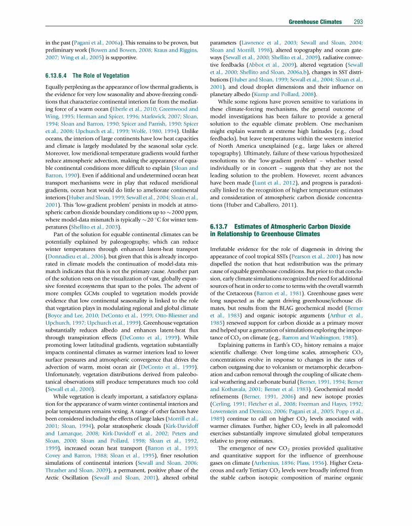
Greenhouse Climates 293

in the past (Pagani et al., 2006a). This remains to be proven, but

preliminary work (Bowen and Bowen, 2008; Kraus and Riggins,

2007; Wing et al., 2005) is supportive.

6.13.6.4 The Role of Vegetation

Equally perplexing as the appearance of low thermal gradients, is

the evidence for very low seasonality and above-freezing condi-

tions that characterize continental interiors far from the mediat-

ing force of a warm ocean (Eberle et al., 2010; Greenwood and

Wing, 1995; Herman and Spicer, 1996; Markwick, 2007; Sloan,

1994; Sloan and Barron, 1990; Spicer and Parrish, 1990; Spicer

et al., 2008; Upchurch et al., 1999; Wolfe, 1980, 1994). Unlike

oceans, the interiors of large continents have low heat capacities

and climate is largely modulated by the seasonal solar cycle.

Moreover, low meridional-temperature gradients would further

reduce atmospheric advection, making the appearance of equa-

ble continental conditions more difficult to explain (Sloan and

Barron, 1990). Even if additional and undetermined ocean heat

transport mechanisms were in play that reduced meridional

gradients, ocean heat would do little to ameliorate continental

interiors (Huber and Sloan, 1999; Sewall et al., 2004; Sloan et al.,

2001). This ‘low-gradient problem’ persists in models at atmo-

spheric carbon dioxide boundary conditions up to�2000 ppm,

where model-data mismatch is typically �20 �C for winter tem-

peratures (Shellito et al., 2003).

Part of the solution for equable continental climates can be

potentially explained by paleogeography, which can reduce

winter temperatures through enhanced latent-heat transport

(Donnadieu et al., 2006), but given that this is already incorpo-

rated in climate models the continuation of model-data mis-

match indicates that this is not the primary cause. Another part

of the solution rests on the visualization of vast, globally expan-

sive forested ecosystems that span to the poles. The advent of

more complex GCMs coupled to vegetation models provide

evidence that low continental seasonality is linked to the role

that vegetation plays in modulating regional and global climate

(Boyce and Lee, 2010; DeConto et al., 1999; Otto-Bliesner and

Upchurch, 1997; Upchurch et al., 1999). Greenhouse vegetation

substantially reduces albedo and enhances latent-heat flux

through transpiration effects (DeConto et al., 1999). While

promoting lower latitudinal gradients, vegetation substantially

impacts continental climates as warmer interiors lead to lower

surface pressures and atmospheric convergence that drives the

advection of warm, moist ocean air (DeConto et al., 1999).

Unfortunately, vegetation distributions derived from paleobo-

tanical observations still produce temperatures much too cold

(Sewall et al., 2000).

While vegetation is clearly important, a satisfactory explana-

tion for the appearance of warm winter continental interiors and

polar temperatures remains vexing. A range of other factors have

been considered including the effects of large lakes (Morrill et al.,

2001; Sloan, 1994), polar stratospheric clouds (Kirk-Davidoff

and Lamarque, 2008; Kirk-Davidoff et al., 2002; Peters and

Sloan, 2000; Sloan and Pollard, 1998; Sloan et al., 1992,

1999), increased ocean heat transport (Barron et al., 1993;

Covey and Barron, 1988; Sloan et al., 1995), finer resolution

simulations of continental interiors (Sewall and Sloan, 2006;

Thrasher and Sloan, 2009), a permanent, positive phase of the

Arctic Oscillation (Sewall and Sloan, 2001), altered orbital

parameters (Lawrence et al., 2003; Sewall and Sloan, 2004;

Sloan and Morrill, 1998), altered topography and ocean gate-

ways (Sewall et al., 2000; Shellito et al., 2009), radiative convec-

tive feedbacks (Abbot et al., 2009), altered vegetation (Sewall

et al., 2000; Shellito and Sloan, 2006a,b), changes in SST distri-

butions (Huber and Sloan, 1999; Sewall et al., 2004; Sloan et al.,

2001), and cloud droplet dimensions and their influence on

planetary albedo (Kump and Pollard, 2008).

While some regions have proven sensitive to variations in

these climate-forcing mechanisms, the general outcome of

model investigations has been failure to provide a general

solution to the equable climate problem. One mechanism

might explain warmth at extreme high latitudes (e.g., cloud

feedbacks), but leave temperatures within the western interior

of North America unexplained (e.g., large lakes or altered

topography). Ultimately, failure of these various hypothesized

resolutions to the ‘low-gradient problem’ – whether tested

individually or in concert – suggests that they are not the

leading solution to the problem. However, recent advances

have been made (Lunt et al., 2012), and progress is paradoxi-

cally linked to the recognition of higher temperature estimates

and consideration of atmospheric carbon dioxide concentra-

tions (Huber and Caballero, 2011).

6.13.7 Estimates of Atmospheric Carbon Dioxidein Relationship to Greenhouse Climates

Irrefutable evidence for the role of diagenesis in driving the

appearance of cool tropical SSTs (Pearson et al., 2001) has now

dispelled the notion that heat redistribution was the primary

cause of equable greenhouse conditions. But prior to that conclu-

sion, early climate simulations recognized theneed for additional

sources of heat in order to come to terms with the overall warmth

of the Cretaceous (Barron et al., 1981). Greenhouse gases were

long suspected as the agent driving greenhouse/icehouse cli-

mates, but results from the BLAG geochemical model (Berner

et al., 1983) and organic isotopic arguments (Arthur et al.,

1985) renewed support for carbon dioxide as a primary mover

andhelped spur a generation of simulations exploring the impor-

tance of CO2 on climate (e.g., Barron and Washington, 1985).

Explaining patterns in Earth’s CO2 history remains a major

scientific challenge. Over long-time scales, atmospheric CO2

concentrations evolve in response to changes in the rates of

carbon outgassing due to volcanism or metamorphic decarbon-

ation and carbon removal through the coupling of silicate chem-

ical weathering and carbonate burial (Berner, 1991, 1994; Berner

and Kothavala, 2001; Berner et al. 1983). Geochemical model

refinements (Berner, 1991, 2006) and new isotope proxies

(Cerling, 1991; Fletcher et al., 2008; Freeman and Hayes, 1992;

Lowenstein and Demicco, 2006; Pagani et al., 2005; Popp et al.,

1989) continue to call on higher CO2 levels associated with

warmer climates. Further, higher CO2 levels in all paleomodel

exercises substantially improve simulated global temperatures

relative to proxy estimates.

The emergence of new CO2 proxies provided qualitative

and quantitative support for the influence of greenhouse

gases on climate (Arrhenius, 1896; Plass, 1956). Higher Creta-

ceous and early Tertiary CO2 levels were broadly inferred from

the stable carbon isotopic composition of marine organic

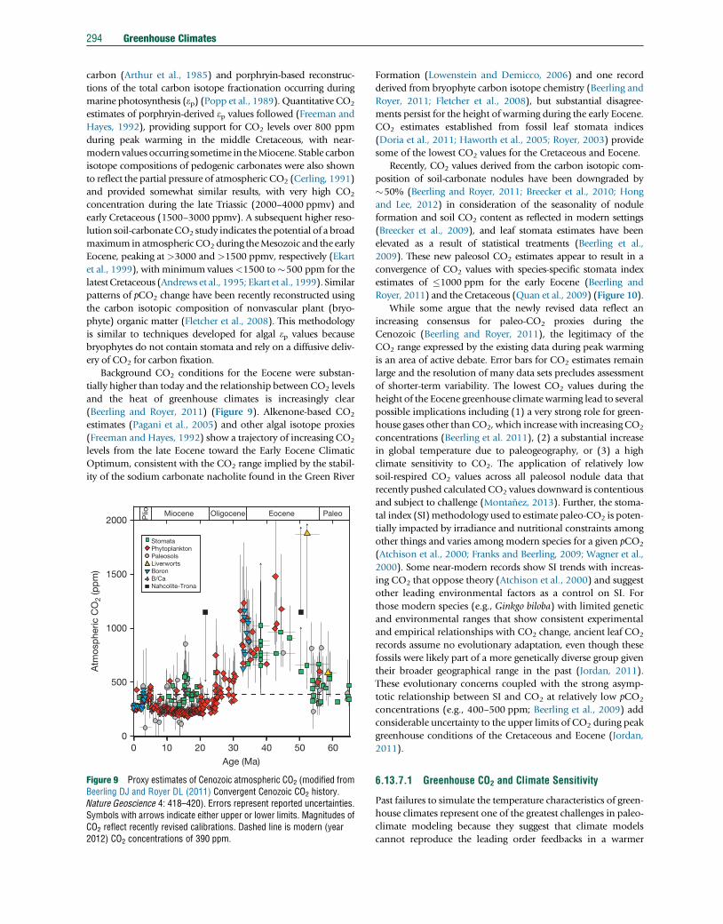
294 Greenhouse Climates

carbon (Arthur et al., 1985) and porphryin-based reconstruc-

tions of the total carbon isotope fractionation occurring during

marine photosynthesis (ep) (Popp et al., 1989). Quantitative CO2

estimates of porphryin-derived ep values followed (Freeman and

Hayes, 1992), providing support for CO2 levels over 800 ppm

during peak warming in the middle Cretaceous, with near-

modernvalues occurring sometime in theMiocene. Stable carbon

isotope compositions of pedogenic carbonates were also shown

to reflect the partial pressure of atmospheric CO2 (Cerling, 1991)

and provided somewhat similar results, with very high CO2

concentration during the late Triassic (2000–4000 ppmv) and

early Cretaceous (1500–3000 ppmv). A subsequent higher reso-

lution soil-carbonateCO2 study indicates the potential of a broad

maximum in atmospheric CO2 during theMesozoic and the early

Eocene, peaking at >3000 and >1500 ppmv, respectively (Ekart

et al., 1999), withminimum values<1500 to�500 ppm for the

latestCretaceous (Andrews et al., 1995; Ekart et al., 1999). Similar

patterns of pCO2 change have been recently reconstructed using

the carbon isotopic composition of nonvascular plant (bryo-

phyte) organic matter (Fletcher et al., 2008). This methodology

is similar to techniques developed for algal ep values because

bryophytes do not contain stomata and rely on a diffusive deliv-

ery of CO2 for carbon fixation.

Background CO2 conditions for the Eocene were substan-

tially higher than today and the relationship between CO2 levels

and the heat of greenhouse climates is increasingly clear

(Beerling and Royer, 2011) (Figure 9). Alkenone-based CO2

estimates (Pagani et al., 2005) and other algal isotope proxies

(Freeman and Hayes, 1992) show a trajectory of increasing CO2

levels from the late Eocene toward the Early Eocene Climatic

Optimum, consistent with the CO2 range implied by the stabil-

ity of the sodium carbonate nacholite found in the Green River

Atm

osp

heric

CO

2 (p

pm

)

0

500

1000

1500

2000

0 10 20 30 40 50 60

Age (Ma)

PaleoEoceneOligoceneMiocenePlio

StomataPhytoplanktonPaleosolsLiverwortsBoronB/CaNahcolite-Trona

Figure 9 Proxy estimates of Cenozoic atmospheric CO2 (modified fromBeerling DJ and Royer DL (2011) Convergent Cenozoic CO2 history.Nature Geoscience 4: 418–420). Errors represent reported uncertainties.Symbols with arrows indicate either upper or lower limits. Magnitudes ofCO2 reflect recently revised calibrations. Dashed line is modern (year2012) CO2 concentrations of 390 ppm.

Formation (Lowenstein and Demicco, 2006) and one record

derived from bryophyte carbon isotope chemistry (Beerling and

Royer, 2011; Fletcher et al., 2008), but substantial disagree-

ments persist for the height of warming during the early Eocene.

CO2 estimates established from fossil leaf stomata indices

(Doria et al., 2011; Haworth et al., 2005; Royer, 2003) provide

some of the lowest CO2 values for the Cretaceous and Eocene.

Recently, CO2 values derived from the carbon isotopic com-

position of soil-carbonate nodules have been downgraded by

�50% (Beerling and Royer, 2011; Breecker et al., 2010; Hong

and Lee, 2012) in consideration of the seasonality of nodule

formation and soil CO2 content as reflected in modern settings

(Breecker et al., 2009), and leaf stomata estimates have been

elevated as a result of statistical treatments (Beerling et al.,

2009). These new paleosol CO2 estimates appear to result in a

convergence of CO2 values with species-specific stomata index

estimates of �1000 ppm for the early Eocene (Beerling and

Royer, 2011) and the Cretaceous (Quan et al., 2009) (Figure 10).

While some argue that the newly revised data reflect an

increasing consensus for paleo-CO2 proxies during the

Cenozoic (Beerling and Royer, 2011), the legitimacy of the

CO2 range expressed by the existing data during peak warming

is an area of active debate. Error bars for CO2 estimates remain

large and the resolution of many data sets precludes assessment

of shorter-term variability. The lowest CO2 values during the

height of the Eocene greenhouse climate warming lead to several

possible implications including (1) a very strong role for green-

house gases other than CO2, which increase with increasing CO2

concentrations (Beerling et al. 2011), (2) a substantial increase

in global temperature due to paleogeography, or (3) a high

climate sensitivity to CO2. The application of relatively low

soil-respired CO2 values across all paleosol nodule data that

recently pushed calculated CO2 values downward is contentious

and subject to challenge (Montanez, 2013). Further, the stoma-

tal index (SI)methodology used to estimate paleo-CO2 is poten-

tially impacted by irradiance and nutritional constraints among

other things and varies among modern species for a given pCO2

(Atchison et al., 2000; Franks and Beerling, 2009; Wagner et al.,

2000). Some near-modern records show SI trends with increas-

ing CO2 that oppose theory (Atchison et al., 2000) and suggest

other leading environmental factors as a control on SI. For

those modern species (e.g., Ginkgo biloba) with limited genetic

and environmental ranges that show consistent experimental

and empirical relationships with CO2 change, ancient leaf CO2

records assume no evolutionary adaptation, even though these

fossils were likely part of a more genetically diverse group given

their broader geographical range in the past (Jordan, 2011).

These evolutionary concerns coupled with the strong asymp-

totic relationship between SI and CO2 at relatively low pCO2

concentrations (e.g., 400–500 ppm; Beerling et al., 2009) add

considerable uncertainty to the upper limits of CO2 during peak

greenhouse conditions of the Cretaceous and Eocene (Jordan,

2011).

6.13.7.1 Greenhouse CO2 and Climate Sensitivity

Past failures to simulate the temperature characteristics of green-

house climates represent one of the greatest challenges in paleo-

climate modeling because they suggest that climate models

cannot reproduce the leading order feedbacks in a warmer

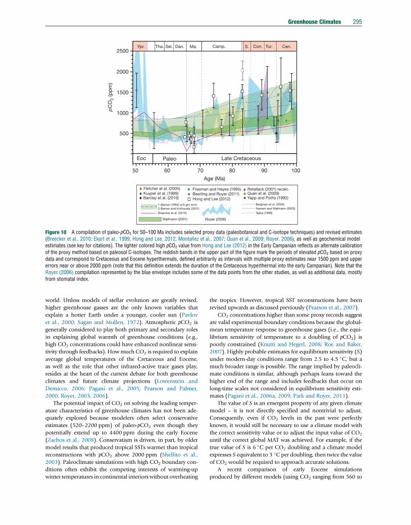
Late CretaceousPaleoEoc

Ypr. Tha. Sel. Dan. Ma. Camp.

50

500

1000

1500

2000

2500

60 70 80 90 100

2

1

Cen.Tur.Con.S.

Age (Ma)

Fletcher et al. (2005)Kuyper et al. (1999)Barclay et al. (2010)

Freeman and Hayes (1995)Beerling and Royer (2011)Hong and Lee (2012)

Bergman et al. (2004)

Royer (2006)

1-Berner (1994) w/lt grn error

Wallmann (2001)

Breecker et al. (2010)2-Berner and Kothavala (2001)

Tajika (1999)

Hansen and Wallmann (2003)

Yapp and Poths (1992)Quan et al. (2009)Retallack (2001) recalc.

pC

O2

(pp

m)

Figure 10 A compilation of paleo-pCO2 for 50–100 Ma includes selected proxy data (paleobotanical and C-isotope techniques) and revised estimates(Breecker et al., 2010; Ekart et al., 1999; Hong and Lee, 2012; Montanez et al., 2007; Quan et al., 2009; Royer, 2006), as well as geochemical modelestimates (see key for citations). The lighter colored high pCO2 value from Hong and Lee (2012) in the Early Campanian reflects an alternate calibrationof the proxy method based on paleosol C-isotopes. The reddish bands in the upper part of the figure mark the periods of elevated pCO2 based on proxydata and correspond to Cretaceous and Eocene hyperthermals, defined arbitrarily as intervals with multiple proxy estimates near 1500 ppm and uppererrors near or above 2000 ppm (note that this definition extends the duration of the Cretaceous hyperthermal into the early Campanian). Note that theRoyer (2006) compilation represented by the blue envelope includes some of the data points from the other studies, as well as additional data, mostlyfrom stomatal index.

Greenhouse Climates 295

world. Unless models of stellar evolution are greatly revised,

higher greenhouse gasses are the only known variables that

explain a hotter Earth under a younger, cooler sun (Pavlov

et al., 2000; Sagan and Mullen, 1972). Atmospheric pCO2 is

generally considered to play both primary and secondary roles

in explaining global warmth of greenhouse conditions (e.g.,

high CO2 concentrations could have enhanced nonlinear sensi-

tivity through feedbacks). Howmuch CO2 is required to explain

average global temperatures of the Cretaceous and Eocene,

as well as the role that other infrared-active trace gases play,

resides at the heart of the current debate for both greenhouse

climates and future climate projections (Lowenstein and

Demicco, 2006; Pagani et al., 2005; Pearson and Palmer,

2000; Royer, 2003, 2006).

The potential impact of CO2 on solving the leading temper-

ature characteristics of greenhouse climates has not been ade-

quately explored because modelers often select conservative

estimates (520–2200 ppm) of paleo-pCO2 even though they

potentially extend up to 4400 ppm during the early Eocene

(Zachos et al., 2008). Conservatism is driven, in part, by older

model results that produced tropical SSTs warmer than tropical

reconstructions with pCO2 above 2000 ppm (Shellito et al.,

2003). Paleoclimate simulations with high CO2 boundary con-

ditions often exhibit the competing interests of warming-up

winter temperatures in continental interiors without overheating

the tropics. However, tropical SST reconstructions have been

revised upwards as discussed previously (Pearson et al., 2007).

CO2 concentrations higher than some proxy records suggest

are valid experimental boundary conditions because the global-

mean temperature response to greenhouse gases (i.e., the equi-

librium sensitivity of temperature to a doubling of pCO2) is

poorly constrained (Knutti and Hegerl, 2008; Roe and Baker,

2007). Highly probable estimates for equilibrium sensitivity (S)

under modern-day conditions range from 2.5 to 4.5 �C, but amuch broader range is possible. The range implied by paleocli-

mate conditions is similar, although perhaps leans toward the

higher end of the range and includes feedbacks that occur on

long-time scales not considered in equilibrium sensitivity esti-

mates (Pagani et al., 2006a, 2009; Park and Royer, 2011).

The value of S is an emergent property of any given climate

model – it is not directly specified and nontrivial to adjust.

Consequently, even if CO2 levels in the past were perfectly

known, it would still be necessary to use a climate model with

the correct sensitivity value or to adjust the input value of CO2

until the correct global MAT was achieved. For example, if the

true value of S is 6 �C per CO2 doubling and a climate model

expresses S equivalent to 3 �C per doubling, then twice the value

of CO2 would be required to approach accurate solutions.

A recent comparison of early Eocene simulations

produced by different models (using CO2 ranging from 560 to

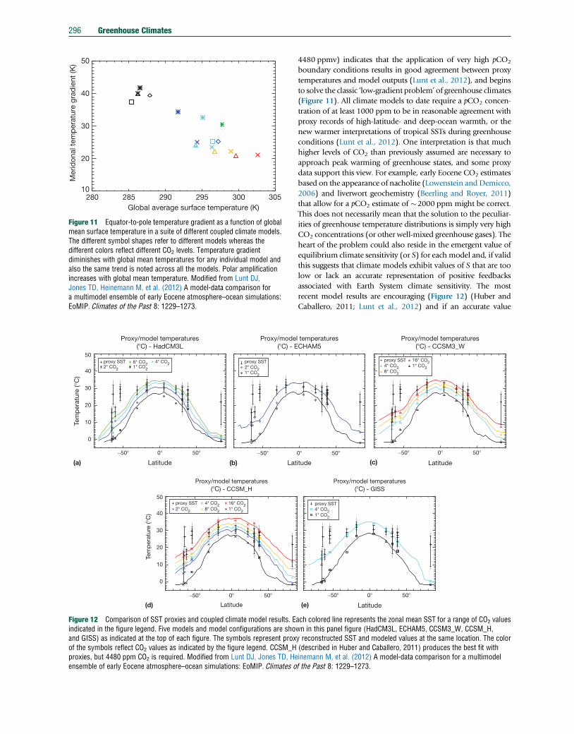
280 285 290 295 300 305Global average surface temperature (K)

10

20

30

40

50

Mer

idon

al t

emp

erat

ure

grad

ient

(K)

Figure 11 Equator-to-pole temperature gradient as a function of globalmean surface temperature in a suite of different coupled climate models.The different symbol shapes refer to different models whereas thedifferent colors reflect different CO2 levels. Temperature gradientdiminishes with global mean temperatures for any individual model andalso the same trend is noted across all the models. Polar amplificationincreases with global mean temperature. Modified from Lunt DJ,Jones TD, Heinemann M, et al. (2012) A model-data comparison fora multimodel ensemble of early Eocene atmosphere–ocean simulations:EoMIP. Climates of the Past 8: 1229–1273.

Proxy/model temperatures(�C) - HadCM3L

-50� 0� 50�

Latitude

0

10

20

30

40

50

2* CO2

4* CO26* CO21* CO2

proxy SST

(a)

Proxy/mode(�C) - E

-50�

Lat

2* CO21* CO2

proxy SST

(b)

(d)

Proxy/model temperatures(�C) - CCSM_H

2* CO2

4* CO28* CO2

16* CO21* CO2

proxy SST

Tem

per

atur

e (°

C)

-50� 0� 50�

Latitude

0

10

20

30

40

50

Tem

per

atur

e (°

C)

Figure 12 Comparison of SST proxies and coupled climate model results. Eindicated in the figure legend. Five models and model configurations are shoand GISS) as indicated at the top of each figure. The symbols represent proxof the symbols reflect CO2 values as indicated by the figure legend. CCSM_Hproxies, but 4480 ppm CO2 is required. Modified from Lunt DJ, Jones TD, Heensemble of early Eocene atmosphere–ocean simulations: EoMIP. Climates o

296 Greenhouse Climates

4480 ppmv) indicates that the application of very high pCO2

boundary conditions results in good agreement between proxy

temperatures and model outputs (Lunt et al., 2012), and begins

to solve the classic ‘low-gradient problem’ of greenhouse climates

(Figure 11). All climate models to date require a pCO2 concen-

tration of at least 1000 ppm to be in reasonable agreement with

proxy records of high-latitude- and deep-ocean warmth, or the

new warmer interpretations of tropical SSTs during greenhouse

conditions (Lunt et al., 2012). One interpretation is that much

higher levels of CO2 than previously assumed are necessary to

approach peak warming of greenhouse states, and some proxy

data support this view. For example, early Eocene CO2 estimates

based on the appearance of nacholite (Lowenstein and Demicco,

2006) and liverwort geochemistry (Beerling and Royer, 2011)

that allow for a pCO2 estimate of �2000 ppm might be correct.

This does not necessarily mean that the solution to the peculiar-

ities of greenhouse temperature distributions is simply very high

CO2 concentrations (or other well-mixed greenhouse gases). The

heart of the problem could also reside in the emergent value of

equilibrium climate sensitivity (or S) for eachmodel and, if valid

this suggests that climate models exhibit values of S that are too

low or lack an accurate representation of positive feedbacks

associated with Earth System climate sensitivity. The most

recent model results are encouraging (Figure 12) (Huber and

Caballero, 2011; Lunt et al., 2012) and if an accurate value

l temperaturesCHAM5

0� 50�

itude (c)

(e)

Proxy/model temperatures(�C) - CCSM3_W

4* CO28* CO2

16* CO21* CO2

proxy SST

Proxy/model temperatures(�C) - GISS

4* CO21* CO2

proxy SST

-50� 0� 50�

Latitude

-50� 0� 50�

Latitude

ach colored line represents the zonal mean SST for a range of CO2 valueswn in this panel figure (HadCM3L, ECHAM5, CCSM3_W, CCSM_H,y reconstructed SST and modeled values at the same location. The color(described in Huber and Caballero, 2011) produces the best fit withinemann M, et al. (2012) A model-data comparison for a multimodelf the Past 8: 1229–1273.

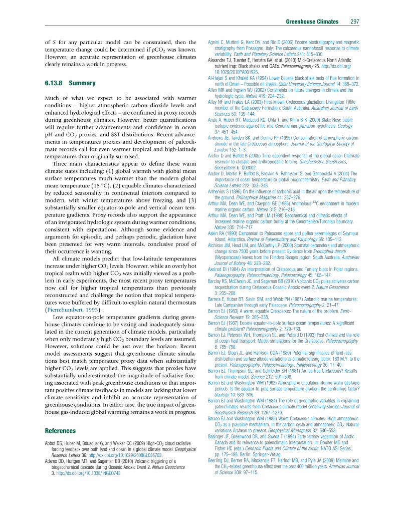
Greenhouse Climates 297

of S for any particular model can be constrained, then the

temperature change could be determined if pCO2 was known.

However, an accurate representation of greenhouse climates

clearly remains a work in progress.

6.13.8 Summary

Much of what we expect to be associated with warmer

conditions – higher atmospheric carbon dioxide levels and

enhanced hydrological effects – are confirmed in proxy records

during greenhouse climates. However, better quantifications

will require further advancements and confidence in ocean

pH and CO2 proxies, and SST distributions. Recent advance-

ments in temperatures proxies and development of paleocli-

mate records call for even warmer tropical and high-latitude

temperatures than originally surmised.

Three main characteristics appear to define these warm

climate states including: (1) global warmth with global mean

surface temperatures much warmer than the modern global

mean temperature (15 �C), (2) equable climates characterized

by reduced seasonality in continental interiors compared to

modern, with winter temperatures above freezing, and (3)

substantially smaller equator-to-pole and vertical ocean tem-

perature gradients. Proxy records also support the appearance

of an invigorated hydrologic system during warmer conditions,

consistent with expectations. Although some evidence and

arguments for episodic, and perhaps periodic, glaciation have

been presented for very warm intervals, conclusive proof of

their occurrence is wanting.

All climate models predict that low-latitude temperatures

increase under higher CO2 levels. However, while an overly hot

tropical realm with higher CO2 was initially viewed as a prob-

lem in early experiments, the most recent proxy temperatures

now call for higher tropical temperatures than previously

reconstructed and challenge the notion that tropical tempera-

tures were buffered by difficult-to-explain natural thermostats

(Pierrehumbert, 1995).

Low equator-to-pole temperature gradients during green-

house climates continue to be vexing and inadequately simu-

lated in the current generation of climate models, particularly

when only moderately high CO2 boundary levels are assumed.

However, solutions could be just over the horizon. Recent

model assessments suggest that greenhouse climate simula-

tions best match temperature proxy data when substantially

higher CO2 levels are applied. This suggests that proxies have

substantially underestimated the magnitude of radiative forc-

ing associated with peak greenhouse conditions or that impor-

tant positive climate feedbacks in models are lacking that lower

climate sensitivity and inhibit an accurate representation of

greenhouse conditions. In either case, the true impact of green-

house gas-induced global warming remains a work in progress.

References

Abbot DS, Huber M, Bousquet G, and Walker CC (2009) High-CO2 cloud radiativeforcing feedback over both land and ocean in a global climate model. GeophysicalResearch Letters 36. http://dx.doi.org/10.1029/2008GL036703.

Adams DD, Hurtgen MT, and Sageman BB (2010) Volcanic triggering of abiogeochemical cascade during Oceanic Anoxic Event 2. Nature Geoscience3. http://dx.doi.org/10.1038/ NGEO743

Agnini C, Muttoni G, Kent DV, and Rio D (2006) Eocene biostratigraphy and magneticstratigraphy from Possagno, Italy: The calcareous nannofossil response to climatevariability. Earth and Planetary Science Letters 241: 815–830.

Alexandre TJ, Tuenter E, Henstra GA, et al. (2010) Mid-Cretaceous North Atlanticnutrient trap: Black shales and OAEs. Paleoceanography 25. http://dx.doi.org/10.1029/2010PA001925.

Al-Hajari S and Khaled KA (1994) Lower Eocene black shale beds of Rus formation innorth of Oman – Possible oil shales. Qatar University Science Journal 14: 368–372.

Allen MR and Ingram WJ (2002) Constraints on future changes in climate and thehydrologic cycle. Nature 419: 224–232.

Alley NF and Frakes LA (2003) First known Cretaceous glaciation: Livingston Tillitemember of the Cadnaowie Formation, South Australia. Australian Journal of EarthSciences 50: 139–144.

Ando A, Huber BT, MacLeod KG, Ohta T, and Khim B-K (2009) Blake Nose stableisotopic evidence against the mid-Cenomanian glaciation hypothesis. Geology37: 451–454.

Andrews JE, Tanden SK, and Dennis PF (1995) Concentration of atmospheric carbondioxide in the late Cretaceous atmosphere. Journal of the Geological Society ofLondon 152: 1–3.

Archer D and Buffett B (2005) Time-dependent response of the global ocean Clathratereservoir to climatic and anthropogenic forcing. Geochemistry, Geophysics,Geosystems 6: Q03002.

Archer D, Martin P, Buffett B, Brovkin V, Rahmstorf S, and Ganopolski A (2004) Theimportance of ocean temperature to global biogeochemistry. Earth and PlanetaryScience Letters 222: 333–348.

Arrhenius S (1896) On the influence of carbonic acid in the air upon the temperature ofthe ground. Philosphical Magazine 41: 237–276.

Arthur MA, Dean WE, and Claypool GE (1985) Anomalous 13C enrichment in modernmarine organic carbon. Nature 315: 216–218.

Arthur MA, Dean WE, and Pratt LM (1988) Geochemical and climatic effects ofincreased marine organic carbon burial at the Cenomanian/Turonian boundary.Nature 335: 714–717.

Askin RA (1990) Campanian to Paleocene spore and pollen assemblages of SeymourIsland, Antarctica. Review of Palaeobotany and Palynology 65: 105–113.

Atchison JM, Head LM, and McCarthy LP (2000) Stomatal parameters and atmosphericchange since 7500 years before present: Evidence from Eremophila deserti(Myoporaceae) leaves from the Flinders Ranges region, South Australia. AustralianJournal of Botany 48: 223–232.

Axelrod DI (1984) An interpretation of Cretaceous and Tertiary biota in Polar regions.Palaeogeography, Palaeoclimatology, Palaeoecology 45: 105–147.

Barclay RS, McElwain JC, and Sageman BB (2010) Volcanic CO2 pulse activates carbonsequestration during Cretaceous Oceanic Anoxic event 2. Nature Geoscience3: 205–208.

Barrera E, Huber BT, Savin SM, and Webb PN (1987) Antarctic marine temperatures:Late Campanian through early Paleocene. Paleoceanography 2: 21–47.

Barron EJ (1983) A warm, equable Cretaceous: The nature of the problem. Earth-Science Reviews 19: 305–338.

Barron EJ (1987) Eocene equator-to-pole surface ocean temperatures: A significantclimate problem? Paleoceanography 2: 729–739.

Barron EJ, Peterson WH, Thompson SL, and Pollard D (1993) Past climate and the roleof ocean heat transport: Model simulations for the Cretaceous. Paleoceanography8: 785–798.

Barron EJ, Sloan JL, and Harrison CGA (1980) Potential significance of land–seadistribution and surface albedo variations as climatic forcing factor: 180 M.Y. to thepresent. Palaeogeography, Palaeoclimatology, Palaeoecology 30: 17–40.

Barron EJ, Thompson SL, and Schneider SH (1981) An ice-free Cretaceous? Resultsfrom climate model. Science 212: 501–508.

Barron EJ and Washington WM (1982) Atmospheric circulation during warm geologicperiods: Is the equator-to-pole surface temperature gradient the controlling factor?Geology 10: 633–636.

Barron EJ and Washington WM (1984) The role of geographic variables in explainingpaleoclimates results from Cretaceous climate model sensitivity studies. Journal ofGeophysical Research 89: 1267–1279.

Barron EJ and Washington WM (1985) Warm Cretaceous climates: High atmosphericCO2 as a plausible mechanism. In the carbon cycle and atmospheric CO2: Naturalvariations Archean to present. Geophysical Monograph 32: 546–553.

Basinger JF, Greenwood DR, and Sweda T (1994) Early tertiary vegetation of ArcticCanada and its relevance to paleoclimatic interpretation. In: Boulter MC andFisher HC (eds.) Cenozoic Plants and Climate of the Arctic. NATO ASI Series,pp. 175–198. Berlin: Springer-Verlag.

Beerling DJ, Berner RA, Mackenzie FT, Harfoot MB, and Pyle JA (2009) Methane andthe CH4-related greenhouse effect over the past 400 million years. American Journalof Science 309: 97–115.

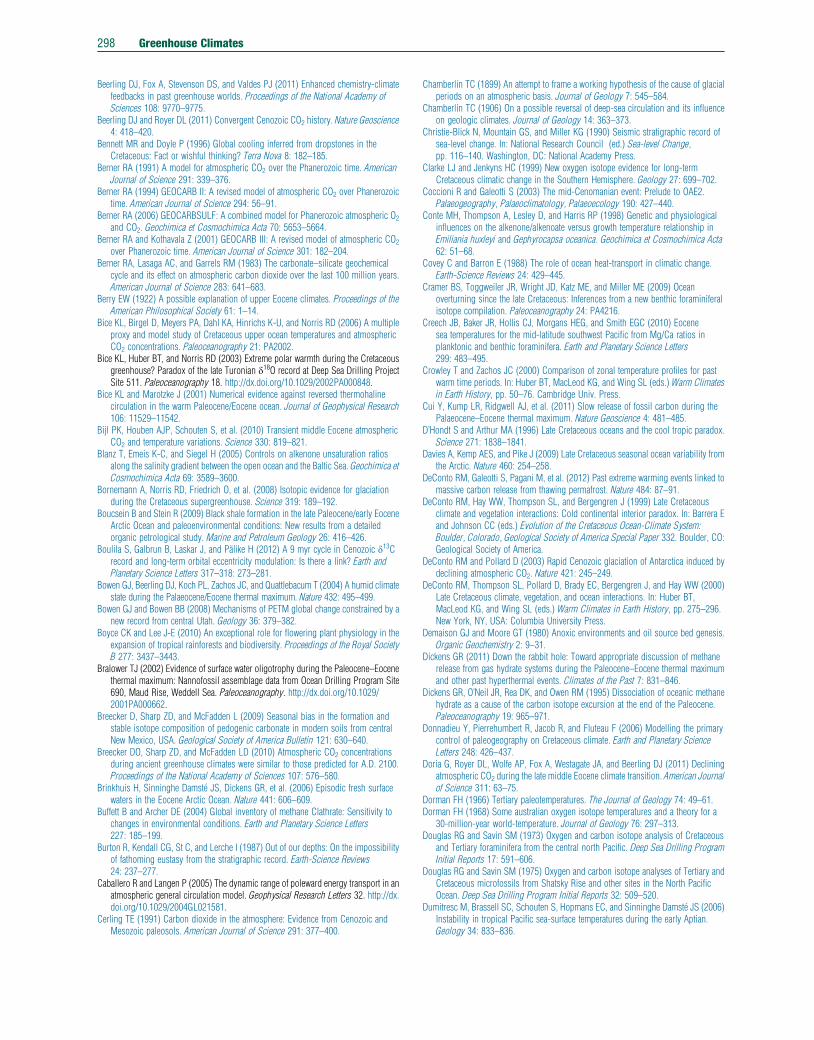
298 Greenhouse Climates

Beerling DJ, Fox A, Stevenson DS, and Valdes PJ (2011) Enhanced chemistry-climatefeedbacks in past greenhouse worlds. Proceedings of the National Academy ofSciences 108: 9770–9775.

Beerling DJ and Royer DL (2011) Convergent Cenozoic CO2 history. Nature Geoscience4: 418–420.

Bennett MR and Doyle P (1996) Global cooling inferred from dropstones in theCretaceous: Fact or wishful thinking? Terra Nova 8: 182–185.

Berner RA (1991) A model for atmospheric CO2 over the Phanerozoic time. AmericanJournal of Science 291: 339–376.

Berner RA (1994) GEOCARB II: A revised model of atmospheric CO2 over Phanerozoictime. American Journal of Science 294: 56–91.

Berner RA (2006) GEOCARBSULF: A combined model for Phanerozoic atmospheric O2and CO2. Geochimica et Cosmochimica Acta 70: 5653–5664.

Berner RA and Kothavala Z (2001) GEOCARB III: A revised model of atmospheric CO2over Phanerozoic time. American Journal of Science 301: 182–204.

Berner RA, Lasaga AC, and Garrels RM (1983) The carbonate–silicate geochemicalcycle and its effect on atmospheric carbon dioxide over the last 100 million years.American Journal of Science 283: 641–683.

Berry EW (1922) A possible explanation of upper Eocene climates. Proceedings of theAmerican Philosophical Society 61: 1–14.

Bice KL, Birgel D, Meyers PA, Dahl KA, Hinrichs K-U, and Norris RD (2006) A multipleproxy and model study of Cretaceous upper ocean temperatures and atmosphericCO2 concentrations. Paleoceanography 21: PA2002.

Bice KL, Huber BT, and Norris RD (2003) Extreme polar warmth during the Cretaceousgreenhouse? Paradox of the late Turonian d18O record at Deep Sea Drilling ProjectSite 511. Paleoceanography 18. http://dx.doi.org/10.1029/2002PA000848.

Bice KL and Marotzke J (2001) Numerical evidence against reversed thermohalinecirculation in the warm Paleocene/Eocene ocean. Journal of Geophysical Research106: 11529–11542.

Bijl PK, Houben AJP, Schouten S, et al. (2010) Transient middle Eocene atmosphericCO2 and temperature variations. Science 330: 819–821.

Blanz T, Emeis K-C, and Siegel H (2005) Controls on alkenone unsaturation ratiosalong the salinity gradient between the open ocean and the Baltic Sea. Geochimica etCosmochimica Acta 69: 3589–3600.

Bornemann A, Norris RD, Friedrich O, et al. (2008) Isotopic evidence for glaciationduring the Cretaceous supergreenhouse. Science 319: 189–192.

Boucsein B and Stein R (2009) Black shale formation in the late Paleocene/early EoceneArctic Ocean and paleoenvironmental conditions: New results from a detailedorganic petrological study. Marine and Petroleum Geology 26: 416–426.

Boulila S, Galbrun B, Laskar J, and Palike H (2012) A 9 myr cycle in Cenozoic d13Crecord and long-term orbital eccentricity modulation: Is there a link? Earth andPlanetary Science Letters 317–318: 273–281.

Bowen GJ, Beerling DJ, Koch PL, Zachos JC, and Quattlebacum T (2004) A humid climatestate during the Palaeocene/Eocene thermal maximum. Nature 432: 495–499.

Bowen GJ and Bowen BB (2008) Mechanisms of PETM global change constrained by anew record from central Utah. Geology 36: 379–382.

Boyce CK and Lee J-E (2010) An exceptional role for flowering plant physiology in theexpansion of tropical rainforests and biodiversity. Proceedings of the Royal SocietyB 277: 3437–3443.

Bralower TJ (2002) Evidence of surface water oligotrophy during the Paleocene–Eocenethermal maximum: Nannofossil assemblage data from Ocean Drilling Program Site690, Maud Rise, Weddell Sea. Paleoceanography. http://dx.doi.org/10.1029/2001PA000662.

Breecker D, Sharp ZD, and McFadden L (2009) Seasonal bias in the formation andstable isotope composition of pedogenic carbonate in modern soils from centralNew Mexico, USA. Geological Society of America Bulletin 121: 630–640.

Breecker DO, Sharp ZD, and McFadden LD (2010) Atmospheric CO2 concentrationsduring ancient greenhouse climates were similar to those predicted for A.D. 2100.Proceedings of the National Academy of Sciences 107: 576–580.

Brinkhuis H, Sinninghe Damste JS, Dickens GR, et al. (2006) Episodic fresh surfacewaters in the Eocene Arctic Ocean. Nature 441: 606–609.

Buffett B and Archer DE (2004) Global inventory of methane Clathrate: Sensitivity tochanges in environmental conditions. Earth and Planetary Science Letters227: 185–199.

Burton R, Kendall CG, St C, and Lerche I (1987) Out of our depths: On the impossibilityof fathoming eustasy from the stratigraphic record. Earth-Science Reviews24: 237–277.

Caballero R and Langen P (2005) The dynamic range of poleward energy transport in anatmospheric general circulation model. Geophysical Research Letters 32. http://dx.doi.org/10.1029/2004GL021581.

Cerling TE (1991) Carbon dioxide in the atmosphere: Evidence from Cenozoic andMesozoic paleosols. American Journal of Science 291: 377–400.

Chamberlin TC (1899) An attempt to frame a working hypothesis of the cause of glacialperiods on an atmospheric basis. Journal of Geology 7: 545–584.

Chamberlin TC (1906) On a possible reversal of deep-sea circulation and its influenceon geologic climates. Journal of Geology 14: 363–373.

Christie-Blick N, Mountain GS, and Miller KG (1990) Seismic stratigraphic record ofsea-level change. In: National Research Council (ed.) Sea-level Change,pp. 116–140. Washington, DC: National Academy Press.

Clarke LJ and Jenkyns HC (1999) New oxygen isotope evidence for long-termCretaceous climatic change in the Southern Hemisphere. Geology 27: 699–702.

Coccioni R and Galeotti S (2003) The mid-Cenomanian event: Prelude to OAE2.Palaeogeography, Palaeoclimatology, Palaeoecology 190: 427–440.

Conte MH, Thompson A, Lesley D, and Harris RP (1998) Genetic and physiologicalinfluences on the alkenone/alkenoate versus growth temperature relationship inEmiliania huxleyi and Gephyrocapsa oceanica. Geochimica et Cosmochimica Acta62: 51–68.

Covey C and Barron E (1988) The role of ocean heat-transport in climatic change.Earth-Science Reviews 24: 429–445.

Cramer BS, Toggweiler JR, Wright JD, Katz ME, and Miller ME (2009) Oceanoverturning since the late Cretaceous: Inferences from a new benthic foraminiferalisotope compilation. Paleoceanography 24: PA4216.

Creech JB, Baker JR, Hollis CJ, Morgans HEG, and Smith EGC (2010) Eocenesea temperatures for the mid-latitude southwest Pacific from Mg/Ca ratios inplanktonic and benthic foraminifera. Earth and Planetary Science Letters299: 483–495.

Crowley T and Zachos JC (2000) Comparison of zonal temperature profiles for pastwarm time periods. In: Huber BT, MacLeod KG, and Wing SL (eds.) Warm Climatesin Earth History, pp. 50–76. Cambridge Univ. Press.

Cui Y, Kump LR, Ridgwell AJ, et al. (2011) Slow release of fossil carbon during thePalaeocene–Eocene thermal maximum. Nature Geoscience 4: 481–485.

D’Hondt S and Arthur MA (1996) Late Cretaceous oceans and the cool tropic paradox.Science 271: 1838–1841.

Davies A, Kemp AES, and Pike J (2009) Late Cretaceous seasonal ocean variability fromthe Arctic. Nature 460: 254–258.

DeConto RM, Galeotti S, Pagani M, et al. (2012) Past extreme warming events linked tomassive carbon release from thawing permafrost. Nature 484: 87–91.

DeConto RM, Hay WW, Thompson SL, and Bergengren J (1999) Late Cretaceousclimate and vegetation interactions: Cold continental interior paradox. In: Barrera Eand Johnson CC (eds.) Evolution of the Cretaceous Ocean-Climate System:Boulder, Colorado, Geological Society of America Special Paper 332. Boulder, CO:Geological Society of America.

DeConto RM and Pollard D (2003) Rapid Cenozoic glaciation of Antarctica induced bydeclining atmospheric CO2. Nature 421: 245–249.

DeConto RM, Thompson SL, Pollard D, Brady EC, Bergengren J, and Hay WW (2000)Late Cretaceous climate, vegetation, and ocean interactions. In: Huber BT,MacLeod KG, and Wing SL (eds.) Warm Climates in Earth History, pp. 275–296.New York, NY, USA: Columbia University Press.

Demaison GJ and Moore GT (1980) Anoxic environments and oil source bed genesis.Organic Geochemistry 2: 9–31.

Dickens GR (2011) Down the rabbit hole: Toward appropriate discussion of methanerelease from gas hydrate systems during the Paleocene–Eocene thermal maximumand other past hyperthermal events. Climates of the Past 7: 831–846.

Dickens GR, O’Neil JR, Rea DK, and Owen RM (1995) Dissociation of oceanic methanehydrate as a cause of the carbon isotope excursion at the end of the Paleocene.Paleoceanography 19: 965–971.

Donnadieu Y, Pierrehumbert R, Jacob R, and Fluteau F (2006) Modelling the primarycontrol of paleogeography on Cretaceous climate. Earth and Planetary ScienceLetters 248: 426–437.

Doria G, Royer DL, Wolfe AP, Fox A, Westagate JA, and Beerling DJ (2011) Decliningatmospheric CO2 during the late middle Eocene climate transition. American Journalof Science 311: 63–75.

Dorman FH (1966) Tertiary paleotemperatures. The Journal of Geology 74: 49–61.Dorman FH (1968) Some australian oxygen isotope temperatures and a theory for a

30-million-year world-temperature. Journal of Geology 76: 297–313.Douglas RG and Savin SM (1973) Oxygen and carbon isotope analysis of Cretaceous

and Tertiary foraminifera from the central north Pacific. Deep Sea Drilling ProgramInitial Reports 17: 591–606.

Douglas RG and Savin SM (1975) Oxygen and carbon isotope analyses of Tertiary andCretaceous microfossils from Shatsky Rise and other sites in the North PacificOcean. Deep Sea Drilling Program Initial Reports 32: 509–520.

Dumitresc M, Brassell SC, Schouten S, Hopmans EC, and Sinninghe Damste JS (2006)Instability in tropical Pacific sea-surface temperatures during the early Aptian.Geology 34: 833–836.

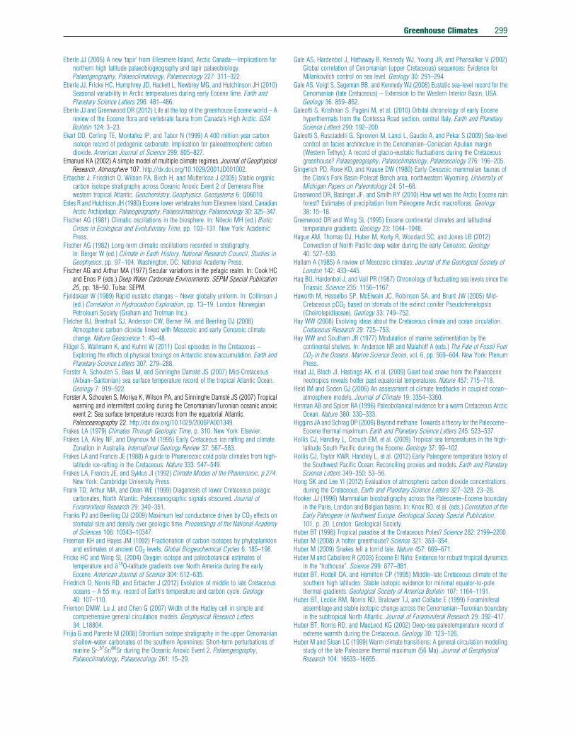
Greenhouse Climates 299

Eberle JJ (2005) A new ‘tapir’ from Ellesmere Island, Arctic Canada—Implications fornorthern high latitude palaeobiogeography and tapir palaeobiology.Palaeogeography, Palaeoclimatology, Palaeoecology 227: 311–322.

Eberle JJ, Fricke HC, Humphrey JD, Hackett L, Newbrey MG, and Hutchinson JH (2010)Seasonal variability in Arctic temperatures during early Eocene time. Earth andPlanetary Science Letters 296: 481–486.

Eberle JJ and Greenwood DR (2012) Life at the top of the greenhouse Eocene world – Areview of the Eocene flora and vertebrate fauna from Canada’s High Arctic. GSABulletin 124: 3–23.

Ekart DD, Cerling TE, Montanez IP, and Tabor N (1999) A 400 million year carbonisotope record of pedogenic carbonate: Implication for paleoatmospheric carbondioxide. American Journal of Science 299: 805–827.

Emanuel KA (2002) A simple model of multiple climate regimes. Journal of GeophysicalResearch, Atmosphere 107. http://dx.doi.org/10.1029/2001JD001002.

Erbacher J, Friedrich O, Wilson PA, Birch H, and Mutterlose J (2005) Stable organiccarbon isotope stratigraphy across Oceanic Anoxic Event 2 of Demerara Risewestern tropical Atlantic. Geochemistry, Geophysics. Geosystems 6: Q06010.

Estes R and Hutchison JH (1980) Eocene lower vertebrates from Ellesmere Island, CanadianArctic Archipelago. Palaeogeography, Palaeoclimatology, Palaeoecology 30: 325–347.

Fischer AG (1981) Climatic oscillations in the biosphere. In: Nitecki MH (ed.) BioticCrises in Ecological and Evolutionary Time, pp. 103–131. New York: AcademicPress.

Fischer AG (1982) Long-term climatic oscillations recorded in stratigraphy.In: Berger W (ed.) Climate in Earth History. National Research Council, Studies inGeophysics, pp. 97–104. Washington, DC: National Academy Press.

Fischer AG and Arthur MA (1977) Secular variations in the pelagic realm. In: Cook HCand Enos P (eds.) Deep Water Carbonate Environments. SEPM Special Publication25, pp. 18–50. Tulsa: SEPM.

Fjeldskaar W (1989) Rapid eustatic changes – Never globally uniform. In: Collinson J(ed.) Correlation in Hydrocarbon Exploration, pp. 13–19. London: NorwegianPetroleum Society (Graham and Trotman Inc.).

Fletcher BJ, Brentnall SJ, Anderson CW, Berner RA, and Beerling DJ (2008)Atmospheric carbon dioxide linked with Mesozoic and early Cenozoic climatechange. Nature Geoscience 1: 43–48.

Flogel S, Wallmann K, and Kuhnt W (2011) Cool episodes in the Cretaceous –Exploring the effects of physical forcings on Antarctic snow accumulation. Earth andPlanetary Science Letters 307: 279–288.

Forster A, Schouten S, Baas M, and Sinninghe Damste JS (2007) Mid-Cretaceous(Albian–Santonian) sea surface temperature record of the tropical Atlantic Ocean.Geology 7: 919–922.

Forster A, Schouten S, Moriya K, Wilson PA, and Sinninghe Damste JS (2007) Tropicalwarming and intermittent cooling during the Cenomanian/Turonian oceanic anoxicevent 2: Sea surface temperature records from the equatorial Atlantic.Paleoceanography 22. http://dx.doi.org/10.1029/2006PA001349.

Frakes LA (1979) Climates Through Geologic Time, p. 310. New York: Elsevier.Frakes LA, Alley NF, and Deynoux M (1995) Early Cretaceous ice rafting and climate

Zonation in Australia. International Geology Review 37: 567–583.Frakes LA and Francis JE (1988) A guide to Phanerozoic cold polar climates from high-

latitude ice-rafting in the Cretaceous. Nature 333: 547–549.Frakes LA, Francis JE, and Syktus JI (1992) Climate Modes of the Phanerozoic, p 274.

New York: Cambridge University Press.Frank TD, Arthur MA, and Dean WE (1999) Diagenesis of lower Cretaceous pelagic

carbonates, North Atlantic: Paleoceanographic signals obscured. Journal ofForaminiferal Research 29: 340–351.

Franks PJ and Beerling DJ (2009) Maximum leaf conductance driven by CO2 effects onstomatal size and density over geologic time. Proceedings of the National Academyof Sciences 106: 10343–10347.

Freeman KH and Hayes JM (1992) Fractionation of carbon isotopes by phytoplanktonand estimates of ancient CO2 levels. Global Biogeochemical Cycles 6: 185–198.

Fricke HC and Wing SL (2004) Oxygen isotope and paleobotanical estimates oftemperature and d18O-latitude gradients over North America during the earlyEocene. American Journal of Science 304: 612–635.

Friedrich O, Norris RD, and Erbacher J (2012) Evolution of middle to late Cretaceousoceans – A 55 m.y. record of Earth’s temperature and carbon cycle. Geology40: 107–110.

Frierson DMW, Lu J, and Chen G (2007) Width of the Hadley cell in simple andcomprehensive general circulation models. Geophysical Research Letters34: L18804.

Frijia G and Parente M (2008) Strontium isotope stratigraphy in the upper Cenomanianshallow-water carbonates of the southern Apennines: Short-term perturbations ofmarine Sr-87Sr/86Sr during the Oceanic Anoxic Event 2. Palaeogeography,Palaeoclimatology, Palaeoecology 261: 15–29.

Gale AS, Hardenbol J, Hathaway B, Kennedy WJ, Young JR, and Phansalkar V (2002)Global correlation of Cenomanian (upper Cretaceous) sequences: Evidence forMilankovitch control on sea level. Geology 30: 291–294.

Gale AS, Voigt S, Sageman BB, and Kennedy WJ (2008) Eustatic sea-level record for theCenomanian (late Cretaceous) – Extension to the Western Interior Basin, USA.Geology 36: 859–862.

Galeotti S, Krishnan S, Pagani M, et al. (2010) Orbital chronology of early Eocenehyperthermals from the Contessa Road section, central Italy. Earth and PlanetaryScience Letters 290: 192–200.

Galeotti S, Rusciadelli G, Sprovieri M, Lanci L, Gaudio A, and Pekar S (2009) Sea-levelcontrol on facies architecture in the Cenomanian–Coniacian Apulian margin(Western Tethys): A record of glacio-eustatic fluctuations during the Cretaceousgreenhouse? Palaeogeography, Palaeoclimatology, Palaeoecology 276: 196–205.

Gingerich PD, Rose KD, and Krause DW (1980) Early Cenozoic mammalian faunas ofthe Clark’s Fork Basin-Polecat Bench area, northwestern Wyoming. University ofMichigan Papers on Paleontology 24: 51–68.

Greenwood DR, Basinger JF, and Smith RY (2010) How wet was the Arctic Eocene rainforest? Estimates of precipitation from Paleogene Arctic macrofloras. Geology38: 15–18.

Greenwood DR and Wing SL (1995) Eocene continental climates and latitudinaltemperature gradients. Geology 23: 1044–1048.

Hague AM, Thomas DJ, Huber M, Korty R, Woodard SC, and Jones LB (2012)Convection of North Pacific deep water during the early Cenozoic. Geology40: 527–530.

Hallam A (1985) A review of Mesozoic climates. Journal of the Geological Society ofLondon 142: 433–445.

Haq BU, Hardenbol J, and Vail PR (1987) Chronology of fluctuating sea levels since theTriassic. Science 235: 1156–1167.

Haworth M, Hesselbo SP, McElwain JC, Robinson SA, and Brunt JW (2005) Mid-Cretaceous pCO2 based on stomata of the extinct conifer Pseudofrenelopsis(Cheirolepidiaceae). Geology 33: 749–752.

Hay WW (2008) Evolving ideas about the Cretaceous climate and ocean circulation.Cretaceous Research 29: 725–753.

Hay WW and Southam JR (1977) Modulation of marine sedimentation by thecontinental shelves. In: Anderson NR and Malahoff A (eds.) The Fate of Fossil FuelCO2 in the Oceans. Marine Science Series, vol. 6, pp. 569–604. New York: PlenumPress.

Head JJ, Bloch JI, Hastings AK, et al. (2009) Giant boid snake from the Palaeoceneneotropics reveals hotter past equatorial temperatures. Nature 457: 715–718.

Held IM and Soden GJ (2006) An assessment of climate feedbacks in coupled ocean–atmosphere models. Journal of Climate 19: 3354–3360.

Herman AB and Spicer RA (1996) Paleobotanical evidence for a warm Cretaceous ArcticOcean. Nature 380: 330–333.

Higgins JA and Schrag DP (2006) Beyond methane: Towards a theory for the Paleocene–Eocene thermal maximum. Earth and Planetary Science Letters 245: 523–537.

Hollis CJ, Handley L, Crouch EM, et al. (2009) Tropical sea temperatures in the high-latitude South Pacific during the Eocene. Geology 37: 99–102.

Hollis CJ, Taylor KWR, Handley L, et al. (2012) Early Paleogene temperature history ofthe Southwest Pacific Ocean: Reconciling proxies and models. Earth and PlanetaryScience Letters 349–350: 53–56.

Hong SK and Lee YI (2012) Evaluation of atmospheric carbon dioxide concentrationsduring the Cretaceous. Earth and Planetary Science Letters 327–328: 23–28.

Hooker JJ (1996) Mammalian biostratigraphy across the Paleocene–Eocene boundaryin the Paris, London and Belgian basins. In: Knox RO, et al. (eds.) Correlation of theEarly Paleogene in Northwest Europe. Geological Society Special Publication,101, p. 20. London: Geological Society.

Huber BT (1998) Tropical paradise at the Cretaceous Poles? Science 282: 2199–2200.Huber M (2008) A hotter greenhouse? Science 321: 353–354.Huber M (2009) Snakes tell a torrid tale. Nature 457: 669–671.Huber M and Caballero R (2003) Eocene El Nino: Evidence for robust tropical dynamics

in the “hothouse”. Science 299: 877–881.Huber BT, Hodell DA, and Hamilton CP (1995) Middle–late Cretaceous climate of the

southern high latitudes: Stable isotopic evidence for minimal equator-to-polethermal gradients. Geological Society of America Bulletin 107: 1164–1191.

Huber BT, Leckie RM, Norris RD, Bralower TJ, and CoBabe E (1999) Foraminiferalassemblage and stable isotopic change across the Cenomanian–Turonian boundaryin the subtropical North Atlantic. Journal of Foraminiferal Research 29: 392–417.

Huber BT, Norris RD, and MacLeod KG (2002) Deep-sea paleotemperature record ofextreme warmth during the Cretaceous. Geology 30: 123–126.

Huber M and Sloan LC (1999) Warm climate transitions: A general circulation modelingstudy of the late Paleocene thermal maximum (56 Ma). Journal of GeophysicalResearch 104: 16633–16655.

300 Greenhouse Climates

Huber M and Sloan LC (2000) Climatic responses to tropical sea surface temperaturechanges on a “greenhouse” Earth. Paleoceanography 15: 443–450.

Huber M and Sloan LC (2001) Heat transport, deep waters, and thermal gradients:Coupled simulation of an Eocene greenhouse climate. Geophysical Research Letters28: 3481–3484.

Huber M, Sloan LC, and Shellito C (2003) Early Paleogene oceans and climate: A fullycoupled modelling approach using NCAR’s CSM. In: Wing SL, Gingerich PD,Schmitz B, and Thomas E (eds.) Causes and Consequences of Globally WarmClimates in the Early Paleogene. Geologogical Society of America Special Paper369, pp. 25–47. Boulder, CO: Geological Society of America.

Hutchinson JH (1982) Turtle, crocodilian, and champsosaur diversity changes in theCenozoic of the north-central region of western United States. Palaeogeography,Palaeoclimatology, Palaeoecology 37: 149–164.

Ingalls AE, Shah SR, Hansman RL, et al. (2006) Quantifying archaeal communityautotrophy in the mesopelagic ocean using natural radiocarbon. Proceeding of theNational Academy of Sciences of the United States of America 103: 6442–6447.

Jenkyns HC, Forster A, Schouten S, and Sinninghe Damste JS (2004) Hightemperatures in the late Cretaceous Arctic Ocean. Nature 432: 888–892.

Jenkyns HC, Schouten-Huibers L, Schouten S, and Sinninghe Damste JS (2012) Warmmiddle Jurassic–early Cretaceous high-latitude sea-surface temperatures from theSouthern Ocean. Climates of the Past 8: 215–226.

Joachimski MM and Buggisch W (1993) Anoxic events in the late Frasnian – Causes ofthe Frasnian–Famennian faunal crisis? Geology 21: 675–678.

Jones TD, Ridgwell A, Lunt DJ, Maslin MA, Schmidt DN, and Valdes PJ (2010)A Paleogene perspective on climate sensitivity and methane hydrate instability.Philosophical Transactions of the Royal Society A 368: 2395–2415.

Jordan GJ (2011) A critical framework for the assessment of biological palaeoproxies:Predicting past climate and levels of atmospheric CO2 from fossil leaves. NewPhytologist 192: 29–44.

Kelly DC, Bralower TJ, and Zachos JC (2001) On the demise of the early PaleogeneMorozovella velascoensis lineage: Terminal progenesis in the planktonicforaminifera? Palaios 16: 507–523.

Kennett JP and Stott LD (1990) Proteus and Proto-Oceanus: Paleogene oceans asrevealed from Antarctic stable isotopic results. In: Barker PF and Kennett JP, et al.(eds.) Scientific Results, Proceedings of the Ocean Drilling Program, Leg 113:College Station, Texas, Ocean Drilling Program, pp. 865–880.

Kennett JP and Stott LD (1991) Abrupt deep-sea warming, palaeoceanographicchanges and benthic extinctions at the end of the Paleocene. Nature 353: 225–229.

Kennett JP and Stott LD (1995) Terminal Paleocene mass extinction in the deep sea.In: Effects of Past Global Change on Life, p. 250. Washington, DC: NationalAcademy Press.

Kerr AC (1998) Oceanic plateau formation: A cause of mass extinction and black shaledeposition around the Cenomanian–Turonian boundary. Journal of the GeologicalSociety of London 155: 619–626.

Kerr AC (2005) Oceanic LIPs: The kiss of death. Elements 1: 289–292.Kim J-H, Schouten S, Hopmans EC, Donner B, and Sinninghe Damste JS (2008) Global

sediment core-top calibration of the TEX86 paleothermometer in the ocean.Geochimica et Cosmochimica Acta 72: 1154–1173.

Kim J-H, van der Meer J, Schouten S, et al. (2010) New indices and calibrations derivedfrom the distribution crenarchaeal isoprenoid tetraether lipids: Implications for pastsea surface temperature reconstructions. Geochimica et Cosmochimica Acta74: 4639–4654.

Kirk-Davidoff DB and Lamarque J-F (2008) Maintenance of polar stratospheric cloudsin a moist stratosphere. Climate of the Past 4: 69–78.

Kirk-Davidoff DB, Schrag D, and Anderson J (2002) On the feedback of stratosphericclouds on polar climate. Geophysical Research Letters 29. http://dx.doi.org/10.1029/2002GL014659.

Knutti R and Hegerl GC (2008) The equilibrium sensitivity of the Earth’s temperature toradiation changes. Nature Geoscience 1: 735–743.

Koch JT and Brenner RL (2009) Evidence for glacioeustatic control of large,rapid sea-level fluctuations during the Albian-Cenomanian: Dakota formation,eastern margin of western interior seaway, USA. Cretaceous Research30: 411–423.

Kominz MA, Browning JV, Miller KG, Sugarman PJ, Misintzeva S, and Scotese CR(2008) Late Cretaceous to Miocene sea-level estimates from the New Jerseyand Delaware coastal plain coreholes: An error analysis. Basin Research20: 211–226.

Kowalski EA and Dilcher DL (2002) Warmer temperatures for terrestrial ecosystems.Proceedings of the National Academy of Sciences 100: 167–170.

Kozdon R, Kelly DC, Kita NT, Fournelle JH, and Valley JW (2011) Planktonicforaminiferal oxygen isotope analysis by ion microprobe technique suggests warmtropical sea surface temperatures during the early Paleogene. Paleoceanography26. http://dx.doi.org/10.1029/2010PA002056.

Kraus MJ and Riggins S (2007) Transient drying during the Paleocene–Eocene ThermalMaximum (PETM): Analysis of paleosols in the Bighorn Basin, Wyoming.Palaeogeography, Palaeoclimatology, Palaeoecology 245: 444–461.

Kuiper KF, Deino A, Hilgen FJ, Krijgsman W, Renne PR, and Wijbrans JR (2008)Synchronizing rock clocks of earth history. Science 320: 500–504.

Kump LR and Pollard D (2008) Amplification of Cretaceous warmth by biological cloudfeedbacks. Science 320: 195.

Kuroda J, Ogawa NO, Tanimizu M, et al. (2007) Contemporaneous massive subaerialvolcanism and late Cretaceous oceanic anoxic event 2. Earth and Planetary ScienceLetters 256: 211–223.

Kurtz AC, Kump LR, Arthur MA, Zachos JC, and Paytan A (2003) Early Cenozoicdecoupling of the global carbon and sulfur cycles. Paleoceanography 18. http://dx.doi.org/10.1029/2003PA000908.

Lambeck K and Chappell J (2001) Sea level change through the last glacial cycle.Science 292: 679–686.

Larson RL (1991a) Geological consequences of superplumes. Geology 19: 963–966.Larson RL (1991b) Latest pulse of Earth: Evidence for a mid-Cretaceous superplume.

Geology 19: 547–550.Lawrence KT, Sloan LC, and Sewall JO (2003) Terrestrial climatic response to

precessional orbital forcing in the Eocene. In: Wing S, Gingerich P, Schmitz B, andThomas E (eds.) Causes and Consequences of Globally Warm Climates in the EarlyPaleogene. vol. 369, Geological Society of America Special Paper, Boulder,Colorado, pp. 65–77. Boulder, CO: Geological Society of America.

Lear C, Bailey T, Pearson P, Coxall H, and Rosenthal Y (2008) Cooling and ice growthacross the Eocene–Oligocene transition. Geology 36: 251–254.

Lear CH, Elderfield H, and Wilson PA (2000) Cenozoic deep-sea temperatures andglobal ice volumes from Mg/Ca in benthic foraminiferal calcite. Science287: 269–272.

Leckie RM, Bralower T, and Cashman R (2002) Oceanic Anoxic Events and planktonevolution: Biotic response to tectonic forcing during the mid-Cretaceous.Paleoceanography 17. http://dx.doi.org/10.1029/2001PA000623.

Lindzen RS (1993) Paleoclimate sensitivity. Nature 363: 25–26.Lindzen RS (1994) Climate dynamics and global change. Annual Review of Fluid

Mechanics 26: 353–378.Lindzen RS (1997) Can increasing atmospheric CO2 affect global climate? Proceedings

of the National Academy of Science 94: 8335–8342.Lindzen RS and Farrell B (1977) Some realistic modifications of simple climate models.

Journal of the Atmospheric Sciences 34: 1487–1501.Littler K, Robinson SA, Bown PR, Nederbragt AJ, and Pancost RD (2011) High sea-

surface temperatures during the early Cretaceous Epoch. Nature Geoscience4: 169–172.

Liu Z, Pagani M, Zinniker D, et al. (2009) Global cooling during the Eocene–Oligoceneclimate transition. Science 323: 1187–1190.

Lourens L, Sluijs A, Kroon D, et al. (2005) Astronomical pacing of late Palaeocene toearly Eocene hyperthermal events. Nature 435: 1083–1087.

Lowenstam HA and Epstein S (1954) Paleotemperatures of the post-AptianCretaceous as determined by the oxygen isotope method. Journal of Geology62: 207–248.

Lowenstein TK and Demicco RV (2006) Elevated Eocene atmospheric CO2 and itssubsequent decline. Science 313: 1928.

Lu J, Vecchi GA, and Reichler T (2007) Expansion of the Hadley cell under globalwarming. Geophysical Research Letters 34: L06805.

Lunt DJ, Jones TD, Heinemann M, et al. (2012) A model-data comparison for a multi-model ensemble of early Eocene atmosphere–ocean simulations: EoMIP. Climatesof the Past 8: 1229–1273.

Lyle M (1997) Could early Cenozoic thermohaline circulation have warmed the poles?Paleoceanography 12: 161–167.

Maas MC, Anthony MRL, Gingerich PD, Gunnell GF, and Krause DW (1995)Mammalian generic diversity and turnover in the late Paleocene and early Eocene ofthe Bighorn and Crazy Mountains Basins Wyoming and Montana (USA).Palaeogeography, Palaeoclimatology, Palaeoecology 115: 181–207.

Markwick PJ (1998) Fossil crocodilians as indicators of late Cretaceous and Cenozoicclimates: Implications for using palaeontological data in reconstructingpalaeoclimate. Palaeogeography, Palaeoclimatology, Palaeoecology 137:205–271.

Markwick PJ (2007) The palaeogeographic and palaeoclimatic significance ofclimate proxies for data-model comparisons. In: Williams M, Haywood AM,Gregory FJ, and Schmidt DN (eds.) Deep-Time Perspectives on Climate Change:Marrying the Signal from Computer Models and Biological Proxies, TheMicropalaeontological Society, Special Publications, pp. 251–312. London: TheGeological Society.

Meyer KJ and Kump LR (2008) Oceanic Euxinia in Earth history: Causes andconsequences. Annual Reviews of Earth and Planetary Sciences 36: 251–288.

Greenhouse Climates 301

Meyers SR, Siewert SE, Singer BS, et al. (2012) Intercalibration of radioisotopic andastrochronologic time scales for the Cenomanian/Turonian boundary interval,Western Interior Basin, USA. Geology 40: 7–10.

Miall AD (1992) Exxon global cycle chart: An event for every occasion? Geology20: 787–790.

Miller KG (2009) Broken greenhouse windows. Nature Geoscience 2: 465–466.Miller KG, Janacek TR, Katz ME, and Keil DJ (1987) Abyssal circulation and benthic

foraminiferal changes near the Paleocene/Eocene Boundary. Paleoceanography2: 741–761.

Miller KG, Kominz MA, Browning JV, et al. (2005) The Phanerozoic record of sea-levelchange. Science 310: 1293–1298.

Miller KG, Mountain GS, Wright JD, and Browning JV (2011) A 180-million year recordof sea level and ice volume variations from continental margin and deep-seaisotopic records. Oceanography 24: 40–53.

Miller KG, Wright JD, and Browning JV (2005) Visions of ice sheets in a greenhouseworld. Marine Geology 217: 215–231.

Mitrovica JX, Gomez N, Morrow E, Hay C, Latychev K, and Tamisiea ME (2011) On therobustness of predictions of sea level fingerprints. Geophysical Journal International187: 729–742.

Mitrovica JX, Tamisiea ME, Davis JL, and Milne GA (2001) Recent mass balance ofpolar ice sheets inferred from patterns of global sea-level change. Nature409: 1026–1029.

Montanez IP (2013) Modern soil system constraints on reconstructing deep-timeatmospheric CO2. Geochimica et Cosmochimica Acta 101: 57–75.

Montanez IP and Poulsen CJ (2013) The late Paleozoic Ice Age: An evolving icehouseparadigm. Annual Reviews in Earth and Planetary Sciences 41: 629–656.

Montanez IP, Tabor NJ, Niemeier D, et al. (2007) CO2-forced climate and vegetationinstability during late Paleozoic deglaciation. Science 315: 87–91.

Moran K, et al. (2006) The Cenozoic palaeoenvironment of the Arctic Ocean. Nature441: 601–605.

Moriya K, Wilson PA, Friedrich O, Erbacher J, and Kawahata H (2007) Testing for icesheets during the mid-Cretaceous greenhouse using glassy foraminiferal calcitefrom the mid-Cenomanian tropics on Demerara Rise. Geology 7: 615–618.

Morner N-A (1976) Eustasy and geoid changes. Journal of Geology 84: 123–151.Morrill C, Small EE, and Sloan LC (2001) Modeling orbital forcing of lake level

change: Lake Gosiute (Eocene), North America. Global and Planetary Change29: 57–76.

Mort HP, Adatte T, Follmi KB, et al. (2007) Phosphorus and the roles of productivity andnutrient recycling during oceanic anoxic event 2. Geology 35: 483–486.

Najjar RG, Nong GT, Seidov D, and Peterson WH (2002) Modeling geographic impactson early Eocene ocean temperature. Geophysical Research Letters 29. http://dx.doi.org/10.1029/2001GL014-438.

Nicol GW and Schleper C (2006) Ammonia-oxidising Crenarchaeota: Important playersin the nitrogen cycle? Trends in Microbiology 14: 207–212.

Noone D (2008) The influence of midlatitude and tropical overturning circulation on theisotopic composition of atmospheric water vapor and Antarctic precipitation.Journal of Geophysical Research 113: D04102.

Norris RD, Bice KL, Magno EA, and Wilson PA (2002) Jiggling the tropical thermostatin the Cretaceous hothouse. Geology 30: 299–302.

Norris RD and Wilson PA (1998) Low-latitude sea-surface temperatures for the mid-Cretaceous and the evolution of planktic foraminifera. Geology 26: 823–826.

Olivarez Lyle A and Lyle MW (2006) Missing organic carbon in Eocene marinesediments: Is metabolism the biological feedback that maintains end-memberclimates? Paleoceanography 21: PA2007.

Otto-Bliesner BL, Brady EC, and Shields C (2002) Center for Atmospheric ResearchClimate System Model. Journal of Geophysical Research 107. http://dx.doi.org/10.1029/2001JD000821.

Otto-Bliesner BL and Upchurch GR (1997) Vegetation-induced warming of high-latituderegions during the late Cretaceous period. Nature 385: 804–807.

Pagani M, Caldeira K, Archer D, and Zachos JC (2006) An ancient carbon mystery.Science 314: 1556–1557.

Pagani M, Liu Z, LaRiviera J, and Ravelo AC (2009) High climate sensitivity toatmospheric carbon dioxide for the past 5 million years. Nature Geoscience 3: 27–30.

Pagani M, Zachos J, Freeman KH, Bohaty S, and Tipple B (2005) Marked change inatmospheric carbon dioxide concentrations during the Oligocene. Science309: 600–603.

Pagani M, Pedentchouk N, Huber M, et al. (2006b) Arctic hydrology during globalwarming at the Palaeocene–Eocene thermal maximum. Nature 442: 671–675.

Palike H, Norris RD, Herrle JO, et al. (2006) The heartbeat of the Oligocene climatesystem. Science 314: 1894–1898.

Panchuk K, Ridgwell A, and Kump L (2008) Sedimentary response to Paleocene–Eocene thermal maximum carbon release: A model data comparison. Geology36: 315–318.

Park J and Royer DL (2011) Geological constraints on the glacial amplification ofPhanerozoic climate sensitivity. American Journal of Science 311. http://dx.doi.org/10.2475/01.2011.01.

Parrish JT and Spicer RA (1988) Late Cretaceous terrestrial vegetation: A near-polartemperature curve. Geology 16: 22–25.

Pavlov AA, Kastings JF, Brown LL, Rages KA, and Freedman R (2000) Greenhousewarming by CH4 in the atmosphere of early Earth. Journal of Geophysical Research105: 11,981–11,990.

Pearson PN, Ditchfield PW, Singano J, et al. (2001) Warm tropical sea surfacetemperatures in the late Cretaceous and Eocene epochs. Nature 413: 481–487.

Pearson PN and Palmer MR (2000) Atmospheric carbon dioxide concentrations overthe past 60 million years. Nature 206: 695–699.

Pearson P, van Dongen BE, Nicholas CJ, et al. (2007) Stable warm tropical climatethrough the Eocene Epoch. Geology 35: 211–214.

Peters RB and Sloan LC (2000) High concentrations of greenhouse gases and polarstratospheric clouds: A possible solution to high-latitude faunal migration at thelatest Paleocene thermal maximum. Geology 28: 979–982.

Pettijohn F (1957) Sedimentary Rocks, p. 718. New York: Harper.Pierrehumbert RT (1995) Thermostats, radiator fins, and the local runaway greenhouse.

Journal of Atmospheric Sciences 52: 1784–1806.Pierrehumbert RT (1998) Lateral mixing as a source of subtropical water vapor.

Geophysical Research Letters 25: 151–154.Pierrehumbert RT (2002) The hydrologic cycle in deep time climate problems. Nature

419: 191–198.Pirrie D and Marshall JD (1990) High paleolatitude late Cretaceous paleotemperatures:

New data from James Ross Island, Antarctica. Geology 18: 31–34.Plass GN (1956) The carbon dioxide theory of climatic change. Tellus 8: 140–154.Pollard D and DeConto RM (2005) Hysteresis in Cenozoic Antarctic ice-sheet

variations. Global and Planetary Change 45: 9–21.Poole I, Cantrill D, and Utescher T (2005) A multi-proxy approach to determine

Antarctic terrestrial palaeoclimate during the late Cretaceous and early Tertiary.Palaeogeography, Palaeoclimatology, Palaeoecology 222: 95–121.

Popp BN, Takigiku R, Hayes JM, Louda JW, and Baker EW (1989) The post-Paleozoicchronology and mechanism of 13C depletion in primary marine organic matter.American Journal of Science 289: 436–454.

Poulsen CJ, Barren EJ, Peterson WH, and Wilson PA (1999) A reinterpretation of mid-Cretaceous shallow marine temperatures through model-data comparison.Paleoceanography 14: 679–697.

Poulsen CJ, Barron EJ, Arthur MA, and Peterson WH (2001) Response of themid-Cretaceous global oceanic circulation to tectonic and CO2 forcings.Paleoceanography 16: 576–592.

Poulsen CJ, Flemings PB, Robinson RAJ, and Metzger JM (1998) Three-dimensionalstratigraphic evolution of the Miocene Baltimore Canyon region: Implications foreustatic interpretations and the systems tract model. GSA Bulletin 110: 1105–1122.

Poulsen CJ, Gendaszek AS, and Jacob RL (2003) Did the rifting of the Atlantic Oceancause the Cretaceous thermal maximum. Geology 31: 115–118.

Prahl FG, Wolfe GV, and Sparrow MA (2003) Physiological impacts on alkenonepaleothermometry. Paleoceanography 18. http://dx.doi.org/10.1029/2002PA000803.

Pratt LM (1985) Isotopic studies of organic matter and carbonate in rocks of theGreenhorn Marine Cycle. In: Pratt LM, Kauffman EG, and Zelt FB (eds.)Fine-Grained Deposits and Biofacies of the Cretaceous Western Interior Seaway :Evidence of Cyclic Sedimentary Processes: SEPM, Field Trip Guidebook No. 4,pp. 38–48. Tulsa: SEPM.

Price GD (1999) The evidence and implications of polar ice during the Mesozoic. Earth-Science Reviews 48: 183–210.

Price GD and Nunn EV (2010) Valanginian isotope variation in glendonites andbelemnites from Arctic Svalbard: Transient glacial temperatures during theCretaceous greenhouse. Geology 38: 251–254.

Pross J, Contreras L, Bijl PK, et al. (2012) Persistent near-tropical warmth on theAntarctic continent during the early Eocene epoch. Nature 488: 73–77.

Puceat E, Lecuyer C, Donnadieu Y, et al. (2007) Fish tooth d18O revising lateCretaceous meridional upper ocean water temperature gradients. Geology35: 107–110.

Quan C, Sun C, Sun Y, and Sun G (2009) High resolution estimates of paleo-CO2 levelsthrough the Campanian (late Cretaceous) based on Ginkgo cuticles. CretaceousResearch 30: 424–428.

Raymo ME, Mitrovica JX, O’Leary MJ, DeConto RM, and Hearty PJ (2011) Departuresfrom eustasy in Pliocene sea-level records. Nature Geoscience 4: 328–332.

Retallack GJ (2001) A 300-million-year record of atmospheric carbon dioxide fromfossil plant cuticles. Nature 411: 287–290.

Rind D and Chandler M (1991) Increased ocean heat transports and warmer climate.Journal of Geophysical Research 96: 7437–7461.

302 Greenhouse Climates

Roberts CD, LeGrande AN, and Tripati AK (2009) Climate sensitivity to Arctic seawayrestriction during the early Paleogene. Earth and Planetary Science Letters286: 576–585.

Robinson SA and Vance D (2012) Widespread and synchronous change in deep-oceancirculation in the North and South Atlantic during the late Cretaceous.Paleoceanography 27: PA1102.

Roche DM, Donnadieu Y, Puceat E, and Paillard D (2006) Effect of changes in d18Ocontent of the surface ocean on estimated sea surface temperatures in past warmclimate. Paleoceanography 21: PA2023.

Roe GH and Baker MB (2007) Why is climate sensitivity so unpredictable? Science318: 629–632.

Royer DL (2003) Estimating latest Cretaceous and Tertiary atmospheric CO2 fromstomatal indices. In: Wing SL, Gingerich PD, Schmitz B, and Thomas E (eds.)Causes and Consequences of Globally Warm Climates in the Early Paleogene:Boulder, Colorado, GSA Special Paper 369, pp. 79–93. Boulder, CO: GeologicalSociety of America.

Royer DL (2006) CO2-forced climate thresholds during the Phanerozoic. Geochimica etCosmochimica Acta 70: 5665–5675.

Sagan C and Mullen G (1972) Earth and Mars: Evolution of atmospheres and surfacetemperatures. Science 177: 52–56.

Saltzman ES and Barron EJ (1982) Circulation in the late Cretaceous: Oxygen isotopepaleotemperatures from Inoceramus remains in DSDP cores. Palaeogeography,Palaeoclimatology, Palaeoecology 40: 167–181.

Savin SM (1977) The history of the Earth’s surface temperature during thepast 100 million years. Annual Reviews of Earth and Planetary Sciences5: 319–355.

Savin SM, Douglas RG, and Stehli FG (1975) Tertiary marine paleotemperatures.Geological Society of America Bulletin 86: 1499–1510.

Schlanger SO and Jenkyns HC (1976) Cretaceous anoxic events: Causes andconsequences. Geologie En Mijnbouw 55: 179–184.

Schmidt GA and Mysak LA (1996) Can increased poleward oceanic heat flux explain thewarm Cretaceous climate? Paleoceanography 11: 579–593. http://dx.doi.org/10.1029/96PA01851.

Schouten S, Hopmans EC, Forster A, van Breugel Y, Kuypers MMM, and SinningheDamste JS (2003) Extremely high sea-surface temperatures at low latitudes duringthe middle Cretaceous as revealed by archaeal membrane lipids. Geology31: 1069–1072.

Schouten S, Hopmans EC, Schefuß E, and Sinninghe Damste JS (2002) Distributionalvariations in marine crenarchaeotal membrane lipids: A new organic proxy forreconstructing ancient sea water temperatures? Earth and Planetary Science Letters204: 265–274.

Schrag DP (1999) Effects of diagenesis on the isotopic record of late Paleogene tropicalsea surface temperatures. Chemical Geology 161: 215–224.

Schuur EAG, Bockheim J, Canadell JG, et al. (2008) Vulnerability of permafrost carbonto climate change: Implications for the global carbon cycle. Bioscience58: 701–714.

Schuur EAG, Vogel JG, Crummer KG, Lee H, Sickman JO, and Osterkanp TE (2009) Theeffect of permafrost thaw on old carbon release and net carbon exchange fromtundra. Nature 459: 556–559.

Seager R, Ting M, Held I, et al. (2007) Model projections of an imminent transitionto a more arid climate in the southwestern North America. Science316: 1181–1184.

Sellwood BW, Price GD, and Valdes PJ (1994) Cooler temperatures of the Cretaceous.Nature 370: 453–455.

Sewall JO, Huber M, and Sloan LC (2004) A method for using a fully coupled climatesystem model to generate detailed surface boundary conditions for paleoclimatemodeling investigations: An early Paleogene example. Global and Planetary Change43: 173–182.

Sewall JO and Sloan LC (2001) Equable Paleogene climates: The result of a stable,positive Arctic oscillation? Geophysical Research Letters 28: 3693–3695.

Sewall JO and Sloan LC (2004) Less ice, less tilt, less chill: The influence of aseasonally ice-free Arctic Ocean and changing obliquity on early Paleogene climate.Geology 32: 477–480.

Sewall J and Sloan LC (2006) Come a little bit closer: A high-resolution climate study ofthe early Paleogene Laramide foreland. Geology 34: 81–84.

Sewall JO, Sloan LC, Huber M, and Wing S (2000) Climate sensitivity to changes inland surface characteristics. Global and Planetary Change 26: 445–465.

Sexton PF, Wilson PA, and Pearson PN (2006) Microstructural and geochemicalperspectives on planktic foraminiferal preservation: “Glassy” versus “frosty”.Geochemistry, Geophysics, Geosystems 7. http://dx.doi.org/10.1029/2006GC001291.

Shackleton NJ and Kennett JP (1975) Paleotemperature history of the Cenozoic andthe initiation of Antarctic glaciation: Oxygen and carbon isotope analyses in

DSDP sites 277, 279, and 281. Deep Sea Drilling Program Initial Reports29: 743–755.

Shah SR, Mollenhauer G, Ohkouchi N, Eglinton TI, and Pearson A (2008) Origins ofarchaeal tetraether lipids in sediments: Insights from radiocarbon analysis.Geochimica et Cosmochimica Acta 72: 4577–4594.

Sheldon ND and Retallack GJ (2004) Regional paleoprecipitation from the late Eoceneand Oligocene of North America. Journal of Geology 112: 487–494.

Shellito CJ, Lamarque J-F, and Sloan LC (2009) Early Eocene Arctic climate sensitivityto pCO2 and basin geography. Geophysical Research Letters 36: L09707.

Shellito C and Sloan LC (2006a) Reconstructing a lost Eocene Paradise. Part I.Simulating the change in global floral distribution at the initial Eocene thermalmaximum. Global and Planetary Change 50: 1–17.

Shellito C and Sloan LC (2006b) Reconstructing a lost Eocene Paradise, Part II: On theutility of dynamic global vegetation models in pre-quaternary climate studies.Global and Planetary Change 50: 18–32.

Shellito CJ, Sloan LC, and Huber M (2003) Climate model sensitivity to atmosphericCO2 levels in the early–middle Paleogene. Palaeogeography, Palaeoclimatology,Palaeoecology 193: 113–123.

Sickel WAV, Kominz MA, Miller KG, and Browning JV (2004) Late Cretaceous andCenozoic sea-level estimates: Backstripping analysis of borehole data, onshore NewJersey. Basin Research 16: 451–465.

Sijp WP, England MH, and Huber M (2011) Effect of the deepening of the TasmanGateway on the global ocean. Paleoceanography 26: PA4207.

Sinton CW and Duncan RA (1997) Potential links between ocean plateau volcanism andglobal ocean anoxia at the Cenomanian–Turonian boundary. Economic Geology92: 836–842.

Sloan LC (1994) Equable climates during the early Eocene: Significance of regionalpaleogeography for North American climate. Geology 22: 881–884.

Sloan LC and Barron EJ (1990) “Equable” climates during Earth history? Geology18: 89–492.

Sloan LC, Huber M, Crowley TJ, Sewall JO, and Baum SK (2001) Effect of sea surfacetemperature configuration on model simulations of “equable” climate in the earlyEocene. Palaeogeography, Palaeoclimatology, Palaeoecology 167: 321–335.

Sloan LC, Huber M, and Ewing A (1999) Polar stratospheric cloud forcing in agreenhouse world. In: Abrantes F and Mix AC (eds.) Reconstructing Ocean History:A Window into the Future, pp. 273–293. New York: Kluwer Academic.

Sloan LC and Morrill C (1998) Orbital forcing and Eocene continental temperatures.Palaeogeography, Palaeoclimatology, Palaeoecology 144: 21–35.

Sloan LC and Pollard D (1998) Polar stratospheric clouds: A high-latitude warmingmechanism in an ancient greenhouse world. Geophysical Research Letters25: 3517–3520.

Sloan LC and Rea DK (1996) Atmospheric carbon dioxide and early Eocene climate: Ageneral circulation modeling sensitivity study. Palaeogeography,Palaeoclimatology, Palaeoecology 119: 275–292.

Sloan LC, Walker JCG, and Moore TC (1995) Possible role of oceanic heat-transport inearly Eocene climate. Paleoceanography 10: 347–356.

Sloan LC, Walker J, Moore TC, Rea D, and Zachos JC (1992) Possiblemethane-induced polar warming in the early Eocene. Nature 357: 320–322.

Sluijs A, Brinkhuis H, Schouten S, et al. (2007) Environmental precursors to rapid lightcarbon injection at the Palaeocene/Eocene boundary. Nature 450: 1218–1221.

Sluijs A, Schouten S, Donders TH, et al. (2009) Warm and wet conditions in the Arcticregion during Eocene thermal maximum 2. Nature Geoscience 2: 777–780.

Sluijs A, Schouten S, Pagani M, et al. (2006) Subtropical Arctic Ocean conditionsduring the Palaeocene Eocene thermal maximum. Nature 441: 610–613.

Speelman EN, Sewall JO, Noone D, et al. (2010) Modeling the influence of a reducedequator-to-pole sea surface temperature gradient on the distribution of waterisotopes in the Eocene. Earth and Planetary Science Letters 298: 57–65.

Speelman EN, van Kempen MML, Barke J, et al. (2009) The Eocene Arctic Azolla bloom:Environmental conditions, productivity and carbon drawdown. Geobiology7: 155–170.

Speijer RP and Morsi A-M (2002) Ostracode turnover and sea-level changes associatedwith the Paleocene–Eocene thermal maximum. Geology 30: 23–26.

Spero HJ, Bijma J, Lea DW, and Bemis BE (1997) Effect of seawater carbonateconcentration on foraminiferal carbon and oxygen isotopes. Nature 390: 497–500.

Spicer RA, Ahlberg A, Herman AB, Kelley SP, Raikevich MI, and Rees PM (2002)Palaeoenvironment and ecology of the middle Cretaceous Grebenka flora ofnortheastern Asia. Palaeogeography, Palaeoclimatology, Palaeoecology184: 65–105.

Spicer RA, Ahlberg A, Herman AB, et al. (2008) The late Cretaceous continental interiorof Siberia: A challenge for climate models. Earth and Planetary Science Letters267: 228–235.

Spicer RA and Parrish JT (1986) Paleobotanical evidence for cool north polar climatesin middle Cretaceous (Albian-Cenomanian) time. Geology 14: 703–706.

Greenhouse Climates 303

Spicer RA and Parrish JT (1990) Late Cretaceous–early Tertiary palaeoclimates ofnorthern high latitudes: A quantitative view. Journal of the Geological Society ofLondon 147: 329–341.

Spielhagen RF and Tripati A (2009) Evidence from Svalbard for near-freezingtemperatures and climate oscillations in the Arctic during the Paleocene and Eocene.Palaeogeography, Palaeoclimatology, Palaeoecology 278: 48–56.

Spofforth DJA, Agnini C, Palike H, et al. (2010) Organic carbon burial following themiddle Eocene climatic optimum in the central western Tethys. Paleoceanography25: PA3210.

Stap L, Lourens LJ, Thomas E, Sluijs A, Bohaty S, and Zachos JC (2010) High-resolution deep-sea carbon and oxygen isotope records of Eocene thermalmaximum 2 and H2. Geology 38: 607–610.

Stein R, Boucsein B, and Meyer H (2006) Anoxia and high primary production in thePaleogene central Arctic Ocean: First detailed records from Lomonosov Ridge.Geophysical Research Letters 33: L18606.

Steuber T, Rauch M, Masse J-P, Graaf J, and Malkoc M (2005) Low-latitudeseasonality of Cretaceous temperatures in warm and cold episodes. Nature437: 1431–1444.

Stoll HM and Schrag DP (1996) Evidence of glacial control of rapid sea level changes inearly Cretaceous. Science 272: 1771–1774.

Stoll HM and Schrag DP (2000) High-resolution stable isotope records from the upperCretaceous rocks of Italy and Spain: Glacial episodes in a greenhouse planet?Geological Society of America Bulletin 112: 308–319.

Strøm KM (1936) Land-locked waters. Det. Norske Videnskaps-Akademi I Oslo, Nat.Naturv. Lasse 7: 70–81.

Sun D and Lindzen RS (1993) Water vapor feedback and the ice age snowline record.Annales Geophysicae 11: 204–215.

Tajika E (1999) Carbon cycle and climate change during the Cretaceous inferred from abiogeochemical carbon cycle model. The Island Arc 8: 293–303.

Tarduno JA, Brinkman DB, Renne PR, Cottrell RD, Scher H, and Castillo P (1998)Evidence for extreme climatic warmth from late Cretaceous arctic vertebrates.Science 282: 2241–2243.

Thomas E (2007) Cenozoic mass extinctions in the deep sea: What perturbs the largesthabitat on Earth? In: Monechi S, Coccioni R, and Rampino MR (eds.) LargeEcosystem Perturbations: Causes and Consequences. Geological Society ofAmerica Special Paper 424, pp. 1–23. Geological Society of America.

Thomas E and Shackleton NJ (1996) The Paleocene–Eocene benthic foraminiferalextinction and stable isotope anomalies. In: Knox RWOB, Corfield RM, andDunay RE (eds.) Correlation of the Early Paleogene in Northwest Europe, GeologicalSociety Special Publication, pp. 401–441. London: Geological Society.

Thomas E and Zachos JC (2000) Was the late Paleocene thermal maximum a uniqueevent? GFF 122: 169–170.

Thompson SL and Barron EJ (1981) Comparison of Cretaceous and present Earthalbedos: Implications for the causes of paleoclimates. Journal of Geology89: 143–167.

Thrasher BL and Sloan LC (2009) Carbon dioxide and the early Eocene climate ofwestern North America. Geology 37: 807–810.

Tindall J, Flecker R, Valdes P, Schmidt DN, Markwick P, and Harris J (2010) Modelingthe oxygen isotope distribution of ancient seawater using a coupledocean–atmosphere GCM: Implications for reconstructing early Eocene climate.Earth and Planetary Science Letters 292: 265–273.

Tripati AK, Delaney ML, Zachos JC, Anderson LD, Kelly DC, and Harry E (2003)Tropical sea-surface temperature reconstruction for the early Paleogene using Mg/Ca ratios of planktonic foraminifera. Paleoceanography 18. http://dx.doi.org/10.1029/2003PA000937.

Tripati AK and Elderfield H (2004) Abrupt hydrographic changes in the equatorialPacific and subtropical Atlantic from foraminiferal Mg/Ca indicate greenhouseorigin for the thermal maximum at the Paleocene–Eocene boundary. Geochemistry,Geophysics, Geosystems 5. http://dx.doi.org/10.1029/2003GC000631.

Turgeon SC and Creaser RA (2008) Cretaceous oceanic anoxic event 2 triggered by amassive magmatic episode. Nature 454: 323–326.

Turich C, Freeman KH, Bruns MA, Conte M, Jones AD, and Wakeham SG (2007) Lipidsof marine Archaea: Patterns and provenance in the water-column and sediments.Geochimica et Cosmochimica Acta 71: 3272–3291.

Ufnar DF, Gonzalez LA, Ludvigson GA, Brenner RL, and Witzke BJ (2004) Evidence forincreased latent heat transport during the Cretaceous (Albian) greenhouse warming.Geology 32: 1049–1052.

Uhl D, Klotz S, Traiser C, et al. (2007a) Paleotemperatures from fossil leaves – AEuropean perspective. Palaeogeography, Palaeoclimatology, Palaeoecology248: 24–31.

Uhl D, Traiser C, Griesser U, and Denk T (2007b) Fossil leaves as palaeoclimateproxies in the Palaeogene of Spitsbergen (Svalbard). Acta Palaeobotanica47: 89–107.

Upchurch GR Jr., Otto-Bliesner BL, and Scotese CR (1999) Terrestrial vegetation and itseffects on climate during the latest Cretaceous. In: Barrera E and Johnson CC (eds.)Evolution of the Cretaceous Ocean-Climate System. Special Paper 332. Boulder,Colorado: Geological Society of America.

Urey HC, Lowenstam HA, Epstein S, and McKinney CR (1951) Measurement ofpaleotemperatures and temperatures of the upper Cretaceous of England, Denmark,and the southeastern United States. Bulletin of the Geological Society of America62: 399–416.

Vail PR, Mitchum RM Jr., and Thompson S III (1977) Global cycles of relative changesof sea level. In: Payton CE (ed.) Seismic Stratigraphy and Global Changes of SeaLevel, pp. 83–97. American Association of Petroleum Geologists Memoir.

Valdes PJ (2000) Warm climate forcing mechanisms. In: Huber BT, et al. (ed.) WarmClimates in Earth History, pp. 3–20. Cambridge, UK: Cambridge University Press.

Van der Gracht WAJMvW (1931) Permo-carboniferous orogeny in the south-centralUnited States. American Assoication of Petroleum Geologists Bulletin15: 991–1057.

Wagner F, Neuvonen S, Kurschner WM, and Visscher H (2000) The influence ofhybridization on epidermal properties of birch species and the consequences forpalaeoclimatic interpretations. Plant Ecology 148: 61–69.

Wallmann K (2001) Controls on the Cretaceous and Cenozoic evolution of seawatercomposition, atmospheric CO2 and climate. Geochimica et Cosmochimica Acta65: 3005–3025.

Weijers JWH, Schouten S, Sluijs A, Brinkhuis H, and Sinninghe Damste JS (2007)Warm Arctic continents during the Palaeocene–Eocene thermal maximum. Earthand Planetary Sciences Letters 261: 230–238.

Weissert H and Lini A (1991) Ice age interludes during the time of Cretaceousgreenhouse climate. In: Muller DW, McKenzie JA, and Weissert H (eds.)Controversies in Modern Geology, pp. 173–191. London: Academic Press.

Wilf P (2000) Late Paleocene–early Eocene climate changes in southwesternWyoming: Paleobotanical analysis. Geological Society of America Bulletin112: 292–307.

Wilf P, Cuneo NR, Johnson KR, Hicks JF, Wing SL, and Obradovich JD (2003) Highplant diversity in Eocene South America: Evidence from Patagonia. Science300: 122–127.

Wilf P, Wing SL, Greenwood DR, and Greenwood CL (1998) Using fossil leaves aspaleoprecipitation indicators: An Eocene example. Geology 26: 203–206.

Wilson PA and Norris RD (2001) Warm tropical ocean surface and global anoxia duringthe mid-Cretaceous period. Nature 412: 425–429.

Wilson PA, Norris RD, and Cooper MJ (2002) Testing the Cretaceous greenhousehypothesis using glassy foraminiferal calcite from the core of the Turonian tropicson Demerara Rise. Geology 30: 607–610.

Wilson PA and Opdyke BN (1996) Equatorial sea-surface temperatures for theMaastrichtian revealed through remarkable preservation of metastable carbonate.Geology 24: 555–558.

Wing SL, Harrington GJ, Smith FA, Bloch JI, Boyer DM, and Freeman KH (2005)Transient floral change and rapid global warming at the Paleocene–Eoceneboundary. Science 310: 993–996.

Wolfe JA (1978) A paleobotanical interpretation of Tertiary climates in the northernhemisphere. American Scientist 66: 691–703.

Wolfe JA (1980) Tertiary climates and floristic relationships at high latitudes in thenorthern hemisphere. Palaeogeography, Palaeoclimatology, Palaeoecology30: 313–323.

Wolfe JA (1994) Tertiary climatic changes at middle latitudes of western, North America.Palaeogeography, Palaeoclimatology, Palaeoecology 108: 195–205.

Yapp CJ and Poths H (1992) Ancient atmospheric CO2 pressures inferred from naturalgoethites. Nature 355: 342–344.

Zachos JC, Dickens GR, and Zeebe RE (2008) An early Cenozoic perspective ongreenhouse warming and carbon-cycle dynamics. Nature 451: 279–283.

Zachos JC, Opdyke BN, Quinn TM, Jones CE, and Halliday AN (1999) Early Cenozoicglaciation, Antarctic weathering, and seawater 87Sr/86Sr: Is there a link? ChemicalGeology 161: 165–180.

Zachos J, Pagani M, Sloan L, Thomas E, and Billups K (2001) Trends, rhythms, andaberrations in global climate: 65 Ma to present. Science 292: 686–693.

Zachos JC, Rohl U, Schellenberg SA, et al. (2005) Rapid acidification of the oceanduring the Paleocene–Eocene thermal maximum. Science 308: 1611–1615.

Zachos JC, Schouten S, Bohaty S, et al. (2006) Extreme warming of mid-latitude coastalocean during the Paleocene–Eocene thermal maximum: Inferences from TEX86 andisotope data. Geology 34: 737–740.

Zachos JC, Stott LD, and Lohmann KC (1994) Evolution of early Cenozoic marinetemperatures. Paleoceanography 9: 353–387.

Zeebe RE (1999) An explanation of the effect of seawater carbonate concentrationon foraminiferal oxygen isotopes. Geochimica et Cosmochimica Acta63: 2001–2007.

304 Greenhouse Climates

Zeebe RE (2001) Seawater pH and isotopic paleotemperatures of Cretaceous oceans.Palaeogeography, Palaeoclimatology, Palaeoecology 170: 49–57.

Zeebe RE, Zachos JC, and Dickens GR (2009) Carbon dioxide forcing alone insufficientto explain Palaeocene–Eocene thermal maximum warming. Nature Geoscience2: 576–580.

Zhang Z, Nisancioglu KH, Flatøy F, Bentsen M, Bethke I, and Wang H (2011) Tropicalseaways played a more important role than high latitude seaways in Cenozoiccooling. Climates of the Past 7: 801–813.

Zhang X, Zwiers FW, Hegerl GC, et al. (2007) Detection of human influence ontwentieth-century precipitation trends. Nature 448: 461–465.

Zhou J, Poulsen CJ, Pollard D, and White TS (2008) Simulation of modern and middleCretaceous marine d18O with an ocean–atmosphere general circulation model.Paleoceanography 23: PA3223.

Ziegler AM, Eshel G, Rees PM, Rothfus TA, Rowley DB, and Sunderlin D (2003)Tracing the tropics across land and sea: Permian to present. Lethaia36: 227–254.