6.02 Fall 2014 Lecture 8, Slide #1

6.02 Fall 2014�Lecture #8�

• Noise  •  PDF’s,  means,  variances,  Gaussian  noise  •  Bit  error  rate  for  bipolar  signaling    

6.02 Fall 2014 Lecture 8, Slide #2

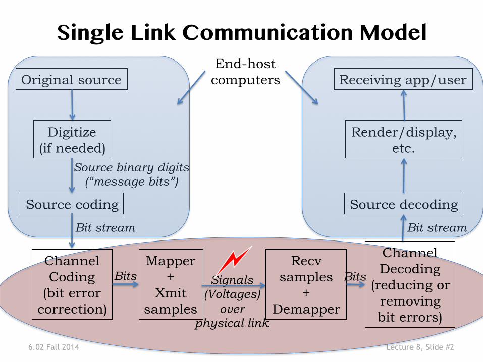
Single Link Communication Model�

Digitize (if needed)

Original source

Source coding

Source binary digits (“message bits”)

Bit stream

Render/display, etc.

Receiving app/user

Source decoding

Bit stream

Channel Coding

(bit error correction)

Recv samples

+ Demapper

Mapper +

Xmit samples

Bits Signals (Voltages)

over physical link

Channel Decoding

(reducing or removing bit errors)

End-host computers

Bits

6.02 Fall 2014 Lecture 8, Slide #3

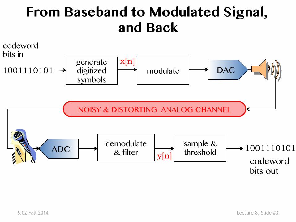
From Baseband to Modulated Signal, and Back �

codeword �bits in �

codeword �bits out �

1001110101 DAC �

ADC �

NOISY & DISTORTING ANALOG CHANNEL�

modulate�

1001110101 demodulate�& filter �

generate�digitized �symbols �

sample & threshold�

x[n]

y[n]

6.02 Fall 2014 Lecture 8, Slide #4

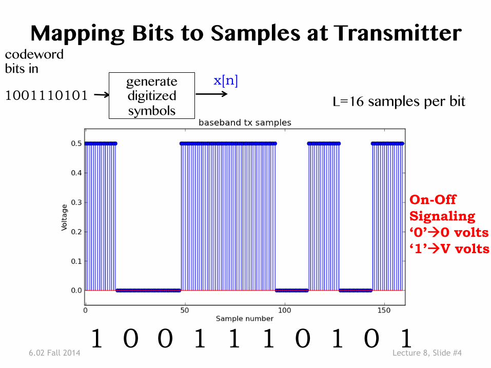
Mapping Bits to Samples at Transmitter �

1 0 0 1 1 1 0 1 0 1

codeword �bits in �

1001110101 generate�digitized �symbols �

x[n]

L=16 samples per bit �

On-Off Signaling ‘0’à0 volts ‘1’àV volts

6.02 Fall 2014 Lecture 8, Slide #5

codeword bits in

1001110101 DAC

ADC

NOISY & DISTORTING ANALOG CHANNEL

modulate

demodulate

generatedigitized symbols

filter

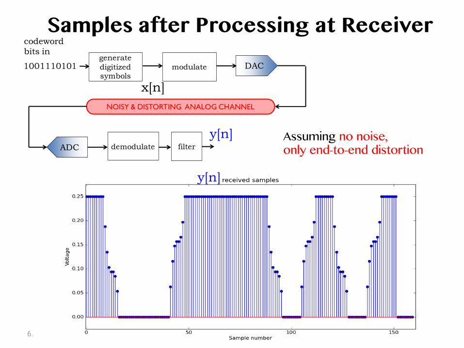
Samples after Processing at Receiver �

x[n]

y[n]

y[n] Assuming no noise, �only end-to-end distortion �

6.02 Fall 2014 Lecture 8, Slide #6

codeword bits in

codeword bits out

1001110101 DAC

ADC

NOISY & DISTORTING ANALOG CHANNEL

modulate

1001110101demodulate& filter

generatedigitized symbols

sample & threshold

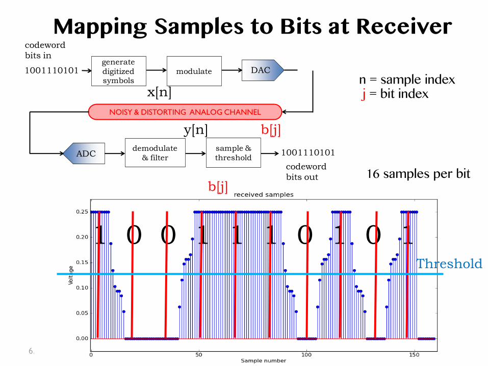
Mapping Samples to Bits at Receiver �

1 0 0 1 1 1 0 1 0 1

16 samples per bit �

x[n]

b[j]

y[n] b[j]

Threshold

n = sample index� j = bit index�

6.02 Fall 2014 Lecture 8, Slide #7

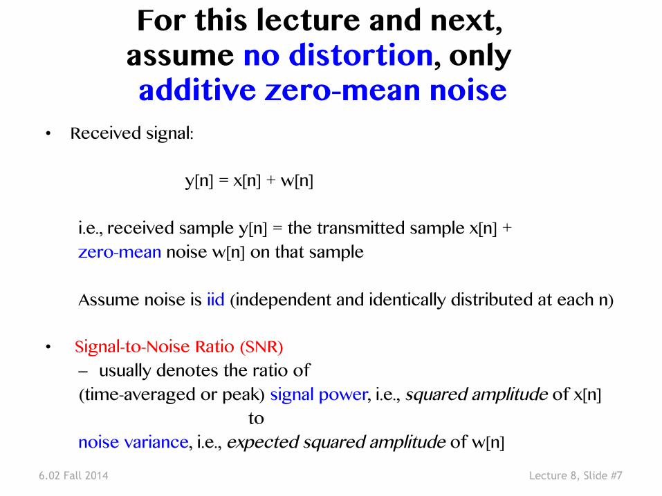
For this lecture and next, �assume no distortion, only �additive zero-mean noise �

•  Received signal: � �

y[n] = x[n] + w[n]��i.e., received sample y[n] = the transmitted sample x[n] + �zero-mean noise w[n] on that sample��Assume noise is iid (independent and identically distributed at each n)��

•  Signal-to-Noise Ratio (SNR)�–  usually denotes the ratio of �(time-averaged or peak) signal power, i.e., squared amplitude of x[n]� to �noise variance, i.e., expected squared amplitude of w[n]�

6.02 Fall 2014 Lecture 8, Slide #8

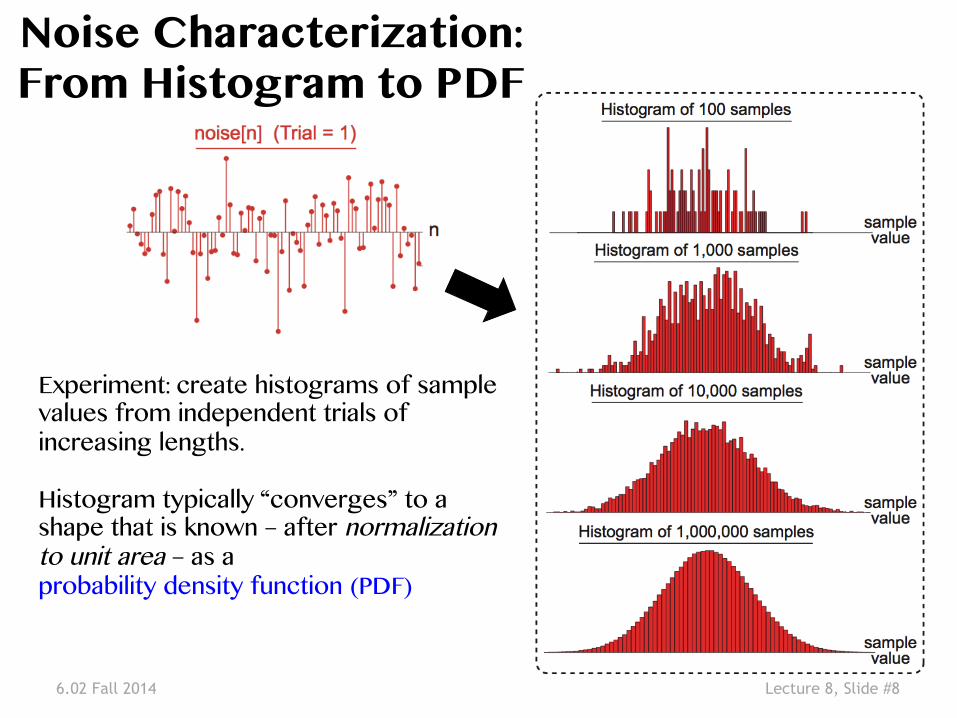
Noise Characterization:�From Histogram to PDF�

Experiment: create histograms of sample values from independent trials of increasing lengths. ��Histogram typically “converges” to a shape that is known – after normalization to unit area – as a �probability density function (PDF)�

6.02 Fall 2014 Lecture 8, Slide #9

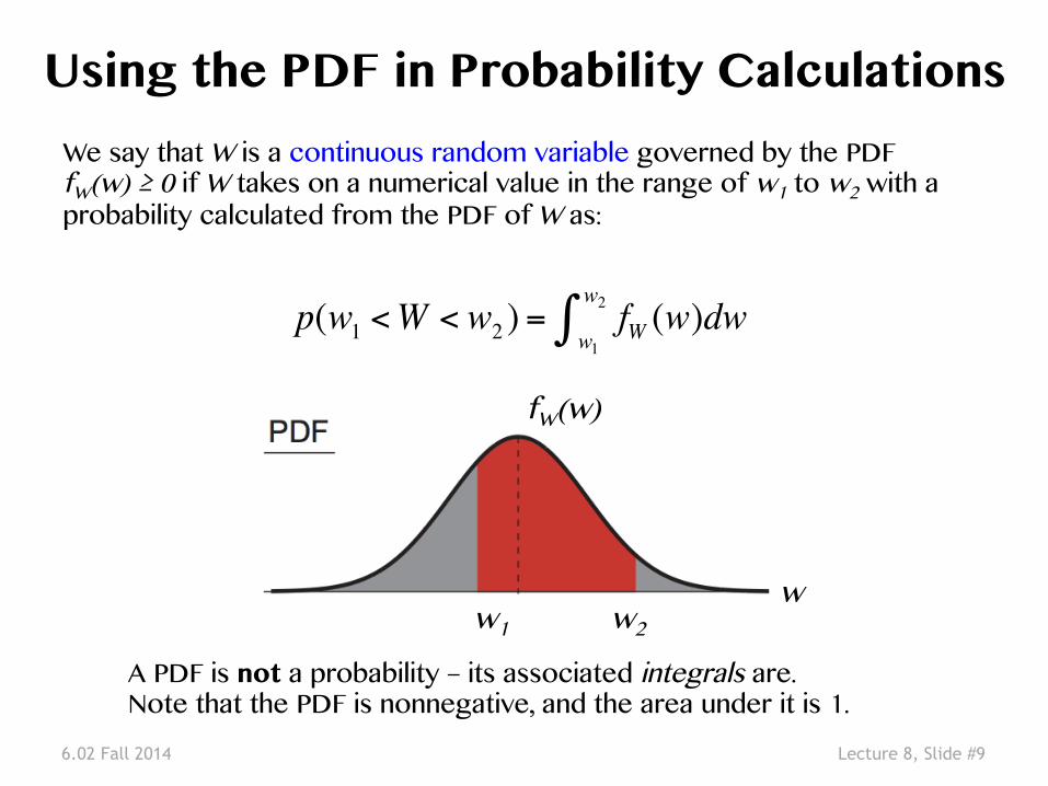
Using the PDF in Probability Calculations�We say that W is a continuous random variable governed by the PDF fW(w) ≥ 0 if W takes on a numerical value in the range of w1 to w2 with a probability calculated from the PDF of W as: �

p(w1 <W < w2 ) = fWw1

w2∫ (w)dw

A PDF is not a probability – its associated integrals are. �Note that the PDF is nonnegative, and the area under it is 1. �

fW(w)

w1 w2 w�

6.02 Fall 2014 Lecture 8, Slide #10

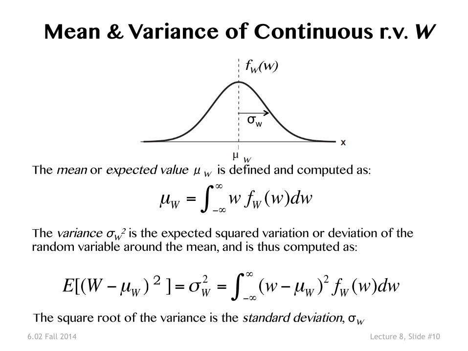
Mean & Variance of Continuous r.v. W�

The mean or expected value μW is defined and computed as: �

The variance σW2 is the expected squared variation or deviation of the

random variable around the mean, and is thus computed as: �

E[(W −µW )2]]=σW2 = (w−µW )

2 fW−∞

∞

∫ (w)dwThe square root of the variance is the standard deviation, σW�

σw

µW = w fW−∞

∞

∫ (w)dw

fW(w)

W�

2

6.02 Fall 2014 Lecture 8, Slide #11

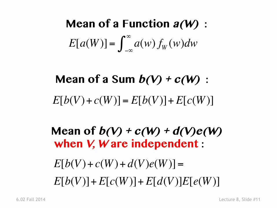
Mean of a Function a(W) :�

E[a(W )]= a(w) fW−∞

∞

∫ (w)dw

E[b(V )+ c(W )+ d(V )e(W )]=E[b(V )]+E[c(W )]+E[d(V )]E[e(W )]

E[b(V )+ c(W )]= E[b(V )]+E[c(W )]

Mean of b(V) + c(W) + d(V)e(W)� when V, W are independent :�

Mean of a Sum b(V) + c(W) :�

6.02 Fall 2014 Lecture 8, Slide #12

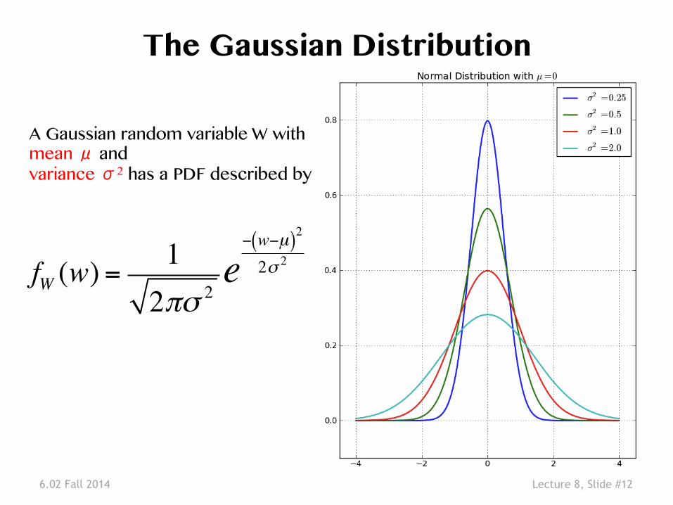
The Gaussian Distribution�

A Gaussian random variable W with �mean μ and �variance σ2 has a PDF described by�

fW (w) =12πσ 2

e− w−µ( )2

2σ 2

6.02 Fall 2014 Lecture 8, Slide #13

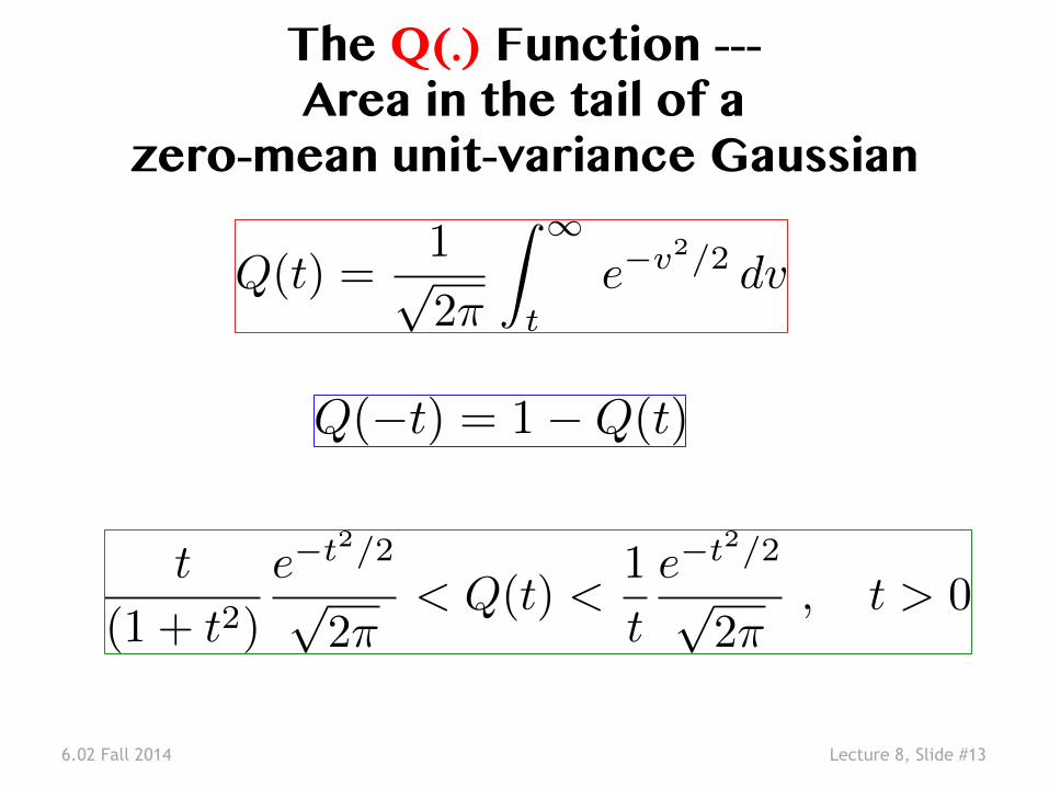
Q(t) =1p2⇡

Z 1

te�v2/2 dv

t

(1 + t2)

e�t2/2

p2⇡

< Q(t) <1

t

e�t2/2

p2⇡

, t > 0

The Q(.) Function --- �Area in the tail of a �

zero-mean unit-variance Gaussian�

Q(�t) = 1�Q(t)

6.02 Fall 2014 Lecture 8, Slide #14

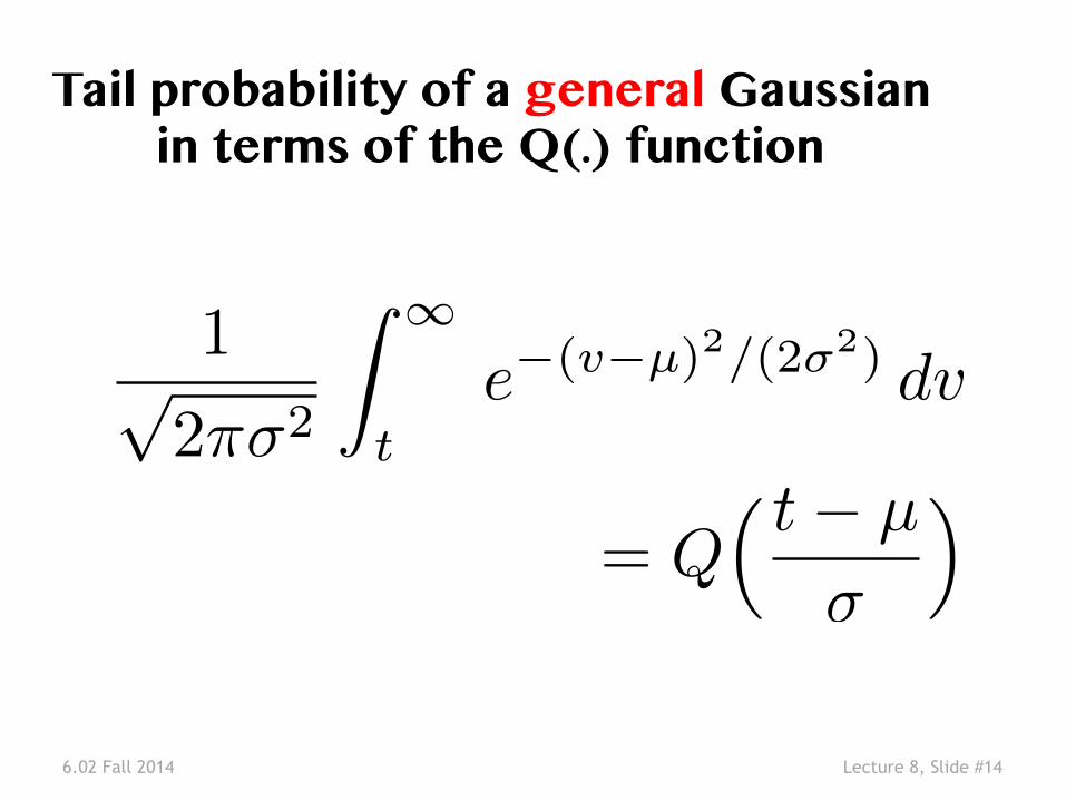
1p2⇡�2

Z 1

te�(v�µ)2/(2�2) dv

= Q⇣ t� µ

�

⌘

Tail probability of a general Gaussian �in terms of the Q(.) function�

6.02 Fall 2014 Lecture 8, Slide #15

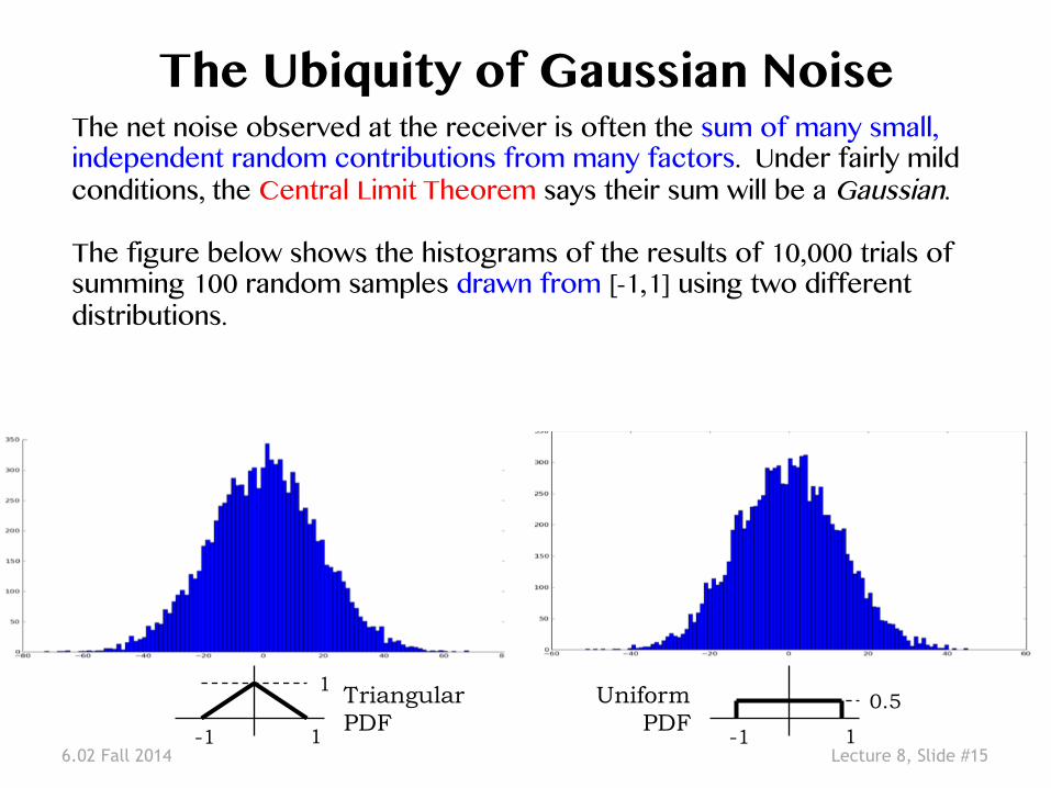
The Ubiquity of Gaussian Noise �The net noise observed at the receiver is often the sum of many small, independent random contributions from many factors. Under fairly mild conditions, the Central Limit Theorem says their sum will be a Gaussian. ��The figure below shows the histograms of the results of 10,000 trials of summing 100 random samples drawn from [-1,1] using two different distributions.�

1 -1

1

1 -1

0.5 Triangular PDF

Uniform PDF

6.02 Fall 2014 Lecture 8, Slide #16

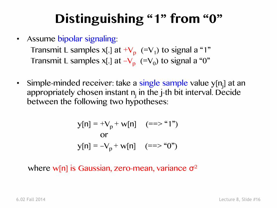
Distinguishing “1” from “0” �•  Assume bipolar signaling: �

Transmit L samples x[.] at +Vp (=V1) to signal a “1”�Transmit L samples x[.] at –Vp (=V0) to signal a “0”�

•  Simple-minded receiver: take a single sample value y[nj] at an appropriately chosen instant nj in the j-th bit interval. Decide between the following two hypotheses: �

y[n] = +Vp + w[n] (==> “1”)� or � y[n] = –Vp + w[n] (==> “0”)�� where w[n] is Gaussian, zero-mean, variance σ2 �

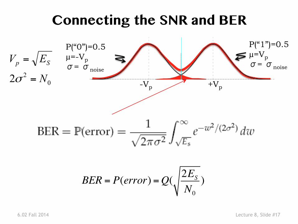
6.02 Fall 2014 Lecture 8, Slide #17

Connecting the SNR and BER �

BER = P(error) =Q( 2ES

N0

)

022 N

EV Sp

=

=

σ

P(“0”)=0.5 µ=-Vp σ= σnoise

P(“1”)=0.5 µ=Vp σ= σnoise

-Vp +Vp

6.02 Fall 2014 Lecture 8, Slide #18

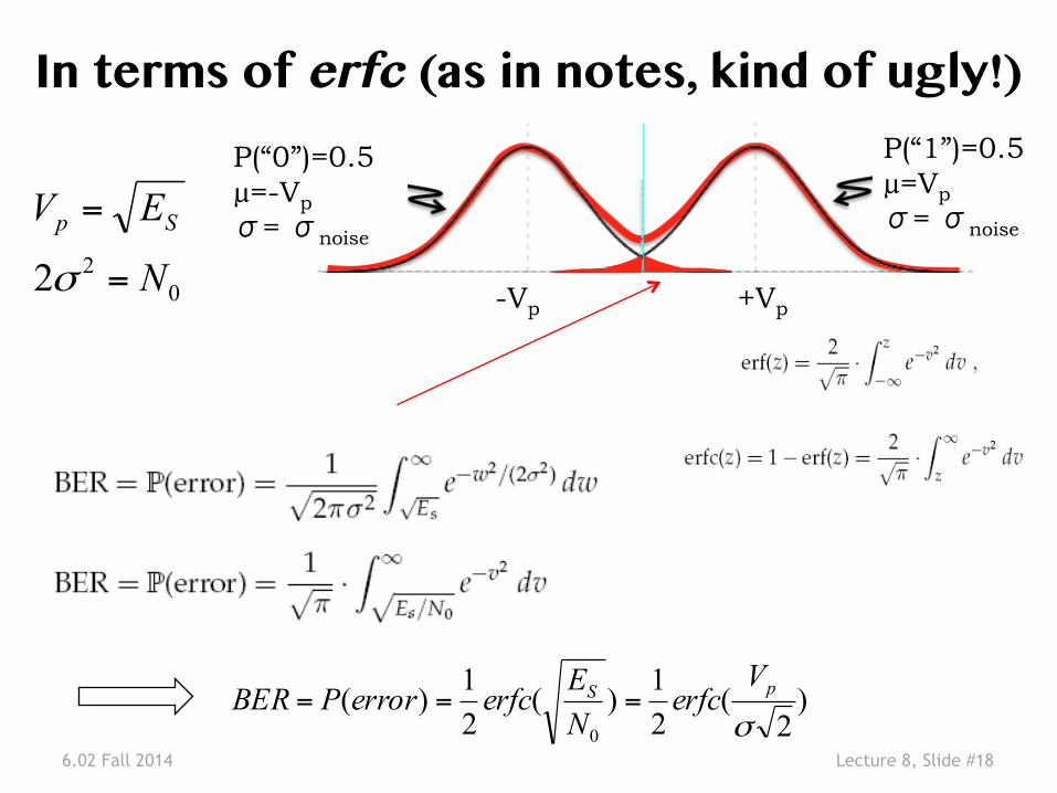
In terms of erfc (as in notes, kind of ugly!)�

)2

(21)(

21)(

0 σpS V

erfcNEerfcerrorPBER ===

022 N

EV Sp

=

=

σ

P(“0”)=0.5 µ=-Vp σ= σnoise

P(“1”)=0.5 µ=Vp σ= σnoise

-Vp +Vp

6.02 Fall 2014 Lecture 8, Slide #19

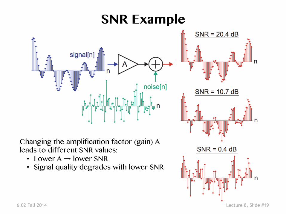
SNR Example �

Changing the amplification factor (gain) A leads to different SNR values: �•  Lower A → lower SNR �•  Signal quality degrades with lower SNR �

6.02 Fall 2014 Lecture 8, Slide #20

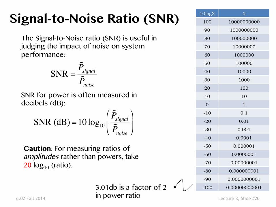
Signal-to-Noise Ratio (SNR)�The Signal-to-Noise ratio (SNR) is useful in judging the impact of noise on system performance: �

SNR =PsignalPnoise

SNR for power is often measured in �decibels (dB): �

SNR (dB) =10 log10

PsignalPnoise

!

"##

$

%&&

10logX X

100 10000000000

90 1000000000

80 100000000

70 10000000

60 1000000

50 100000

40 10000

30 1000

20 100

10 10

0 1

-10 0.1

-20 0.01

-30 0.001

-40 0.0001

-50 0.000001

-60 0.0000001

-70 0.00000001

-80 0.000000001

-90 0.0000000001

-100 0.00000000001 3.01db is a factor of 2 �in power ratio �

Caution: For measuring ratios of �amplitudes rather than powers, take�20 log10 (ratio). �