6 Visibility and Cloud Lidar -...
22
6 Visibility and Cloud Lidar Christian Werner 1 , Jürgen Streicher 1 , Ines Leike 1 , and Christoph Münkel 2 1 Institut für Physik der Atmosphäre, DLR Deutsches Zentrum für Luft- und Raumfahrt e.V. Oberpfaffenhofen, D-82234 Wessling, Germany ([email protected], [email protected], [email protected]) 2 Vaisala GmbH, Schnackenburgallee 41d, D-22525 Hamburg, Germany ([email protected]) 6.1 Introduction Visibility, or visual range, is a property of the atmosphere that has direct significance not just for our pleasure and well-being. Visibility is of decisive importance for all kinds of traffic operations. An uncounted number of victims have been injured or killed because of visibility or, rather, the lack of it. In road traffic a cautious driver can go slowly and stop altogether if, in a snowstorm or in heavy rain or fog, visibility gets worse and worse. This possibility is restricted in boat operations and absent in air traffic. Unlike in situ devices which determine visibility in one point, or fixed installations for the determination of optical transmission between two locations on the ground, lidar allows one to make observations of atmospheric conditions over an extended optical path from one location, fixed or mobile, in any, not just in horizontal direction. Lidar allows quantitative determination of visual range as a function of distance and is thus ideally suited to measure visibility at airports both over the different parts of runways and in the air space above where aircraft safety depends particularly critically on the pilots’ unimpeded view and orientation.
Transcript of 6 Visibility and Cloud Lidar -...
6
Visibility and Cloud Lidar
Christian Werner1, Jürgen Streicher1, Ines Leike1, andChristoph Münkel2
1Institut für Physik der Atmosphäre, DLR Deutsches Zentrum für Luft- undRaumfahrt e.V. Oberpfaffenhofen, D-82234 Wessling, Germany([email protected], [email protected], [email protected])2Vaisala GmbH, Schnackenburgallee 41d, D-22525 Hamburg, Germany([email protected])
6.1 Introduction
Visibility, or visual range, is a property of the atmosphere that has directsignificance not just for our pleasure and well-being. Visibility is ofdecisive importance for all kinds of traffic operations. An uncountednumber of victims have been injured or killed because of visibility or,rather, the lack of it. In road traffic a cautious driver can go slowly andstop altogether if, in a snowstorm or in heavy rain or fog, visibility getsworse and worse. This possibility is restricted in boat operations andabsent in air traffic.
Unlike in situ devices which determine visibility in one point, orfixed installations for the determination of optical transmission betweentwo locations on the ground, lidar allows one to make observations ofatmospheric conditions over an extended optical path from one location,fixed or mobile, in any, not just in horizontal direction.
Lidar allows quantitative determination of visual range as a functionof distance and is thus ideally suited to measure visibility at airportsboth over the different parts of runways and in the air space above whereaircraft safety depends particularly critically on the pilots’ unimpededview and orientation.
166 Christian Werner et al.
6.2 The Notion of Visual Range
Visual range is in this context defined as a local variable of the atmospherethat is directly related to its turbidity: the higher turbidity, the shorter thevisual range.
Visibility is physically limited by two effects: the inability of lightfrom a distant object to reach the eye of the observer due to atmosphericabsorption, and the increase of background light from atmospheric scat-tering between the object and the observer [1]. In other words: an objectcan no longer be seen by the observer if its apparent brightness gets closeto the brightness of the background—exactly how close is a matter ofdefinition as will be shown below.
The magnitude of the former effect is described by the atmosphericabsorption coefficient α(x, λ) which may depend on range x and whichvaries with wavelengthλ. The magnitude of the latter is determined by theatmospheric backscatter coefficient β(x, λ). Visibility also depends onthe position of the sun, on the color of the object, and on other parameters.α and β are related to each other. For molecular scattering they arestrictly proportional, the proportionality factor being α/β = (8π/3) sr.For particle (cloud and aerosol) scattering they are still proportional, butthe factor varies by an order of magnitude with aerosol material, particlesize distribution, moisture, and other aerosol properties.
According to Koschmieder’s theory [2], visual range V is determinedonly by the contrast threshold K an observer needs to distinguish anobject from its background, and by the extinction coefficient α.
Variations in the relation between α and β and all other effectsmentioned are neglected in the simple definition
V (x) = 1
α(x)ln
1
K. (6.1)
The average visual range between two points at distance x1 and x2 isthen given by the obvious relation
V = x2 − x1∫ x2
x1α(ξ)dξ
ln1
K. (6.2)
Clearly, Eq. (6.1) defines a local and Eq. (6.2) an averaged atmosphericproperty.

6 Visibility and Cloud Lidar 167
6.2.1 Normal Visual Range
The convention is that α is taken at λ = 550 nm. At this wavelengthvisual sensitivity is best. Koschmieder [2] sets K = 0.02, the contrastthreshold for a normal-sighted, experienced observer. From Eq. (6.1) wethus obtain the normal visual range, or normal optical range
NOR = 1
αln
1
0.02= 3.912
α. (6.3)
6.2.2 Meteorological Optical Range
For practical purposes a more conservative contrast threshold K = 0.05is assumed, taking into consideration psychological and stress effectsto which an observer such as an aircraft pilot may be exposed, leadingto the shorter so-called meteorological visual range (or meteorologicaloptical range)
MOR = 1
αln
1
0.05= 3
α. (6.4)
The definition of average NOR and average MOR between two pointsis fully analogous to the definition of Eq. (6.2).
6.2.3 Vertical Optical Range
Horizontal stratification, or a marked variation of the extinctioncoefficient with height, is a frequent phenomenon. An observer look-ing up from the ground can see an object up to a height VOR defined, inanalogy to the previous definitions, by the relation
∫ VOR
0α(z)dz = 3. (6.5)
Vertical optical range VOR is, in other words, the height above groundup to which the extinction coefficient α must be integrated to yield thevalue 3; from this height one-twentieth of the light reaches an observeron the ground. Or, more important, 1/20 of the light generated at theground reaches an observer at height VOR (which could be a balloon oraircraft pilot).

168 Christian Werner et al.
6.2.4 Slant Optical Range
Suppose an observer is at a height h above some horizontal plane, whichcan be a runway or, more generally, the ground. Slant optical range(SOR) is the maximum horizontal distance from the point exactly belowhim on the ground to another point on the ground he can see from hisposition at height h. With Pythagoras’ theorem, we have
SOR = h
⎡⎣( 3∫ h
0 α(z)dz
)2
− 1
⎤⎦
1/2
. (6.6)
Slant optical range is thus the projection of a slant line of vision ontothe horizontal plane. Clearly, SOR depends on height h. In most casesSOR decreases as h increases. When h reaches and exceeds VOR, theradicand in Eq. (6.6) gets negative, and SOR vanishes.
6.2.5 Runway Visual Range, Slant Visual Range
For the sake of completeness two more quantities are mentioned here,runway visual range (RVR) and slant visual range (SVR) (as opposed toSOR). These quantities are defined by the International Civil AviationOrganization ICAO [3, 4]. RVR is the maximum distance out to whicha pilot, from a position 5 m above the runway, can recognize either therunway center line or the lights along the runway, defined again by theprojection of the actual optical paths as in Eq. (6.6) onto the runway centerline. In daylight, unless the runway lights are very bright, RVR=MOR.
In a similar way a quantity called slant visual range is defined forpositions h � 5 m. Again, if there are no bright landing fires, thenSVR=SOR in daylight conditions.
6.3 Visibility Measurements with Lidar
Because of its great importance in air traffic, visibility was one of thefirst atmospheric quantities to which the lidar technique was applied [5].As any lidar, visibility lidar also suffered from the problem that twoatmospheric quantities, the absorption coefficient α and the backscattercoefficient β, were to be determined from one measured quantity, thelidar signal.

6 Visibility and Cloud Lidar 169
Attempts to work at different measurement angles [6], use severalwavelengths [7], and utilize reflections from hard targets [8] did notprove applicable. More sophisticated apparatus such as Raman and highspectral resolution lidar (HSRL) systems were not used because of theircomplexity in design and operation. The problem was finally solvedby using essentially the same procedure as that described in Chapter 4,with the simplification that no separate knowledge of the aerosol andmolecule contributions to α and β is necessary, only the total values ofthe respective quantities, or even of total α alone.
The method starts from the familiar lidar equation
P(x, λ) = c�t
2P0
AηO(x)
x2β(x, λ)τ 2(x, λ) (6.7)
withP(x, λ) representing the signal power from distancex at wavelengthλ, P0 the average laser power transmitted during the pulse duration �t ,A and η the receiver area and efficiency, O the laser-beam receiver-field-of-view overlap integral, β the backscatter coefficient, and
τ(x, λ) = exp
[−∫ x
0α(ξ, λ)dξ
](6.8)
the one-way extinction between the lidar and the distance of interest, x.As simple visibility lidars work at one frequency only, we drop λ in therespective quantities and rewrite Eq. (6.7) to yield
P(x) = kO(x)
x2β(x)τ 2(x). (6.9)
We define the quantity
S(x) ≡ P(x)x2
kO(x)= β(x)τ 2(x) (6.10)
and solve the differential equation
∂ ln(S(x))
∂x= 1
β(x)
∂β(x)
∂x− 2α(x) (6.11)
to obtain, with the well-known approximations, the solution
α(x) = S(x)
S(xm)
α(xm)+ 2
∫ xm
x
S(ξ)dξ(6.12)

170 Christian Werner et al.
in a procedure fully analogous to the one described in Chapter 4.It must be noted that in the present application the assumptions andapproximations made in the solution of Eq. (6.11) hold sufficiently well.Equation (6.12) is thus a stable solution of the profile of the extinctioncoefficient α(x). To use it, however, the boundary values of S and α atthe remote end of the lidar range, S(xm) and α(xm), must be known.A data evaluation algorithm stable enough to also work in an automatedregime is the following [9, 10]:
(i) From the signal P(x) of the first measurement of a run, values aredetermined for the minimum and maximum range for which dataevaluation appears meaningful.
(ii) An initial value of α(xm) is chosen that is sufficiently large to leadto reasonably stable integration, but must be within the range ofextinction coefficients that can be determined with the system. Thelower limit of extinction coefficients is given by the signal-to-noiseratio, i.e., by the laser power and the sensitivity of the detector,the upper limit is determined by total extinction and thus, at fixeddistance-bin width, by the number of bins.
(iii) The integration is then carried out within the limits determinedaccording to (i).
(iv) Values of local visibilities are averaged, rejecting values beyondthe limit predetermined in (ii).
(v) The average is compared with the starting value. If the agreementis within 10%, it is considered the final value. If not, the average istaken for the next starting value, and steps (iii) to (v) are repeated. Ifthis was not successful after 10 iterations, the procedure is stoppedwith an error message.
(vi) If the iteration was successful, the resulting value is taken as astarting value for the next run, step (ii).
6.4 Aerosol Distributions
Impaired visibility is always caused by particles in the atmosphere.Particle distributions that frequently affect visibility are convenientlygrouped in categories according to their origin, size, and effects. Particlesize distributions span a wide range of radii r and are generally describedby a modified gamma distribution
n(r) = arε exp(−brγ ) (6.13)

6 Visibility and Cloud Lidar 171
or by sums of such distributions each of which is then called a “mode”[11]. n(r)dr is the number volume density of particles with radii betweenr and r + dr . The constants a, b, ε, and γ are all real and positive. εand γ which describe the steepness of the rise and fall of the distributionare taken as integer and half-integer, respectively. The larger ε and γ ,the steeper and narrower the mode. The radius of particles that are mostabundant, or mode radius, is given by
rc =(
ε
bγ
) 1γ
. (6.14)
The total number density is obtained by integration over all particle radii:
N = a
∫ ∞
0rε exp(−brγ ) dr. (6.15)
When carried out, the integration yields
N = aγ−1b−(a+1)/γ �((a + 1)/γ ). (6.16)
The � function is related to the � function which interpolates thefactorials by the relation �(k) = �(k − 1), with �(0) = �(1) = 1,�(2) = 2, �(3) = 6, etc.
In Table 6.1 nine common types of cloud, fog, and haze have beenlisted along with the parameters that describe particle size distributions if
Table 6.1. Parameters for the particle size distribution for several standard atmosphericconditions
Atmosphericcondition a ε b γ rc (μm) N (m−3)
Advective fogheavy
0.027 3 0.3 1.0 10.0 20 · 106
Advective fogmoderate
0.066 3 0.375 1.0 8.0 20 · 106
Cumulus cloud C1/Radfog heavy
2.373 6 1.5 1.0 4.0 100 · 106
Corona cloud C2 1.085 · 10−2 8 1/24 3.0 4.0 100 · 106
Haze H 4.0 · 105 2 20.0 1.0 0.1 100 · 106
Haze L 4.976 · 106 2 15.119 0.5 0.07 100 · 106
Haze M 16/3 · 105 1 8.943 0.5 0.05 100 · 106
Cloud C3 5.556 8 1/3 3.0 2.0 100 · 106
Radfog moderate 607.5 6 3 1.0 2.0 200 · 106

172 Christian Werner et al.
this distribution is assumed to be monomode. Four of these parameters,e.g., a, b, ε, and γ , can be taken, independently from one another, fromfits to measured distributions. The remaining two are then obtained fromrelations (6.14) and (6.16). In the table, ε, γ , rc, and N were taken asprimary parameters and a and b were calculated.
Scattering angle 180°
rad. mod. rad. heavy adv. mod. adv. heavy
100 1 000 10 000
1.00E-07
1.00E-08
1.00E-09
Visibility, m
Backscattersignal,
arbitraryunits
Scattering angle 30°
rad. mod rad. heavy adv. mod adv. heavy
100 1 000 10 000
1.00E-06
1.00E-07
1.00E-08
Visibility, m
Signalscattered
30° forward,arbitrary
units
Fig. 6.1. Relative magnitude of scattered signal for four types of fog: radiative moderate,radiative heavy, advected moderate, and advected heavy. Whereas backscatter intensities(top) vary by a factor >1.5, 30◦-forward scattering is almost identical (bottom).

6 Visibility and Cloud Lidar 173
Fig. 6.2. Phase functions of spherical particles of different size. Solid line: 1 nmradius (Rayleigh scattering), dotted line: 100 nm, dashed line: 500 nm (Mie scattering).Scattering wavelength is 550 nm, index of refraction 1.55.
Much like the size distributions, the scattering phase functions—or scattering amplitudes—as a function of angle are also different fordifferent weather conditions. For lidar, the scattering angle of relevanceis 180◦. Indeed, backscatter intensities vary by more than a factor of1.5 for different fog conditions (Fig. 6.1, top). It is interesting to notethat at a forward scattering angle of 30◦ these differences nearly vanish(Fig. 6.1, bottom). This is also seen in Fig. 6.2, which gives the scatteringphase functions I for spherical particles of three different sizes. Thesefunctions are normalized such that the integral is unity:∫ 2π
ϕ=0
∫ 1
cosϑ=0I (ϕ, ϑ) d cosϑ dϕ = 1. (6.17)
6.5 Visibility and Multiple Scattering
In dense media, especially in clouds, the backscattered lidar signalmay have undergone more scattering processes than just the near-180◦backscatter process. Multiple scattering (Chapter 3) may stronglyaffect visibility measurements. The extent to which multiple scatteringcontributes to the lidar signal depends on the properties of the particles(size and volume number density, optical depth) and on the geome-try of the lidar: the larger the volume from which light is detected, the
174 Christian Werner et al.
larger the multiple-scattering contribution. The fraction of multiply scat-tered light therefore increases with laser beam divergence, receiver fieldof view, and increasing distance between the lidar and the scatteringvolume.
Lidars are usually characterized by low beam divergence and a narrowreceiver field of view. As large particles scatter light predominantly inthe forward direction (cf. Fig. 6.2), the first scattering process occursmore often than for smaller particles in such a way that the scatteredlight is still within the lidar FOV so that it can directly be backscatteredtowards the receiver. Therefore large particles have the greatest share inmultiple scattering.
Multiple scattering thus results in a reduction of the apparentextinction coefficient and a seemingly longer visual range. The effectis taken into account by appropriate correction terms for dense media.
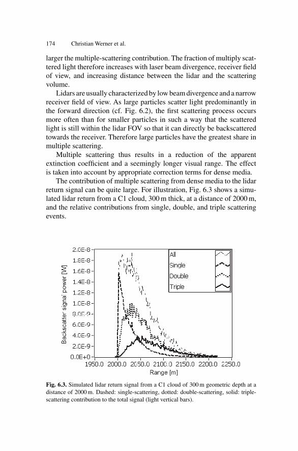
The contribution of multiple scattering from dense media to the lidarreturn signal can be quite large. For illustration, Fig. 6.3 shows a simu-lated lidar return from a C1 cloud, 300 m thick, at a distance of 2000 m,and the relative contributions from single, double, and triple scatteringevents.
Fig. 6.3. Simulated lidar return signal from a C1 cloud of 300 m geometric depth at adistance of 2000 m. Dashed: single-scattering, dotted: double-scattering, solid: triple-scattering contribution to the total signal (light vertical bars).
6 Visibility and Cloud Lidar 175
6.6 Instruments
Visibility lidars are essentially backscatter lidars. Their sophisticationis more in light weight, small volume, reliability, ruggedness, and easeof operation than in the ultimate in power, bandwidth, etc. Visibilitylidar systems are commercially available from several manufacturers.Because they can also be used for other purposes such as cloud heightdetection and aerosol mesasurements, they often come under differentnames.
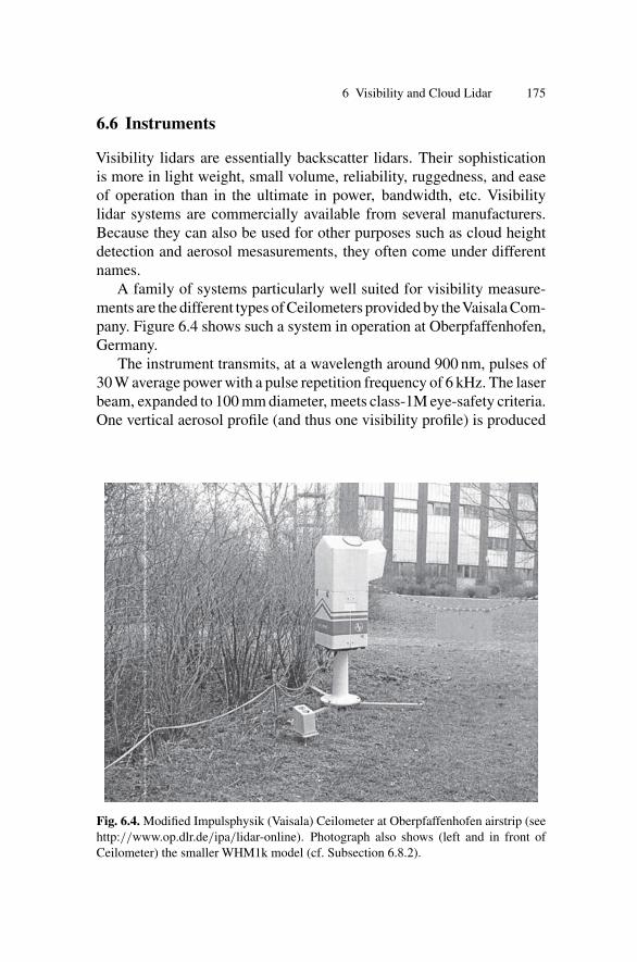
A family of systems particularly well suited for visibility measure-ments are the different types of Ceilometers provided by theVaisala Com-pany. Figure 6.4 shows such a system in operation at Oberpfaffenhofen,Germany.
The instrument transmits, at a wavelength around 900 nm, pulses of30 W average power with a pulse repetition frequency of 6 kHz. The laserbeam, expanded to 100 mm diameter, meets class-1M eye-safety criteria.One vertical aerosol profile (and thus one visibility profile) is produced
Fig. 6.4. Modified Impulsphysik (Vaisala) Ceilometer at Oberpfaffenhofen airstrip (seehttp://www.op.dlr.de/ipa/lidar-online). Photograph also shows (left and in front ofCeilometer) the smaller WHM1k model (cf. Subsection 6.8.2).

176 Christian Werner et al.
every 30 s, although only 10,000 shots per profile are needed. The systemis fully automated and can produce horizontal and slant profiles as well,24 hours a day.
6.7 Applications
Range-resolved recording of the backscattered signal allows the depth-resolved measurement of turbidity and, thus, of the local visibility asdefined in Eq. (6.1), for distances between several meters and a fewkilometers, depending on weather. From that all secondary quantities,whether integrated or not, can be determined. A number of examples ispresented below for illustration.
6.7.1 Meteorological Optical Range (MOR) at Hamburg Airport
During a campaign at the airport of Hamburg, Germany, in 1991 avisibility lidar was installed near the touchdown point. Figure 6.5 shows1.5 hours of lidar data along with the results from a standard trans-missometer. Although the MOR data varied by more than a factor of2.5 during the measurement time, the two sets of data are practicallyidentical with, on average, a slight tendency of the lidar to be lower thanthe transmissometer data (by ≤15%) and thus on the safe side.
Fig. 6.5. Visibility MOR versus time for two sensors, a standard transmissometer and avisibility lidar (airport Hamburg, Germany, 12 January 1992).

6 Visibility and Cloud Lidar 177
6.7.2 Slant Visibility (SOR) at Quickborn
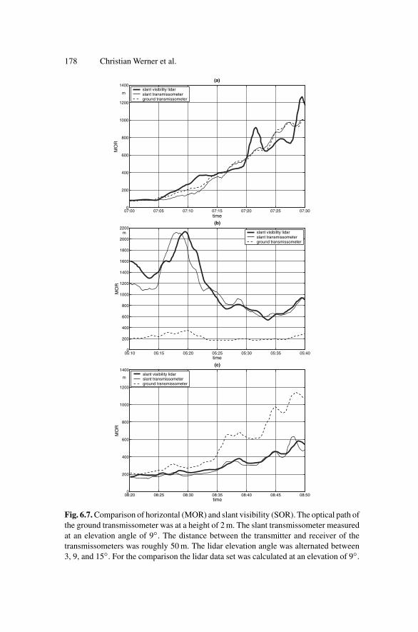
Slant visibility SOR (Eq. 6.6) is particularly important for aircraft landingapproaches in situations of ground fog and lifted fog layers. A campaignto compare MOR and SOR was staged in Quickborn, Germany, from1988 to 1990. Two transmissometers, one slant and one horizontallyoriented, were used between two masts. A visibility lidar measured fromthe same position into several elevation angles. The arrangement of theinstruments is sketched in Fig. 6.6. Figure 6.7 shows results obtained inthree different fog situations. In the event of Fig. 6.7(a) we have relativelyhomogeneous fog which starts to evaporate around 07:05. Slant visibilitySOR increases from about 80 m to more than 1000 m thirty minuteslater and is almost identical to the meteorological optical range MOR.In Fig. 6.7(b) a thin layer of fog on the ground affects the horizontaltransmissometer, but not the slant instruments which yield much highervisual range values. This is the typical situation in which pilots cansee the runway or landing lights but are not allowed to land becausethe ground transmissometer indicates too dense fog on the ground [3].Figure 6.7(c) shows the opposite situation in which the fog has liftedfrom the ground, resulting in good visibility on the ground but poorslant-path visual range [12].
6.7.3 Detection of Clouds
Visibility lidars are very well suited for the detection of clouds down to anoptical thickness that is hard to perceive with the naked eye from below.
ground transmissometer
slant transmissometer
visibility LIDAR
15º
9º
3º
Fig. 6.6. Measurement scenario for comparison of horizontal (MOR) and slant visibility(SOR).
178 Christian Werner et al.
07:00 07:05 07:10 07:15 07:20 07:25 07:300
200
400
600
800
1000
1200
1400
time
RO
M
(a)
slant visibility lidarslant transmissometerground transmissometer
m
05:10 05:15 05:20 05:25 05:30 05:35 05:400
200
400
600
800
1000
1200
1400
1600
1800
2000
2200
time
RO
M
(b)
slant visibility lidarslant transmissometerground transmissometer
m
08:20 08:25 08:30 08:35 08:40 08:45 08:500
200
400
600
800
1000
1200
1400
time
RO
M
(c)
slant visibility lidarslant transmissometerground transmissometer
m
Fig. 6.7. Comparison of horizontal (MOR) and slant visibility (SOR). The optical path ofthe ground transmissometer was at a height of 2 m. The slant transmissometer measuredat an elevation angle of 9◦. The distance between the transmitter and receiver of thetransmissometers was roughly 50 m. The lidar elevation angle was alternated between3, 9, and 15◦. For the comparison the lidar data set was calculated at an elevation of 9◦.

6 Visibility and Cloud Lidar 179
Fig. 6.8. Screenshot of vertical fog profile measurements from 8 May 2001, 08:42, to9 May 2001, 08:41. The plot at right is the actual lidar signal.
Figure 6.8 shows a color-coded intensity plot of the optical density asa function of altitude and time, in a sequence of one profile every 30 s.The red vertical bar is the actual time (08:41 in this case), the data tothe right of the red line are the results of the previous day. The seamlesstransition to the profiles 24 hours before is purely accidental. The actualheight profile of the lidar signal is shown on the right. We note thepresence of fog and of clouds most of the time, at an altitude that variesbetween less than 100 m in the early morning and about 1200 m around20:00 hours. Although the measurement range of the system is 3500 m,the signal gets extinct after 250 m because of the dense fog layer whichstarts at 160 m altitude.
6.7.4 Cloud Ceiling
Figure 6.9 gives an example of two cloud layers appearing in the profilefrom a standard commercial ceilometer, illustrating the ability to detecthigh cirrus clouds.
The standard reporting frequency of ceilometers in use at airports isone set of data every 15 s. An automatic cloud algorithm investigates theshape of the backscatter profile, discards maxima originating from signalnoise or falling precipitation, and generates a data message with cloud

180 Christian Werner et al.
Fig. 6.9. Ceilometer backscatter signal from boundary layer aerosol and two cloud layerswith base heights of 5700 m and 9600 m. Profile taken with a Vaisala LD-40 Ceilometeron 13 May 2001, 22:15:16 – 22:16:46, averaged over 382,752 pulses.
0
20
40
60
80
100
120
140
160
180
200Grayscale−coded ceilometer backscatter intensity in 10−8 m−1 sr−1
Time on 10.05.2003
Hei
ght i
n m
00:00 03:00 06:00 09:00 12:000
100
200
300
400
500
600
700
800
900
1000
Fig. 6.10. Grayscale-coded intensity plot of range-corrected ceilometer backscatterprofiles (Hamburg, Germany, 10 May 2003).

6 Visibility and Cloud Lidar 181
base heights and instrument status information. Additional parametersreported include vertical visibility and the amount of precipitation.
Even in clear-atmosphere situations like the one prevailing inFig. 6.9 there is enough backscatter signal detected from altitudes up to1000 m to estimate the aerosol concentration in the planetary boundarylayer.
6.7.5 Mass Concentration Measurements
When the visual range exceeds 2000 m, a standard ceilometer designedto detect cloud bases still receives a considerable amount of backscattersignal from boundary-layer aerosol. The grayscale-coded intensity plotin Fig. 6.10 gives an example.
Comparisons with in situ sensors measuring dust concentration val-ues (PM10 and PM2.5) show a good correlation between ceilometersignal and dust concentration measured in the corresponding altitude[13]. Figure 6.11 shows this relationship using an empirically derived
Fig. 6.11. Dust concentration derived from ceilometer backscatter between 0 and 30 maltitude and PM10 concentration between 0 and 20 m height (Hannover, Germany, 24March to 12 April 2002).

182 Christian Werner et al.
linear dependency between ceilometer backscatter and PM10 massconcentration.
6.8 Recent Developments
6.8.1 Intelligent Taillight: Adaptation of Brightness Using theLidar Technique
Although in many regions road traffic density has increased dramatically,the rate of accidents has generally decreased. A good deal of this trendis due to the development of equipment that increases traffic safety. Thecontinuation of this process thus deserves particular attention [14, 15].
The perceptibility of automotive lighting and light signals under poorvisibility conditions is one important field in this context. The problem isnot just precipitation and fog. On a wet road spray whirled up by tires alsoaffects visibility quite strongly. Depending on the amount of moistureon the road and on driving speed, this spray is dragged like a flag morethan 20 m behind the vehicle. A measuring principle based on spot-likescanning of only a small volume is not suited for the initialization ofany countermeasures. Rather, a method is needed that can measure theturbidity in an extended measuring volume. The exact size of that volumemay have to be adapted to the vehicle’s speed.
To help improve the visibility of vehicle rear lights to the driverof the vehicle behind, a system is under development for installa-tion in automobile taillights that must be able to detect the followingparameters:
• visibility reduction by rain, snow, fog or tire spray,• distance of the following car and• speed of the following car.
The sensor data are then transferred to a unit called rear light con-troller (RLC) in which these and other automotive data are linked toa weather model to generate control signals that regulate the bright-ness of the lamps. The complete lidar system consists of a transmitter(a laser diode and an optical lens), a receiver (an optical lens and anavalanche photodiode) and a data acquisition system (a digitizer andmicrocomputer). The whole system including the electronic lamp bright-ness regulator is housed in a box the size of a car radio. The first prototypeis shown in Fig. 6.12 built into the rear part of an automobile. The
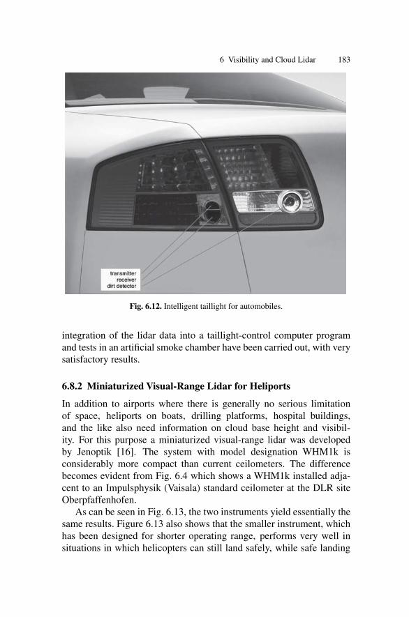
6 Visibility and Cloud Lidar 183
Fig. 6.12. Intelligent taillight for automobiles.
integration of the lidar data into a taillight-control computer programand tests in an artificial smoke chamber have been carried out, with verysatisfactory results.
6.8.2 Miniaturized Visual-Range Lidar for Heliports
In addition to airports where there is generally no serious limitationof space, heliports on boats, drilling platforms, hospital buildings,and the like also need information on cloud base height and visibil-ity. For this purpose a miniaturized visual-range lidar was developedby Jenoptik [16]. The system with model designation WHM1k isconsiderably more compact than current ceilometers. The differencebecomes evident from Fig. 6.4 which shows a WHM1k installed adja-cent to an Impulsphysik (Vaisala) standard ceilometer at the DLR siteOberpfaffenhofen.
As can be seen in Fig. 6.13, the two instruments yield essentially thesame results. Figure 6.13 also shows that the smaller instrument, whichhas been designed for shorter operating range, performs very well insituations in which helicopters can still land safely, while safe landing

184 Christian Werner et al.
Fig. 6.13. WHM1k optical-density plot from 8 January 2004.
of an airplane would be a considerable challenge. It clearly indicates,however, visibility conditions too poor for a landing approach of thehelicopter as well, as is the case between 01:34 and 10:10 in the graph.Figure 6.13 shows the fog recording from 8 January 2004.
Both devices clearly ‘see’ground fog with patches of varying densityfrom midnight to approximately 11:00. During that time the inversionand cloud detection algorithm registers alarm conditions from the dataof both systems: cloud altitude is below 150 m, and vertical visibility isbelow 800 m. The numerical differences in vertical visibility between theWHM1k (about 100 m) and the ceilometer (about 300 m) are caused bythe AC-coupled detection unit of the WHM1k sensor. The smooth signalfrom the homogeneous fog layer is interpreted as a DC background andcut off by the 1-kHz high-pass filter of the receiver electronics.
6 Visibility and Cloud Lidar 185
From Fig. 6.13 it can also be seen that the fog layer starts to rise atapproximately 11:00 hours. The ceilometer still measures some impair-ment of local visibility, but as this happens at altitudes above 150 m,VFR (i.e., visual flight rule) conditions still prevail. The WHM1k cloud-altitude algorithm follows the rise of the cloud, which seems to becomethinner in the WHM1k density plot (top left), but not in the ceilometerplot (top right). This effect occurs only at night. The reason is the factthat the sensitivity control of the APD current is carried out using thebackground light information. This also needs to be improved. We thussee that downscaling a well-tested, trustworthy, and reliable system stillconstitutes a technological challenge.
6.9 Summary
In summary it can be stated that visibility lidar is an accepted technologywherever impaired vision must be detected to impose speed limits to roador takeoff and landing restrictions to air traffic. Visibility lidars known asceilometers have reached a degree of maturity to work 24 hours a day inthe required fully-automated, hands-off operation mode. The develop-ment of much smaller systems for use under restricted space conditionsand of systems small and cheap enough to be used as a truck and caraccessory is in progress, with good chances to reach full commercialavailability soon.
References
[1] W.E.K. Middleton: Vision through the Atmosphere (University of Toronto Press,Toronto 1952)
[2] H. Koschmieder: Beiträge zur Physik der freien Atmosphäre 12, 33 (1924)[3] ICAO (International CivilAviation Organization): Manual of RunwayVisual Range
Observing and Reporting Practices (Doc 9328-AN/908), Toronto, 2000[4] World Meteorological Organization: Guide to Meteorological Instruments and
Methods of Observation. Sixth Edition, p. 1.9.1, Geneva, 1996[5] R.T.H. Collis, W. Viezee, E.E. Uthe, et al.: Visibility measurements for aircraft
landing operations. AFCRL Report – 70-0598 (1970) – also FAA document DoT-FA70WAI-178
[6] G.J. Kunz: Appl. Opt. 26, 794 (1987)[7] J.F. Potter: Appl. Opt. 26, 1250 (1987)[8] R.B. Smith, A.I. Carswell: Appl. Opt. 25, 398 (1986)[9] German Patent DE 196 42 967 C1 (1998)
[10] VDI Guideline VDI 3786 Part 15: Visual-range lidar (Beuth Verlag, Berlin 2004)

186 Christian Werner et al.
[11] D. Deirmendjian: Electromagnetic Scattering on Spherical Polydispersions(Elsevier, New York 1969)
[12] J. Streicher, C. Münkel, H. Borchardt: J. Atmos. Oceanic Tech. 10, 718 (1993)[13] C. Münkel, S. Emeis, W.J. Müller, et al.: Proc. SPIE 5235, 486 (2004)[14] J. Streicher, C. Werner, J. Apitz, et al.: Europto Proceedings 4167, 252 (2001)[15] R. Grüner, J. Schubert: Proc. SPIE 5240, 42 (2004)[16] J. Streicher, C. Werner, W. Dittel: Proc. SPIE 5240, 31 (2004)