6 Travel Demand and Forecasting - Rocky Mountain...

Rocky Mountain Rail Authority

High‐Speed Rail Feasibility Study

Business Plan

TEMS, Inc. / Quandel Consultants, LLC / GBSM, Inc. March 2010 6‐1

6 Travel Demand and Forecasting

This chapter describes the major steps taken to develop the travel demand model for the RMRA

high‐speed rail system. The demand model predicts public responses in the RMRA study region to

various rail service characteristics including train frequency, travel time, and fares.

The creation of the travel demand model for the RMRA high‐speed rail study required the

delineation of the study area and definition of a zone system; collection of data including stated

preference survey data, socioeconomic data and origin‐destination data; and development of

transportation networks for the competing intercity modes of travel (auto, air, bus, and rail). (See

Appendix C for more details of zones and demand forecast models)

6.1 The Zone System

An early step in developing the forecasting tool was developing the RMRA zone system to provide a

precise definition of travel between the origins and destinations in the corridor. The zone system

provides a reasonable representation of the market area in which travel would be served by the

high‐speed rail system. It covers the whole state of Colorado, as well as portions of the adjoining

states of Wyoming, New Mexico, Utah and Kansas.

Exhibit 6‐1: RMRA Zone System



Business Plan


The zone system of RMRA, as shown in Exhibit 6‐1, is a combination of Colorado Metropolitan

Planning Organization (MPO) zones for the urban areas, while for rural areas, it is predominantly

county based. For both the MPO and county‐based zones base year estimates were developed for

population, income, and employment. These forecasts were compatible with MPOs’ data, Colorado

State Demography Office (Colorado SDO) and the Bureau of Economic Analysis (BEA). Zones are

defined relative firstly to the rail network and secondly to the highway network. As zones move

outward from populated centers, their size transitions from small to larger. For the purpose of

describing the air traffic, some specific zones are designated for the airports. For example, Denver

International Airport (DIA), the largest airport within the study area, has its own zone.

The networks and zone systems developed for the RMRA High‐Speed Rail Feasibility Study were

enhanced with finer zone detail in urban areas. These finer zones were based on the Traffic Analysis

Zones (TAZ) for the five Colorado MPOs that are part of the study area. The whole zone system

contains 194 zones within the study area boundaries and 178 within Colorado. 82 zones are based on

Denver Regional Council of Governments (DRCORG) TAZ, 8 zones from North Front Range MPO

TAZ, 8 zones from Grand Valley MPO TAZ, 5 zones from Pikes Peak MPO TAZ and 7 zones from

Pueblo Area Council of Governments TAZ. Exhibit 6‐1 shows the whole zone system (with the

internal and external zones), while Exhibit 6‐2 shows the zone system in Colorado only*. Exhibit 6‐3

shows the zone system used for Denver area, which is an aggregation of the TAZ system of DRCOG.

Exhibit 6‐2: Colorado Zone System Showing MPOs

* For different networks either ”Full” or “Colorado only” zone systems were used in the RMRA study



Business Plan


Exhibit 6‐3: DRCOG – Denver TAZ Based Zones

The zone system has been incorporated into the COMPASS™ model structure (see Exhibit 6‐4),

which includes four databases:

Stated Preference Data

Socioeconomic Database

Each of these databases is described in the following sections of this chapter.

Origin‐Destination Data

Network Data



Business Plan


Exhibit 6‐4: COMPASS™ Model Structure

These databases are used to calibrate the model, and identify the following demand models:

Total Demand Model (Natural Growth Impact)

Induced Demand Model (Induced Mobility)

Modal Split Model (Market Share by Mode)

6.2 Stated Preference Survey

Stated preference surveys provide critical insight into travel markets and travel behavior. To better

understand the different trip modes, purposes, and seasonal patterns, stated preference surveys

were conducted in different places and in different seasons to capture a representative sample for

each type of traveler.

The purpose of conducting the surveys was to collect specific attitudinal data by interviewing

travelers within the study region. The travelers were asked to identify how they value travel time

and frequencies associated with particular modes of transportation. These values were then

combined with other collected trip data and incorporated into the calibration process for the travel

demand model. The calibration process adapts the model to the specific characteristics of the travel

market within the RMRA study region.



Business Plan


6.2.1 Survey Methodology

Travel options in a stated preference survey enable respondents to consider the trade‐offs among

desirable travel attributes, such as time, comfort, cost, speed, and accessibility without regard to

travel mode. Trade‐offs included a range of service options that were presented in such a way as to

induce the individuals to respond realistically without specifying a mode of travel. More

specifically, stated preference surveys ask travelers to choose between a hypothetical cost and

another value, such as travel time or service frequency. The choice the traveler makes demonstrates

his or her preference between cost, time and other travel aspects of the rail mode. In addition to

estimating the value of time and frequency, the stated preference surveys can also help to get the

information that can be used to determine the trip purposes and trip modes and to evaluate origin

destination flow.

The stated preference surveys for this study were conducted using a stratified or quota group

sampling approach. The information collected from the respondents for a specific quota sampling

category was then expanded to the overall quota sample population based on a mode and purpose

basis (see Exhibit 6‐5). Stratified or quota surveys, which are now widely used in commercial,

political and industrial surveying, have the advantage of being relatively inexpensive to implement

while providing expanded coverage and more representative results than a simple random survey.

Exhibit 6‐5: Modes and Trip Purpose Basis of Stated Preference

The study team developed surveys for each travel mode and purpose. Each survey collected

information on an individual travel profile, origin and destination, trip purposes, demographics, as

well as Stated Preference questions on values of time (VOT), values of service frequency (VOF),

value of interchange and value of reliability. A minimum sample from each travel market segment

(by mode and trip purpose) was required to ensure statistical confidence. Using the Central Limit

Bus

SocialTouris

m Comm

uter

Auto Rail Air

Social

Tourism

Commuter

Business

SocialTouris

m Comm

uter

SocialTouris

m Comm

uter

Social Touris

m Comm

uter



Business Plan


Theorem1, it was determined that a minimum sample size of 20 to 40 participants ensures the

statistical validity for each quota sample. For this study’s stated preference surveys, most of desired

quota targets were set at 80 or more interviews. An example of the sample survey form is shown in

Appendix D.

6.2.2 Survey Implementation

Two sets of stated preference surveys were conducted at various locations within the study region in

a manner designed to reach a broad sample of the potential users of an intercity passenger rail

system. The first one was done in Fall 2008 and the second was done in Winter 2009. The fall survey

was primarily targeted at the Colorado resident and non‐seasonal tourism and the winter survey

was targeted at the resorts trips and employee trip making. Exhibit 6‐6 shows the locations of these

surveys.

Exhibit 6‐6: Locations of Surveys

1 The Central Limit Theorem states that the sampling distribution of the mean of any distribution with mean µ and variance σ2

approaches a normal distribution with mean µ and variance σ2/N as N the sample size increases. Spiegel, M.R., Theory and

Problems of Probability and Statistics, NY McGraw Hill, pp. 112-113, 1992



Business Plan


Approximately 3,659 surveys were completed. The Exhibit 6‐7 shows the target number of each sub‐

group by trip mode and trip purpose and the actual number of surveys received. Based on this

Exhibit, most of groups attained their target values; ensuring the integrity of the sample frame. The

surveys were conducted by using random walk face‐to‐face interview techniques. The surveys

captured data from a broad mix of business travelers, tourists and resident leisure travelers.

Exhibit 6‐7: The Target /Actual Number of Surveys

Business Commuter Social Tourist Total

Rail 0 / 9 0 / 2 80 / 68 160 / 140 240 / 219

Air Access 80 / 391 80 / 13 80 / 433 80 / 480 320 / 1317

Bus 80 / 47 160 / 180 160 / 119 80 / 101 480 / 447

Auto 160 / 260 160 / 171 80 / 489 160 / 746 560 / 1666

Total 320 / 707 400 / 366 400 / 1109 480 / 1467 1600 / 3659

Air mode surveys were conducted at DIA both in winter and fall. The fall surveys targeted

passengers flying directly to or from DIA and excluded connecting passengers, while the winter

surveys focused on intrastate flights, such as to and from Colorado Springs, Aspen, and captured

mostly connecting passengers.

The auto mode surveys were conducted at the Division of Motor Vehicles of Colorado Department

of Revenue and its offices in the cities of Parker (Full Service Office, 17737 Cottonwood Drive),

Colorado Springs (Full service office, Austin Bluffs Pkwy), Pueblo (Full service office, Abriendo

Ave), Grand Junction (Full Service office, 6th St.) and Glenwood Springs (Full service office,

Glenwood Springs Mall). In winter, surveys were carried out at the resort areas of Vail,

Breckenridge, and Central City.

Rail mode surveys were conducted at the Amtrak stations before passengers boarding on trains. The

surveyed stations included Denver Union Station, Grand Junction, and Glenwood Springs.

Bus mode surveys were conducted at stations of RTD, Greyhound and Front Range Express (FREX),

which cover the both long and short distance bus trips.



Business Plan


6.2.3 Survey Demographic Characteristics

It was found in the survey that there were distinctly different travel and demographic differences on

a modal basis. For example, among air passengers, about 30 percent are business trips, while only 4

percent of rail trips (Amtrak) are business trips, as shown in Exhibit 6‐8.

Exhibit 6‐8: Trip Purposes by Modes

Air Trips by Purpose

Business30%

Commuter1%

Recreation / Vacation

33%

Visit with Family / Friends

30%

Other 5%

Travel to / from School

1%

Auto Trips by Purpose

Travel to / from School

2%

Other16%

Business 20%

Commuter13%


23%

Visit with Family / Friends

26%

Rail Trips by Purpose

Commuter

1% Business

4%

Travel to /

from School

1%

Other

3%

Recreation /

Vacation

64%Visit with

Family /

Friends

29%

Percent of Intercity Bus Trips by Purpose

Business 4%


10%

Travel to /

from School

3%

Visit with Family /

Friends

35%

Commuter 25%

Other

23%

Intercity Bus Trips by Purpose

Business 4%


10%

Travel to /

from School

3%

Visit with Family /

Friends

35%

Commuter 25%

Other

23%



Business Plan


Exhibit 6‐9: Household Income by Modes

Air passengers generally have the highest income, rail and auto passengers have the medium

income while bus passengers have the lowest income (See Exhibit 6‐9).

A comparison of the results of the stated preference survey household income data with the

statewide data shows that the income distributions by mode are representative of statewide data

(see Exhibit 6‐10). A statistical T test shows the income distribution of the modal data from the

survey (when combined appropriately by being weighted) is equivalent to the statewide distribution.

This means that the database will be representative of statewide value of time. As a result, there was

no need of further adjustments to make the data an effective representation of statewide values for

VOT, VOF, etc.

Household Income of Air Travelers

14%

18%

23%

45%

Less than $45,000$45,000 - 64,999

$65,000 - 99,999$100,000 or more

Household Income of Auto Travelers

22%

40%

21%

17%Less than $45,000$45,000 - 64,999

$65,000 - 99,999$100,000 or more

Household Income of Intercity Bus Travelers

67%

18%

11%

4%

Less than $45,000$45,000 - 64,999

$65,000 - 99,999$100,000 or more

Household Income of Rail Respondents

22% 34%

20% 24%

Less than $45,000$45,000 - 64,999

$65,000 - 99,999$100,000 or more



Business Plan


Exhibit 6‐10: Comparison of Household Income Distribution

Source: TEMS, Inc. and U.S. Census Bureau, 2005‐2007 American Community Survey

6.2.4 Value of Time and Value of Frequency by Trip Purpose and Mode

Exhibit 6‐11 and Exhibit 6‐12 illustrate the different values of time and values of frequency

expressed by four trip purposes in the various modes.

Exhibit 6‐11: Value of Time by Trip Purpose and Mode ($/hour)

Trip Purposes Mode

Business Commuter Tourism Social

Bus 13.20 10.92 11.39 11.60

Rail 16.07 17.50 17.65 15.92

Auto 18.91 18.95 18.86 17.69

Air 48.69 35.73 33.34 34.69

0.00

5.00

10.00

15.00

20.00

25.00

Less than$10,000

$10,000 to$14,999

$15,000 to$24,999

$25,000 to$34,999

$35,000 to$49,999

$50,000 to$74,999

$75,000 to$99,999

$100,000 to$149,999

$150,000 to$199,999

$200,000 ormore

Range of Household Income (2007$)

In P

erce

nt

Weighted Average of Survey Results Statewide



Business Plan


Exhibit 6‐12: Value of Frequency by Trip Purpose and Mode ($/hour)

Trip Purposes Mode

Business Commuter Tourism Social

Bus 6.79 6.27 7.08 6.22

Rail 12.88 10.00 14.65 13.31

Air 18.13 21.10 16.75 18.29

As shown in Exhibit 6‐11 and Exhibit 6‐12:

The value of time and value of frequency of air mode are higher than those of other modes.

The bus mode has the lowest value of time and value of frequency.

The business traveler and commuters usually place higher values on travel time.

Compared with other trip purposes, tourism and social trips have lower VOT and VOF.

6.2.5 Comparison with Other Studies

Exhibit 6‐13: Comparison of VOT ($/Hour)

Exhibit 6‐13 provides a comparison of values of time by mode and trip purpose for this study with

the values generated for the MWRRI and the Cleveland Hub Study. It is noted that values of time of

business trips for this study are lower than those for the MWRRI and Cleveland Hub Study, but the

pattern are similar: value of time for air mode is the highest followed by auto and rail while the

values for bus are the lowest. Business trips have higher VOT, while non‐business trips have lower

VOT.

Colorado Midwest Regional Rail

Initiative Cleveland Hub

Mode

Business Non-

Business Business Non-Business Business Non-Business

Air 48.69 34.59 55.12 27.56 79 31

Auto 18.91 18.50 22.58 15.86 26 19

Bus 13.20 11.30 N/A 9.66 16 11

Rail 16.07 17.02 25.22 18.61 33 16



Business Plan


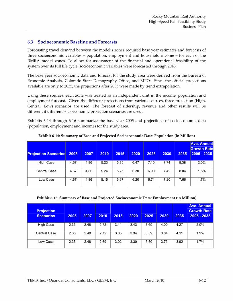
6.3 Socioeconomic Baseline and Forecasts

Forecasting travel demand between the model’s zones required base year estimates and forecasts of

three socioeconomic variables – population, employment and household income – for each of the

RMRA model zones. To allow for assessment of the financial and operational feasibility of the

system over its full life cycle, socioeconomic variables were forecasted through 2045.

The base year socioeconomic data and forecast for the study area were derived from the Bureau of

Economic Analysis, Colorado State Demography Office, and MPOs. Since the official projections

available are only to 2035, the projections after 2035 were made by trend extrapolation.

Using these sources, each zone was treated as an independent unit in the income, population and

employment forecast. Given the different projections from various sources, three projection (High,

Central, Low) scenarios are used. The forecast of ridership, revenue and other results will be

different if different socioeconomic projection scenarios are used.

Exhibits 6‐14 through 6‐16 summarize the base year 2005 and projections of socioeconomic data

(population, employment and income) for the study area.

Exhibit 6‐14: Summary of Base and Projected Socioeconomic Data: Population (in Million)

Projection Scenarios 2005 2007 2010 2015 2020 2025 2030 2035

Ave. Annual Growth Rate 2005 - 2035

High Case 4.67 4.86 5.23 5.85 6.47 7.10 7.74 8.38 2.0%

Central Case 4.67 4.86 5.24 5.75 6.30 6.90 7.42 8.04 1.8%

Low Case 4.67 4.86 5.15 5.67 6.20 6.71 7.20 7.66 1.7%

Exhibit 6‐15: Summary of Base and Projected Socioeconomic Data: Employment (in Million)

Projection Scenarios 2005 2007 2010 2015 2020 2025 2030 2035


High Case 2.35 2.48 2.72 3.11 3.43 3.69 4.00 4.27 2.0%

Central Case 2.35 2.48 2.72 3.05 3.34 3.59 3.84 4.11 1.9%

Low Case 2.35 2.48 2.69 3.02 3.30 3.50 3.73 3.92 1.7%



Business Plan


4.5

5

5.5

6

6.5

7

7.5

8

8.5

9

2000 2005 2010 2015 2020 2025 2030 2035 2040

Mill

ions

High Case

Central Case

Low Case

Exhibit 6‐16: Summary of Base and Projected Socioeconomic Data: Average Household Income

(in Thousand $2007)

Projection

Scenarios 2007 2010 2015 2020 2025 2030 2035


High Case 68.483 73.87 80.03 84.31 87.59 91.31 95.04 1.2%

Central Case 68.483 72.45 78.17 81.25 84.36 87.39 90.55 1.0%

Low Case 68.483 71.46 72.48 74.92 77.23 79.42 81.58 0.6%

Note: future data adjusted for inflation and is in 2007 dollars

Exhibits 6‐17 through 6‐19 show that the population and employment in Colorado will increase

rapidly, faster than household income. From 2007 to 2035 under central case, the population and

employment are expected to increase by 65 percent and 66 percent due largely from immigration

from the Midwest and California; at the same time the increase in household income is 32 percent.

This suggests that the spending power of travelers will increase by 32 percent, and individuals will

enjoy increased disposable income. Given these facts, socioeconomic growth will play an important

role in the growth of traffic demand.

Exhibit 6‐17: Colorado Population Projections

Source: BEA (www.bea.gov) , Colorado SDO (www.dola.state.co.us/demog/), DRCOG, Pikes Peak Area COG, North

Front Range MPO, Grand Valley MPO and Pueblo Area COG.



Business Plan


60

65

70

75

80

85

90

95

2005 2010 2015 2020 2025 2030 2035 2040

Thousands 2

007$

Low Case

Central Case

High Case

Exhibit 6‐18: Employment Projection

Source: BEA (www.bea.gov), Colorado SDO (www.dola.state.co.us/demog/), DDCOG, Pikes Peak Area COG, North

Front Range MPO, Grand Valley MPO and Pueblo Area COG.

Exhibit 6‐19: Household Income Projection

Source: BEA (www.bea.gov) and TEMS Inc.

2

2.5

3

3.5

4

4.5

2000 2005 2010 2015 2020 2025 2030 2035 2040

Low Case

Central Case

High Case

Millions



Business Plan


6.4 Transportation Networks

In transportation analysis, travel impedance (i.e., the disabilities experienced by travelers) is

measured in terms of cost and travel time. These variables are incorporated into the basic

transportation network elements. Correct representation of the networks is vital for accurate

forecasting. Basic network elements are called nodes and links. Each travel mode consists of a

database comprised of zones, stations or nodes, and connections or links between them in the study

area. Each node and link is assigned a set of attributes. The network data assembled for the study

included the following attributes for all the zone links:

For public travel modes (air, rail and bus):

Access/egress times and costs (e.g., travel time to a station, time/cost of parking, time

walking from a station, time/cost of taking a taxi to the final destination, etc.)

Waiting at terminal and delay times

In‐vehicle travel times

Number of interchanges and connection times

Fares

On‐time performance

Frequency of service

For private mode (auto):

Travel time, including rest time

Travel cost (vehicle operating cost)

Tolls

The auto network was developed to reflect the major highway segments within the study area. The

Internal Revenue Service (IRS) Standard Mileage Rate was used to develop the auto network. The

values provided by the IRS consist of an average cost of 40.5 cents per mile for Business and 13 cents

per mile for Commuter, Tourism and Social travelers. The Business figure reflects the IRS estimate of

the full cost of operating a vehicle because a business traveler is usually able to expense the full cost

for the use of an auto. Other costs are set at a marginal cost, which reflects how most social travelers

perceive what their car costs to operate.

Air network attributes contain a range of variables that include time and distances between airports,

fares, on‐time performance measures and connection times. Travel times and frequencies were

derived from the Official Airline Guide (OAG). For travel time, the study team obtained the non‐

stop, shortest‐path distance between airports. Airline fare information was provided by the official

websites of major airlines (e.g. www.frontierairlines.com, www.southwest.com) serving airports in

the study area.

Bus network attribute data such as fares, routes and schedules, were obtained from the carrier

websites and schedule book (e.g., Greyhound).



Business Plan


The rail network was developed using 2007 Amtrak schedules that provided travel times and

distances for the routes within the study area (www.amtrak.com). Fare‐by‐mile information was

also obtained from Amtrak and was applied to the corridors based on their respective average fare

by mile.

6.5 Origin‐Destination Data

The multi‐modal intercity travel analysis developed from the COMPASS™ model required the

collection of origin‐destination (O‐D) data describing annual passenger trips between zone pairs. For

each O‐D zone pair, the annual passenger trips were broken down by transportation mode (auto, air,

rail and bus) and by trip purpose (Business, Commuter, Tourism and Social). The COMPASS™ model

is described in the Appendix B.

Because the goal of the study was to evaluate intercity travel, the O‐D data collected for the model

reflected travel between zones (i.e., between counties, neighboring states and major urban areas).

Local travel (short distance trips under 55 miles) was excluded from the analysis, as they are not true

intercity trips, and thus are not considered to be part of the potential intercity passenger rail market.

TEMS extracted and aggregated data from the sources shown in Exhibit 6‐20 to estimate base year

travel between city‐pairs. Data was acquired by mode, and where necessary a simulation process

was used to fill holes in the O‐D matrix and to provide a distribution of trips to zones where the data

was at the more aggregate level of the rail station, bus terminal or airport.

Exhibit 6‐20: Sources of Total Travel Data by Mode

Mode Data Source Description Data Enhancement Required

Rail Amtrak Station Data Station Passenger Volume

Access/Egress Simulation

Air Denver International Airport Airport-to-airport passenger volume


Bus Bus Schedules; National Transit Database

Counts to estimate bus load factors, simulate passenger volume


Auto MPO O-D tables and EIS1 studies (I-70 PEIS2 and I-25 North EIS)

MPO highway and urban traffic studies

Trip Simulation for Door-to-Door Movement

1 EIS - Environmental Impact Statement 2 PEIS - Programmatic Environmental Impact Statement



Business Plan


Access/egress simulation refers to the need to identify the final origin and destination zones for trips

via rail, air and bus that were provided at a non‐aggregate terminal level. Otherwise, all non‐auto

trips would appear to begin at the bus or rail terminal or airport zones. Distribution of access and

egress trips to zones was accomplished by locating zone centroids at population centers in origin

and destination zones, and then distributing trips to centroids using trip length data obtained from

either the Stated Preference Survey, or the partial matrices provided by MPOs.

6.5.1 Rail Mode

Given the schedule of Amtrak and the capacity of trains, rail O‐D trips were estimated by a

simulation of trip volumes against generalized cost and socioeconomic parameters such as income,

population and employment. The generalized cost data between zone centroids was obtained from

the networks that were built on a mode and purpose base (see Section 6.4). The results were

balanced against boarding and alighting data at Amtrak stations within the study area.

6.5.2 Air Mode

The airport‐to‐airport passenger volumes within the Colorado were extracted from an internal DIA

report. Door‐to‐door O‐D trips were estimated using an access/egress simulation that related travel

volume by zone to generalized cost and socioeconomic factors.

6.5.3 Bus Mode

The I‐70 PEIS and DRCOG have the trip tables for bus modes. An access/egress model similar to that

used in rail mode was calibrated based on the trip tables and socioeconomic characteristics (e.g.,

population, employment and income) of the zones. This calibrated model was applied to other zones

to get the trips for zones outside the I‐70 PEIS and DRCOG area. The forecast results were checked

against the schedules and capacities of Greyhound, RTD, FREX and other transit carriers.

6.5.4 Auto Mode

The O‐D sources for auto mode include: the O‐D trip tables provided by MPOs, and the O‐D trip

tables from I‐70 PEIS and I‐25 North EIS. The trips inside each MPO study area can be obtained from

the trip tables of each MPO. The I‐70 PEIS and I‐25 North EIS cover most of the study area. The

remaining trips outside these areas were estimated using a statistical relationship of trip volumes

against generalized cost and socioeconomic factors established from the known zone pair O‐D flows.

Exhibit 6‐21 shows the coverage of existing intercity auto trips in Colorado. This exhibit shows the

bulk of the zones, population and trips are covered by available data from five Colorado MPOs and

EIS studies (e.g., 95 percent of trips). The missing 5 percent of trips were estimated using the

relationship between zone pair trip volumes for the existing data, and the generalized cost and

socioeconomic data for each zone. The estimated data combined with the existing data was then

used to create a full base year trip matrix. Exhibit 6‐22 summarizes the base year trips for each mode.

The simulation to local zones was based on the same type of relationship used in the Total Demand

Model. This relates the trips between zones to the generalized cost of travel between the zone pairs

and the socioeconomic characteristics of the zone pair. See Appendix B.



Business Plan


Exhibit 6‐21: Coverage of Existing Colorado Intercity Trips (> 55 miles)

Exhibit 6‐22: Base Year Trips by Mode

Mode Car Bus Air Rail

Trips 100,200,000 2,960,000 150,503 52,000

Market Share 96.94% 2.86% 0.15% 0.05%

6.5.5 Model Validation

For auto trip data, validation was done by comparing the O‐D trip matrices with the AADT of

CDOT at five key segments in the I‐70 and I‐25 corridors. The five key segments are sufficient

because less than 5 percent of original rail trips were generated outside the Ft. Collins to Denver to

Pueblo, and DIA to Eagle Airport segments. As a result, the five key segments are sufficient to

validate the relevant trips that will affect future demand forecast.

Exhibit 6‐23 shows the comparison at the key locations along the I‐70 and I‐25 corridors. It can be

seen that the base year modeled flows are close to the actual counts. The difference is mainly due to

the distance between the position of milepost and the boundary of the zone defined by TEMS. The

more distant the zone boundary is from the milepost, the more trips will be underestimated. This is

because the farther the boundary is from the milepost, the more intra‐zonal trips that are not

included in the trip table. For air, bus and rail, the zonal trip volumes were balanced against the

terminal (e.g., airport) volumes shown in the source data.

Total Existing Data Percentage Covered Zones 178 159 79.79% Population 4.9 Million 4.6 Million 93.70% Trips per year 100 Million 98 Million 95.5%

Destination 1 2 …. 159 … 178

1 2

…

159

Data Available …

Ori

gin

atio

n

178 Data Unavailable

Dat

a U

nav

aila

ble



Business Plan


Exhibit 6‐23: Comparison of CDOT AADT with COMPASS™ Estimate

Location AADT COMPASS™

Estimate Difference

AADT MP to Zone Boundary

I-70: Idaho Springs 40,600 37,740 7.1% 1.69

I-70: EJMT 32,300 27,306 15.5% 2.41

I-70: Eagle 24,000 20,426 14.9% 2.56

I-25: Fort Collins 65,100 58,962 9.5% 2.18

I-25: Castle Rock 92,700 85,302 7.9% 1.46

6.6 Modeled Rail Network Strategies

As described in Chapter 5, rail ridership forecasts were developed for the six high‐speed rail

technology and route combinations. The six forecast technology strategies are described in Exhibit 6‐

24.

Exhibit 6‐24: Alternative Rail Options Evaluated

Option Route Technology

79 mph Existing Rail (I-25 only) 79-mph Diesel

110 mph Existing Rail (I-25 only) 110-mph Diesel

125 mph I-25 Greenfield/I-70 Right-of-Way 125-mph Maglev

150 mph Existing Rail/Unconstrained I-70 150-mph Electric

220 mph I-25 Greenfield/I-70 Right-of-Way 220-mph Electric

300 mph I-25 Greenfield/I-70 Right-of-Way 300-mph Maglev

Schedule frequency and fare are two of the key inputs to the COMPASS™ model. The ridership

forecasts presented in this chapter are based on the frequencies and fare levels identified in Exhibit

6‐25 and were developed as described in Chapter 5. Fares were optimized to maximize the revenue

yield.



Business Plan


Exhibit 6‐25: Frequency and Fares of Options Evaluated

Option Frequency (per day) Fare (cents per mile)

79 mph 4 20

110 mph 8 28

125 mph 10 30

150 mph 12 32

220 mph 18 35

300 mph 24 38

6.7 Other Modeled Mode Network Strategies

For the purpose of analysis the air mode fares and frequencies were held constant due to the lack of

information on future air service scenarios and the small intra‐state, intercity market share of the air

mode. Auto and bus were subject to two sets of limitations – congestion and gas prices, each

described below.

6.7.1 Congestion

Like many other corridors in the U.S., the I‐70 and I‐25 corridors are subject to significant congestion.

This is due to the growth in the region’s economy and population. In the next thirty years, the

region’s population is likely to nearly double, and since highway construction will not increase at

the same rate, highway congestion will increase. This will be largely for commuter and daily peak

hour travel (Monday through Friday) in the I‐25 corridor as might be expected for a multi‐urbanized

region such as I‐25 corridor. However, the worst congestion will occur on weekends (Friday,

Saturday and Sunday) in the I‐70 corridor in response to its role as a tourist and recreational area

serving both residents of the I‐25 corridor and tourists from all over the US.

Exhibits 6‐26 through 6‐31 show how congestion is expected to evolve in both the I‐70 and I‐25

corridors. The hourly traffic volumes are calculated based on the peak hour volumes from I‐70 PEIS

and I‐25 EIS, and hourly traffic volume distribution from CDOT.

Besides the locations shown in exhibits, the congestion analysis shows that by 2035 capacity will be

exceeded for most of the day in both the I‐70 and I‐25 in many areas 100 miles from Denver such as

Denver to Ft. Collins, Denver to DIA, and Denver to Colorado Springs.

The analysis was made for weekday/weekends and summer and winter. The highway capacity

manual volume delay functions were used to convert congestion into additional travel time.

Capacity estimates were based on I‐70 PEIS, I‐25 EIS, and CDOT data.



Business Plan


Exhibit 6‐26: I‐70 Average Weekend Hourly Traffic Volumes

Glenwood Springs to Eagle County Line Eastbound

Source: I‐70 PEIS and CDOT (www.dot.state.co.us)


Glenwood Springs to Eagle County Line Westbound


0

500

1000

1500

2000

2500

3000

3500

1 2 3 4 5 6 7 8 9 10 11 12 13 14 15 16 17 18 19 20 21 22 23 24

Hours of Day

Tra

ffic

Vo

lum

es

2007 2010 2020 2025 2035 2040 Capacity

Capacity Exceeded by 2040

0

500

1000

1500

2000

2500

3000

3500

1 2 3 4 5 6 7 8 9 10 11 12 13 14 15 16 17 18 19 20 21 22 23 24

Hours of Day

Tra

ffic

Vo

lum

es

2007 2010 2020 2025 2035 2040 Capacity

Ca pacity



Business Plan



Silverthorne to Loveland Pass Interchange Eastbound



Silverthorne to Loveland Pass interchange Westbound


EB Weekend_Seg 6

0

500

1000

1500

2000

2500

3000

3500

4000

4500

1 2 3 4 5 6 7 8 9 10 11 12 13 14 15 16 17 18 19 20 21 22 23 24

Hours of Day

Tra

ffic

Volu

mes

2007 2010 2020 2025 2035 2040 Capacity


WB Weekend_Seg 6

0

500

1000

1500

2000

2500

3000

3500

4000

4500

1 2 3 4 5 6 7 8 9 10 11 12 13 14 15 16 17 18 19 20 21 22 23 24

Hours of Day

Tra

ffic

Volu

mes

2007 2010 2020 2025 2035 2040 Capacity




Business Plan


Exhibit 6‐30: I‐25 Hourly Traffic Volumes Castle Rock‐South of Plum Creek Parkway Northbound

Source: I‐25 EIS and CDOT (www.dot.state.co.us)

Exhibit 6‐31: I‐25 Hourly Traffic Volumes Castle Rock‐South of Plum Creek Parkway Southbound

Source: I‐25 EIS and CDOT (www.dot.state.co.us)

Southbound _Castle Rock-South of Plum Creek Parkway

0

1000

2000

3000

4000

5000

6000

7000

8000

9000

1 2 3 4 5 6 7 8 9 10 11 12 13 14 15 16 17 18 19 20 21 22 23 24

Hours of Day

Tra

ffic

Volu

mes

2007 2010 2020 2025 2035 2040 Capacity


Northbound _Castle Rock-South of Plum Creek Parkway

0

1000

2000

3000

4000

5000

6000

7000

8000

1 2 3 4 5 6 7 8 9 10 11 12 13 14 15 16 17 18 19 20 21 22 23 24

Hours of Day

Tra

ffic

Volu

mes

2007 2010 2020 2025 2035 2040 Capacity




Business Plan


6.7.2 Gas Prices

A second crucial factor in the future role and attractiveness of the High‐Speed Rail is the price of gas.

Forecasts of oil prices from the Energy Information Agency suggest that oil price will return at least

to $100 per barrel in the next five years and will remain at that level in real terms to 2030 and

beyond. See Exhibit 6‐32. The implication of this is a central case gas price of 4 dollars per gallon

with a high case price of $5 per gallon and a low case price of $3 per gallon. Since gas is currently

$2.50+ a gallon in a weak economy environment, $4 per gallon once the economy starts to grow

again seems very realistic. Exhibit 6‐33 shows the relationship of gas prices to oil acquisition cost

from 1993 to 2008. It shows that gas prices rise directly with oil prices. As a result, gas prices are

likely to rise as shown in Exhibit 6‐34. This gives high, low and central scenarios for gas price to use

in the Colorado traffic forecast.

Exhibit 6‐32: U.S. Crude Oil Composite Acquisition Cost by Refiners ‐ Historic Data and the Forecast

Source: Energy Information Administration (www.eia.doe.gov)

0

20

40

60

80

100

120

140

160

180

2005 2010 2015 2020 2025 2030Year

200

8$ p

er B

arr

el

Low Case Central Case High Case



Business Plan


Exhibit 6‐33: U.S. Retail Gasoline Prices as a Function of Crude Oil Prices (1993 –2008)1

Exhibit 6‐34: U.S. Retail Gasoline Prices ‐ Historic Data and the Forecast

Source: TEMS, Inc. & Energy Information Administration (www.eia.doe.gov)

1 Analysis developed by TEMS, Inc. for MARAD US DOT

y = 2 .5 9 8 x + 1 0 0 .2 4 6

R 2 = 0 .9 7 9

0

5 0

1 0 0

1 5 0

2 0 0

2 5 0

3 0 0

3 5 0

4 0 0

0 2 0 4 0 6 0 8 0 1 0 0 1 2 0

C r u d e O il C o m p o s ite A c q u is it io n C o s t (2 0 0 8 $ p e r B a r r e l)

Ga

so

line

Pri

ce

(2

00

8 C

en

ts p

er

Ga

llon

0

1

2

3

4

5

6

2005 2010 2015 2020 2025 2030Year

2008

$ p

er G

allo

n

Low Case Central Case High Case



Business Plan


-

10.00

20.00

30.00

40.00

50.00

60.00

2025 2035 2045

Rid

ersh

ip (

in m

illi

on

s)

79 mph

110 mph

125 mph

150 mph

220 mph

300 mph

6.8 High‐Speed Rail Forecasts

6.8.1 Ridership Forecast

Exhibit 6‐35 and Exhibit 6‐36 portray the ridership forecast generated by each option associated with

the frequencies and fares described above. 150‐mph ridership is lower because it uses the existing,

slower rail alignments on I‐25 and west of Eagle; other high‐speed technologies use greenfield

alignments, which although more expensive, are faster and have better station locations.

Exhibit 6‐35: Annual High‐Speed Rail Ridership (millions of trips)

Technology 2025 2035 2045

79-mph diesel* 2.80 3.74 4.89

110-mph diesel* 7.27 9.64 12.50

125-mph maglev 20.74 27.57 35.79

150-mph EMU 19.13 25.42 33.00

220-mph EMU 26.05 34.53 44.72

300-mph maglev 28.64 37.97 49.17

*Ridership for I‐25 corridor only; diesel powered equipment not compatible with I‐70 corridor terrain.

Exhibit 6‐36: Annual Ridership Forecast* (millions of trips)

*79 and 110‐ mph technology only run at I‐25 corridor since diesel powered equipment is not compatible with I‐70 corridor terrain



Business Plan


4.4%

93.5%

1.8% 0.3%

79 mph

0.3% 4.2%

90.7%

4.8%

110 mph

0.3% 3.6%

83.2%

13.0%

125 mph

Air

Bus

Car

Rail

As shown in Exhibit 6‐36, the options with higher speed and frequency will produce more ridership

even though their fares have been set at a higher level than the lower speed options.

6.8.2 Market Shares

The estimates of the modal market shares of the different technology options were developed using

the COMPASSTM model. Exhibit 6‐37 and 6‐38 show the market shares for each technology option

for the year 2035 with central socioeconomic projections and central gas projections.

Exhibit 6‐37: 79‐mph, 110‐mph, 125‐mph Options – 2035 Market Share

Note: Based on central socioeconomic and central gas price projections



Business Plan


0.3% 3.7%

84.1%

12.0%

150 mph

0.3% 3.4%

80.3%

16.0%

220 mph

0.3% 3.3%

79.0%

17.5%

300 mph

Air

Bus

Car

Rail

Exhibit 6‐38: 150‐mph, 220‐mph, 300‐mph Options – 2035 Market Share

Based on the exhibits above, the auto mode dominates the I‐70 and I‐25 intercity travel market and

has more than 80 percent of the market regardless of technology options. The air mode is the

weakest among all the modes in the study area, remaining relatively constant across all alternatives,

but the market share of auto and bus modes decreases significantly from 94 percent to 79 percent as

rail speed increases; bus falls from 4.4 percent to 3.3 percent. This is because faster rail technologies

tend to be more competitive against auto travel, and both auto and bus suffer from the increasing

congestion and gas price. However, while auto continues to dominate the intercity market, the high‐

speed rail, especially the rail options with speeds more than 110 mph, attracts an increasingly bigger

portion of the market from the auto mode. The higher the rail speed, the larger the proportion of the

total travel market that will use rail.

Note: Based on central socioeconomic and central gas price projections



Business Plan


7.9%11.6%

80.5%

22.5%

1.1%

76.4%

4.6%14.5%

80.9%

Natural

Induced

Diverted

6.8.3 Ridership Composition

Demand for high‐speed rail consists of three components:

Natural demand – the part of demand that is generated by demographic increase. As cities

and villages grow, so does the demand for travel. As a result in travel demand forecasting

there is a need to assess how population, employment and income will impact travel

demand.

Diverted demand – the part of demand that is transferred from one mode to another as

service level or competition between the modes increases or changes. Since in this case, HSR

is not present in the base case, and a very powerful new mode is being introduced, a

significant level of diversion can be expected

Induced demand – this is the part of demand that is generated because of improvement in

the utility of travel. For example, better highways reduce the cost of traveling by

automobile; hence extra trips are induced by the reduced travel time and cost. For example,

the building of the interstate system generated a huge increase in automobile flows, as a

result of the reduced time and cost of travel between cities. HSR induces extra trips because

of its speed (compared to bus and auto), lower fares (compared to air), convenience

(downtown to downtown and ease of access), and reliability (particularly on I‐70, which

suffers from up to 40 closures per year due to weather conditions.)

Each scenario with a different HSR technology will show different breakdowns of demand across

the components noted above. Natural demand will remain the same, since there is no demographic

change across the technologies, but its share appears to diminish because the overall traffic is higher

when moving from a slow to a fast technology. The breakdown of demand is shown in Exhibit 6‐39

and 6‐40.

Exhibit 6‐39: 79‐mph, 110‐mph, 125‐mph Options – 2035 Ridership Breakdown

79 mph

110 mph

125 mph



Business Plan


5.0% 12.7%

82.3%

3.7% 15.0%

81.3%

3.3% 15.9%

80.8%

Exhibit 6‐40: 150‐mph, 220‐mph, 300‐mph Options 2035 Ridership Breakdown

As might be expected, diversion from other modes of travel is the largest contributing factor to rail

ridership. These charts show that the level of induced demand increases from 110 mph to 300 mph,

rising from 11.6 percent for the 110‐mph option to 15.9 percent for the 300‐mph option. This reflects

the increasing attractiveness of higher speed options. Natural demand (i.e., demand generated by

demographic) growth is fixed for all technologies, and it becomes a smaller and smaller portion of

the total demand for rail, as speeds increase and the diverted and induced demand increase.

6.8.4 Revenue Forecast

Exhibit 6‐41 and Exhibit 6‐42 provide the detailed revenue forecast for the year 2025, 2035 and 2045

for six technology options with central socioeconomic and central gas price scenarios. The higher

speed options usually produce higher revenue. The only case where this does not happen is 150‐

mph train compared to 125‐mph maglev; the 150‐mph train has lower ridership and revenue than

the 125‐mph maglev because it is on the existing rail right‐of‐way rather than a greenfield route,

which has a better alignment and provides higher speeds. On the greenfield route the 150‐mph train

would be faster than 125‐mph maglev and hence would generate higher ridership.

150 mph 220 mph

300 mph

Natural

Induced

Diverted



Business Plan


Exhibit 6‐41: Revenue Forecast by Option (Millions $2008)

Technology 2025 2035 2045

79-mph diesel* $30.08 $36.45 $45.26

110-mph diesel* $97.89 $130.07 $169.71

125-mph maglev $421.46 $541.72 $679.98

150-mph EMU $412.23 $529.75 $664.59

220-mph EMU $588.32 $754.92 $946.00

300-mph maglev $675.23 $905.41 $1,191.98

*Revenue for I‐25 corridor only; diesel powered equipment is not compatible with I‐70 corridor terrain.

Exhibit 6‐42: Revenue Forecast (Millions $2008)

6.9 Sensitivity Analysis

A series of sensitivity analyses were done to test the forecast results in response to change of

socioeconomic forecast, gas price and seasonal weekday/weekend congestion.

-

200.00

400.00

600.00

800.00

1,000.00

1,200.00

1,400.00

2025 2035 2045

Rev

enu

e (i

n m

illi

on

200

8 $) 79 mph

110 mph

125 mph

150 mph

220 mph

300 mph



Business Plan


110mph

0 2 4 6 8

10 12 14 16

2010 2015 2020 2025 2030 2035 2040 2045 2050

150mph

0 5

10 15 20 25 30 35 40 45

2010 2015 2020 2025 2030 2035 2040 2045 2050

300mph

0 10 20 30 40 50 60 70

2010 2015 2020 2025 2030 2035 2040 2045 2050

6.9.1 Socioeconomic Sensitivity

As mentioned in Section 6.3, socioeconomic (population, employment and income) forecasts create

three scenarios: low, central and high. The ridership and revenue forecasts shown in Section 6.8 are

based on the central forecast scenario (i.e., central population forecast, central employment forecast,

and central income forecast). Sensitivity analysis was performed to show how the forecast model

performs under different socioeconomic forecast scenarios. Exhibits 6‐43 and 6‐44 show ridership

and revenue forecast for different socioeconomic projections.

Exhibit 6‐43: Ridership vs. Socioeconomic Sensitivity Analysis (in millions)

Central

High

Low

Central

High

Low

Central

High

Low



Business Plan


110mph

0

50

100

150

200

250

2010 2015 2020 2025 2030 2035 2040 2045 2050

150mph

0 100 200 300 400 500 600 700 800

2010 2015 2020 2025 2030 2035 2040 2045 2050

300mph

0 200 400 600 800

1000 1200 1400 1600

2010 2015 2020 2025 2030 2035 2040 2045 2050

It can be seen that by 2035 the impact of the lower and upper socioeconomic forecasts is to reduce

ridership by 12 percent and increase revenue by 12 percent.

Exhibit 6‐44: Revenue vs. Socioeconomic Sensitivity Analysis (Millions $2008)

Central

High

Low

Central

High

Low

Central

High

Low



Business Plan


110mph

0 2 4 6 8

10 12 14 16 18

2010 2015 2020 2025 2030 2035 2040 2045 2050 150mph

0 5

10 15 20 25 30 35 40 45

2010 2015 2020 2025 2030 2035 2040 2045 2050

300mph

0 10 20 30 40 50 60 70

2010 2015 2020 2025 2030 2035 2040 2045 2050

6.9.2 Gas Price Sensitivity

Gas price is an important factor when travelers make decisions on mode choice. As described in

Section 6.7, like socioeconomic projection, the gas price projection in this study has three scenarios.

Gas price sensitivity analysis was done to find how different gas price setting would affect the

forecast of ridership and revenue. Exhibits 6‐45 and 6‐46 show the ridership and revenue forecast for

different gas price projections.

Exhibit 6‐45: Ridership vs. Gas Price Sensitivity Analysis (Central Socioeconomic Scenario)

Low = $2+

Central = $3+

High = $4+

Low = $2+

Central = $3+

High = $4+

Low = $2+

Central = $3+

High = $4+

Low = $2+

Central = $3+

High = $4+

Low = $2+

Central = $3+

High = $4+

Low = $2+

Central = $3+

High = $4+



Business Plan


110mph

0

50

100

150

200

250

2010 2015 2020 2025 2030 2035 2040 2045 2050

150mph

0 100 200 300 400 500 600 700 800 900

2010 2015 2020 2025 2030 2035 2040 2045 2050

300mph

0 200 400 600 800

1000 1200 1400 1600

2010 2015 2020 2025 2030 2035 2040 2045 2050

It can be seen that the impact of high (low) gas prices is to raise (reduce) ridership in 2035 by 20‐25

(13‐18) percent, and revenue by 18‐23 (13‐18) percent, compared to central gas price scenario. The

higher speed options are more affected by increasing gas prices as they become more and more

attractive.

Exhibit 6‐46: Revenue vs. Gas Price Sensitivity Analysis (Central Socioeconomic Scenario)

Low = $2+

Central = $3+

High = $4+

Low = $2+

Central = $3+

High = $4+

Low = $2+

Central = $3+

High = $4+

Low = $2+

Central = $3+

High = $4+

Low = $2+

Central = $3+

High = $4+

Low = $2+

Central = $3+

High = $4+



Business Plan


6.9.3 Seasonal and Weekday/Weekend Sensitivity

The trip generation rates and transportation network have different characteristics during winter,

summer, weekend (Friday, Saturday, Sunday) and weekday (Monday, Tuesday, Thursday). For

example, based on traffic counts from CDOT, higher traffic volumes are observed on weekends than

on weekdays within the study area. The congestion situation in summer is usually worse that that in

winter. Four cases (winter weekday, winter weekend, summer weekday, and summer weekend)

were examined in this study. The O‐D trip matrices and network were adjusted for each case based

on the traffic counts and congestion change. See Exhibits 6‐47 and 6‐48.

Exhibit 6‐47: Ridership of Seasonal Weekday/Weekend Comparison (millions of trips)

Exhibit 6‐48: Revenues of Seasonal Weekday/Weekend Comparison (Millions $2008)

0

200

400

600

800

1000

1200

1400

1600

2010 2015 2020 2025 2030 2035 2040 2045 2050 2055

in m

illi

on

20

08 $

Summer Weekend

Summer Weekday

Winter Weekend

Winter Weekday

0

10

20

30

40

50

60

70

2010 2015 2020 2025 2030 2035 2040 2045 2050 2055

in m

illi

on

s o

f tr

ips

Summer Weekend

Summer Weekday

Winter Weekend

Winter Weekday



Business Plan


It can be seen that the highest traffic and revenues are generated by summer weekends. They are

followed by winter weekends. Summer weekdays have less traffic and revenues than

summer/winter weekends. And finally, the least volume of trips and revenues in the comparison is

generated by winter weekdays. Seasonal and weekend/weekday analysis will help the design of

operation plan of rail service to accommodate the changes on ridership.

Exhibit 6‐49 shows the breakdown of demand due to key factors such as congestion, gas price,

induced demand, Denver and DIA connectivity, and natural growth.

Exhibit 6‐49: Key Components of Ridership Forecast

6.10 Validation

In order to check the accuracy and reliability of the forecast model in this study, the forecasted

results are compared to those of two corridors: Northeast Corridor and California Corridor.

6.10.1 Northeast Corridor Comparison

To make a comparison of the Colorado forecasts with the high‐speed rail service in the Northeast

corridor an “apples‐to‐apples” analysis is needed. First, the Northeast Corridor (Washington to

Boston)1 has two train systems: Amtrak and commuter service (NJT, Long Island Railroad, MARC,

Septa, Shore Line East, and MBTA), plus air service between the major cities. The Colorado corridors

do not have commuter rail or air service, except DIA to Colorado Springs, Eagle, Steamboat and

Aspen. In the Northeast Corridor air service carries almost as many passengers as Amtrak, while

commuter service carries over 360 million passengers per year, of which at least ten percent could

use parallel Amtrak service. As such, while Amtrak carried 13 million passengers in 2008, air

1 The Future of the Northeast Corridor, The Business Alliance for Northeast Mobility. February 2009. http://www.rpa.org/pdf/RPANECfuture012309.pdf

Natural Growth15%

Induced14%

Gas Price24%

DIA Base3%

I-70 Base7%

I-25 Base8%Congestion

21%

Denver Connectivity8%



Business Plan


doubled that number to 26 million and Amtrak plus air plus commuter is 49.7 million according to

the Business Alliance for Northeast Mobility. To estimate the comparable 2008 number for

Colorado, TEMS estimated the impact of reducing its 2025 forecast of 19 million trips (see Exhibit 6‐

35) by increasing fares from 40¢ to 60¢ per mile to match Amtrak fares, and taking out expected real

gas price increases and socioeconomic impacts from the forecasts. Without these adjustments the

2008 Colorado trips would equal 2.8 million trips for its 150‐mph service. These comparisons do not

include adjusting for congestion, as it is considered that the Northeast Corridor probably has

congestion similar to that on I‐70 and I‐25 in 2025. (Given the anticipated demographic growth in

Colorado, it is not unreasonable to project Colorado travel conditions similar to those in other built‐

up urban areas such as NEC or even California.) The 2.8 million 2008 Colorado trips are 21.5 percent

of the NEC Amtrak trips today, 10.7 percent of the Amtrak plus air trips, 7.6 percent of the Amtrak

plus commuter rail trips, and only 5.6 percent of the Amtrak plus air plus commuter trips estimated

by the Business Alliance for Northeast Mobility.

If the process is reversed and Northeast Corridor trips of 2008 are factored to 2025 by applying

similar socioeconomic, gas price, and fare adjustments the Amtrak volume in 2025 will be 89 million

trips, while the overall Northeast public transport market will have expanded to 341 million trips.

Coloradoʹs 19 million trips are only 5.6 percent of the NEC market. See Exhibit 6‐50.

As a result it can be seen that Colorado forecast volumes under the same scenarios of increased gas,

socioeconomic growth, and lower fares would be between 5‐10 percent of those of the Northeast

Corridor. This seems reasonable, given that the population of Colorado is only 11.5 percent of the

Northeast corridor (i.e., 4.4 million, compared to the 40 million in the NEC (up to 50 miles from

stations)).



Business Plan


Exhibit 6‐50: “Apples‐to‐Apples” Comparison of North East Corridor – NEC (1) and Colorado(2)

(1‐25/I‐70) (Ridership, million of trips)

Colorado/NEC

2025

(5)Fare Increase gives (-9.56) million trips

49.7

87.6

169

340.7

26(4)

45.8

88.4

178.2

36.7(3)

64.7

124.8

251.6

13

23

44.2

89.1

NEC Amtrak

NEC Amtrak+ Commuter

NEC Amtrak+ Air

2025

(5)Gas Price

Decrease gives (-4.78) million trips

2008

Socioeconomic decrease gives

(-2.13) million trips

NEC Amtrak+Air +Commuter

Colorado

2008

Socioeconomic increase gives 10 million trips

2025

Forecast

2025 (5)Gas Price increase gives 21 million trips

2025 (5)Fare decrease gives 45 million trips

Notes:

(1) Congestion base and growth in NEC are assumed similar to Colorado. If Northeast Corridor highway congestion growth is faster than Colorado, Colorado percentage falls in relation to NEC. (The data source for NEC is: The Future of the Northeast Corridor, The Business Alliance for Northeast Mobility. February 2009. http://www.rpa.org/pdf/RPANECfuture012309.pdf)

(2). Source: COMPASSTM Model

(3) Assume 90% of commuter trip are short distant trips with trip length less than 55 miles.

(4) The total air market share is equal to rail (The Future of the Northeast Corridor, The Business Alliance for Northeast Mobility. February 2009. http://www.rpa.org/pdf/RPANECfuture012309.pdf)

(5) Based on Colorado elasticities from COMPASSTM Model (i.e., gas price impact is 24% of the estimated 19.1 million total trips for the corridor. See Exhibit 6-49.)

4.9

9.5

19.1

2.8

21.5% 7.6% 10.7% 5.6%



Business Plan


6.10.2 California Corridor Comparison

Another but perhaps less reliable comparison can be made with the California High Speed Rail

Corridor. Its forecast for the 220‐mph technology for its San Francisco, Sacramento, Los Angeles,

San Diego market is 55 million trips in 20301. In this corridor there is also extensive air service, 26

million trips in 2030, and conventional rail, 6 million trips in 2030. As a result, the corridor will have

87 million public mode trips in 2030.

In 2030 for the 220‐mph option for Colorado the forecast is for 30 million trips of which 7.2 million

trips are diverted trips due to the forecasted higher gas prices. Another feature of the Colorado

forecast is 4.8 million trips due to an induced demand of 15 percent. The California forecast almost

completely excludes induced demand. This is remarkable since most forecasters would anticipate a

significant (10‐20 percent induced demand for a new system that offers low fares (50 percent of air

fare), and fast travel times (2.5 hours on the train compared to over 4 hours driving from San

Francisco to Los Angeles). As such, for an apples‐to‐apples comparison the Colorado forecast needs

to exclude induced demand. This would reduce the 2030 estimate to 18.3 million trips. If the 2030

population of Colorado is 7.5 million and the southern California area served by high‐speed rail is

34.5 million, then the population ratio factor is 4.6. Using a 4.6 ratio, the trip forecast for Colorado if

it had California’s population is 84.3 million trips, whereas the California forecast is 87 million trips.

From this analysis it can be seen in Exhibit 6‐51 that the Colorado forecast is very comparable to that

of California.

1 Ridership and Revenue Forecast of California High Speed Rail Project, Parsons Brinckerhoff, Cambridge Systematics and Systra (http://www.cahighspeedrail.ca.gov)



Business Plan


Exhibit 6‐51: “Apples‐to‐Apples” Comparison of Colorado and California Public Mode Markets

(Ridership, million of trips)

*Percentages are in each case applied to the base estimate.

Sources: COMPASS™ model and Ridership and Revenue Forecast of California High‐Speed Rail Project, Parsons Brinckerhoff,

Cambridge Systematics and Systra (www.cahighspeedrail.ca.gov)

California/Colorado = 87/84.2 = 1.03

Apple to Apple

Comparison

30.0

22.8

18.3

84.2

Colorado HSR

2030

Factor for Gas Price – 24%

Factor for Induced Demand – 15% *

Factor for Popula tion – 460%

California HSR Air

Conventional Rail

55 26 87

87

6

HSR + Air + Conve n tional Rail



Business Plan


6.11 Summary

The Colorado corridors that are the subject of RMRA study exhibit a very vigorous travel market,

with extensive trip making along the I‐25 and I‐70 corridors in the region. The socioeconomic

forecasts show a strong increase in population and employment in the following 30 years.

Consequently, travel demand is expected to grow rapidly. Two Stated Preference surveys were

conducted to estimate regional values of time and frequency, which are important inputs for

COMPASS™ model. Trip information from a range of different sources was combined and checked

to prepare the origin‐destination trip matrices that define total annual zone‐to‐zone travel. Cost and

travel time were incorporated into the network for all modes (auto, rail, bus, and air) and four

purposes of travel (business, commuter, tourist, and social). The effects on travel due to gas prices

and road congestion were analyzed. Six different technology options with different networks, travel

time, fares and frequencies were evaluated and compared by COMPASS™ model. The ridership

forecasts show the higher speed options will produce more ridership and revenue. Market share

forecast shows that high‐speed rail will attract a significant number of trips from other modes,

especially from auto (80‐90 percent). The high‐speed train induced between 10 and 16 percent

increase in regional travel due to the improvement in travel time, cost and frequency provided by

the high‐speed train. Sensitivity analyses were conducted to study how socioeconomic projection,

gas price, and seasonal and weekday/weekend travel pattern affect the forecasts results. The

forecasts were also compared with those of other corridors in the Northeast and California.

6 Travel Demand and Forecasting - Rocky Mountain...

Documents

Transcript of 6 Travel Demand and Forecasting - Rocky Mountain...