1

2

3

4

5

6

7

8

9

10

11

12

13

14

15

16

17

18

19

20

21

22

23

24

25

26

27

28

29

30

31

32

33

34

35

36

37

38

39

40

41

42

43

44

45

6Microfluidic Flows of Viscoelastic FluidsM�onica S. N. Oliveira, Manuel A. Alves, and Fernando T. Pinho

6.1Introduction

6.1.1Objectives and Organization of the Chapter

In this chapter we provide an overview of viscoelastic fluid flow at the microscale.We briefly review the rheology of these nonlinear fluids and assess its implicationson the flow behavior. In particular, we discuss the appearance of viscoelasticinstabilities, which are seen to occur even under creeping flow conditions. The firsttype of instability changes the flow type from symmetric to asymmetric, while theflow remains steady. The second (andmore frequent) type of instability, which sets inwhen elastic effects are enhanced, causes theflow to becomeunsteady varying in timeperiodically. This unsteadiness results in a nearly chaotic flow, bringing about asignificant improvement in mixing performance.

After a brief introduction to the theme of microfluidics, its basic principles,relevance and applications, this chapter is organized in five additional sections.Section 6.2 provides an overviewof the problemofmixing at themicroscale and of thecurrent methods used to tackle this problem. Section 6.3 presents an introduction tonon-Newtonian viscoelastic fluids describing their most relevant rheological prop-erties. Section 6.4 presents the governing equations for Newtonian and non-Newtonian fluid flow, including the constitutive equations that describe the rheologyof thefluids. Section 6.5 dealswith passivemixingmethods in viscoelasticfluidflows,whereas in Section 6.6 other forcing methods for promoting viscoelastic fluid flowat the microscale are briefly described.

6.1.2Microfluidics

6.1.2.1 Basic Principles, Relevance, and ApplicationsMicrofluidics is a technological field that deals with the flow and handling of fluids insubmillimeter-sized systems. Commonmicrofluidic systems have features (typically

Transport and Mixing in Laminar Flows: From Microfluidics to Oceanic Currents,First Edition. Edited by Roman Grigoriev.� 2012 Wiley-VCH Verlag GmbH & Co. KGaA. Published 2012 by Wiley-VCH Verlag GmbH & Co. KGaA.

j131������������ ���� ��� ������

������� �������������

���� �����������

����� ��������������� ��������� �

��� �����������

��������� � � � � � � � � � � � � � � � � � � � � � � � � � � � � � � � � � � �

���������������� � � � � � � � � � � � � � � � � � � � � � � � � � � � �

1

2

3

4

5

6

7

8

9

10

11

12

13

14

15

16

17

18

19

20

21

22

23

24

25

26

27

28

29

30

31

32

33

34

35

36

37

38

39

40

41

42

43

44

45

the channel width) with characteristic dimensions on the order of 10s to 100s ofmicrons [1, 2]. The depth of the channels is usually of the same order of magnitude(�10–100 mm), while channel lengths may be much larger (up to �500� the width,that is, 5–50mm long).

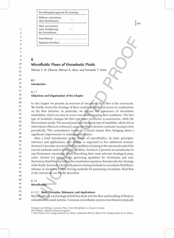
One key benefit of miniaturization is the dramatic reduction in the required fluidsample volume: a linear reduction in the characteristic dimension of the device (L) bya factor of 103 (e.g., from 1 cm to 10 mm) amounts to a volume reduction by a factor of109 (L3). In microfluidic devices, the sample volumes required to fill up a channeltypically range from themicroliter scale down to the nanoliter scale. Furthermore, asa consequence of miniaturization, high surface-to-volume ratios are observed inmicrofluidic devices, as illustrated in Figure 6.1.

The high surface-to-volume ratios typical of microfluidics imply that the balancebetween surface forces (e.g., due to viscous friction and surface tension) and volumeforces (e.g., inertia, gravity) is shifted toward the former. This represents a majordifference relative to macroscale flows, and is crucial for several practical applica-tions. For example, it is possible to fill up a microchannel by capillarity, which wouldbe unthinkable in a macro device – this principle is commonly used in commercialsystems, such as glucose and cholesterolmeters to lead the blood droplet through thecapillary in the test strip where a chemical reaction takes place.

Both macro- and microfluidic flows are commonly driven by pressure gradientsand these are frequently induced using pumps. In microfluidics, special positivedisplacement pumps, such as syringe pumps, are typically employed to pump thefluid through the device. Alternatively, electro-osmosis (EO) can be used to drive andcontrol liquidflows, provided thefluid contains electrolytes. Electrokineticflowshavebeen used for a long time in colloidal and porous systems [3, 4], but have only reallycome of age in microfluidics. The formation of an electric double layer (EDL) allowselectrically conductive fluids to be moved in the microchannels by EO (e.g., [5, 6]).The microchannel walls (as most solid surfaces) acquire an electric charge when incontact with an electrolyte (e.g., water) – an EDL of counter-ions will form sponta-neously at the walls by attracting nearby counter-ions and repelling co-ions. Whenan electric potential is applied across the channel, the ions in the EDL move in thedirection of the electrode of opposite polarity. This causes a motion of the fluid nearthe walls, which in turn creates an advectivemotion of the bulk fluid through viscousforces. The fluid motion exhibits a plug-like profile instead of the characteristicparabolic velocity profile of pressure-drivenflows (PDF). Oncemore, Electro-osmoticflows (EOF) are effective at the microscale because of the dominance of surfaceeffects relative to volume effects. In addition to EO, there are other electrokinetic

Figure 6.1 Surface-to-volume ratio: from macro- to microscale.

132j 6 Microfluidic Flows of Viscoelastic Fluids

1

2

3

4

5

6

7

8

9

10

11

12

13

14

15

16

17

18

19

20

21

22

23

24

25

26

27

28

29

30

31

32

33

34

35

36

37

38

39

40

41

42

43

44

45

effects important at themicroscale, namely electrophoresis, sedimentation potential,and streaming potential. These concepts are thoroughly reviewed by Bruus [6] andthere are many other interesting references and reviews available for electrokineticeffects in microfluidic devices (e.g., [7–11]).

The relative balance between inertial and viscous forces is normally quantified interms of the dimensionless Reynolds number, defined as

Re ¼ rULg

ð6:1Þ

where L is a characteristic dimension of the channel, U is a characteristic velocity,usually the average velocity, and r and g are the density and shear viscosity of thefluid, respectively. The magnitude of the Reynolds number is useful to identify theflow regime – laminar or turbulent. The reduced length scales and the dominance ofviscous forces over inertial forces means that the flows in microfluidic channels aretypically characterized by low to moderate Reynolds numbers (usually smaller than100, and often smaller than 1). At these low Reynolds numbers, the flow is laminarand no turbulence occurs in contrast to what is usually found at the macroscale.Indeed, for laminarflow to be achieved at themacroscale, highly viscousfluids or verylow velocities must be employed, whereas at the microscale, laminar flows can bereadily achieved even with low viscosity fluids such as water. This is a major changerelative to classical transport processes at themacroscale, andmay be an advantage ora disadvantage, depending on the particular application in mind. A number of newtechnological applications have emerged to take advantage of the laminar behavior oftheflow, such as bioassays [12, 13], sorting and separating products of a reaction [1], ormicrofabrication using UV laminar flow patterning [14]. Conversely, many applica-tions require intense mixing, which can be easily (and rapidly) achieved at themacroscale as fluids mix advectively under high inertia flow conditions, but not so atthe microscale where mixing relies mainly on diffusion. Nevertheless, even atReynolds numbers below 100 it is possible to enhance mixing on the basis ofmomentum phenomena such as flow separation as well as viscoelastic flow instabil-ities [15]. The latter will be further discussed in this chapter.

Microfluidic systems have a number of other characteristics that can act asadvantages or challenges depending on the application. For instance, a small con-sumption of reagents can be translated into significant savings both in terms of costand time. This is critical for many applications, namely in biotechnology, whenthe samples to be used are costly or available only in limited amounts (e.g., blood),or when a large number of samples are needed, for example, in high-throughputscreening [16]. Conversely, in applications that involve the detection of biomolecules,as the volumes are reduced, the detection signals become weaker and consequentlynewdetectionmethods (and improved labels when appropriate) need to be developedfor use at the microscale [17]. Furthermore, as the volume-to-surface ratio decreases,liquid evaporation can become an issue if the processes are slow and occur at hightemperatures. Other advantages that arise as a consequence of the reduced lengthscales include significant waste reduction; reduced cost of fabrication; and possibilityof producing highly integrated, disposable, and portable devices. The portability

6.1 Introduction j133

1

2

3

4

5

6

7

8

9

10

11

12

13

14

15

16

17

18

19

20

21

22

23

24

25

26

27

28

29

30

31

32

33

34

35

36

37

38

39

40

41

42

43

44

45

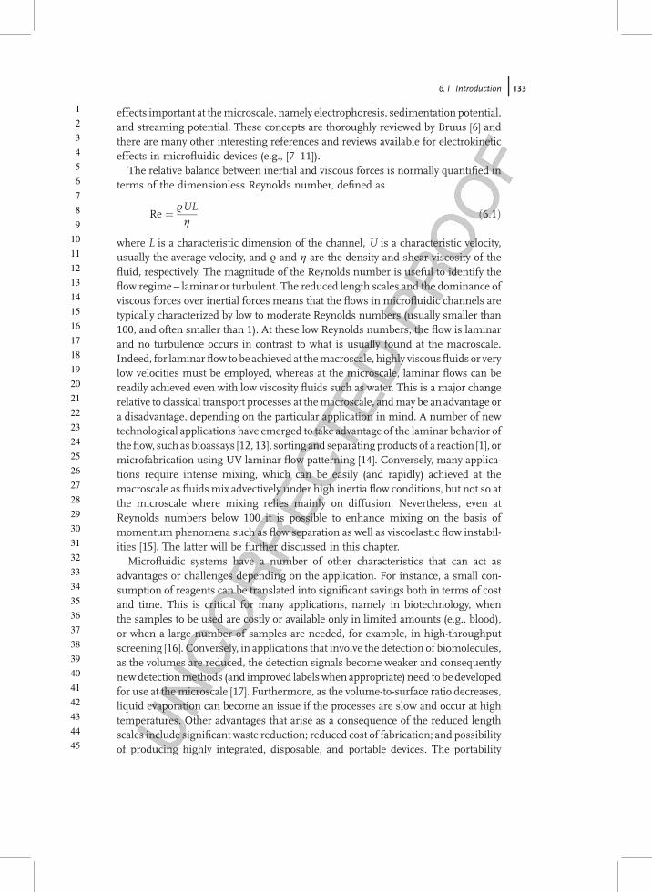
of microfluidic devices results from a combination of the small sizes involvedand the low energy consumptions, which makes this technology suitable for wire-less solutions [18]. On the other hand, one of the main problems in microfluidicsis that the design and fabrication of components are technologically challengingand in most cases cannot simply rely on a scaled down version of their macroscalecounterparts [15]. The effort spent in developing efficient microcomponents is wellapparent in the number of publications dedicated to development of micropumps,micromixers, and so on (cf. reviews [10, 19, 20] and references therein). Likecomponent design, other difficulties in dealing with microfluidic systems are oftena consequence of its youth and can potentially be overcome by further researchand development. Figure 6.2 summarizes the main characteristics of microfluidicsystems as well as the resulting opportunities and challenges associated with fluidicminiaturization.

The advantages identified, together with recent developments in microfabricationtechniques that allow for inexpensive and rapid manufacture of high-quality geom-etries with well-definedmicron-sized features [21–23], have stimulated a remarkable

Microfluidics

• Laminar flow conditions • High surface-to-volume ratio • Strong surface effects • Important electrokinetic effects • Diffusion based processes are

important

Advantages

• Defined and controllable flow • Low sample/reagent consumption • Waste reduction • Effective heat management • High yields and selectivities • High strain rates • Inexpensive and rapid device

fabrication • Low power consumption • High throughput possibility through

parallelization

Disadvantages

• Low detection signals • Liquid evaporation • Difficult to avoid impurities • Difficult component manufacture

and design • Difficult manipulation

Highly integrated and portable devices

Lab on a chip

Figure 6.2 Fluidic miniaturization: opportunities and challenges.

134j 6 Microfluidic Flows of Viscoelastic Fluids

1

2

3

4

5

6

7

8

9

10

11

12

13

14

15

16

17

18

19

20

21

22

23

24

25

26

27

28

29

30

31

32

33

34

35

36

37

38

39

40

41

42

43

44

45

growth and found an extensive range of applications in science and technology, as inbiology,medicine, and engineering [24]. The printing heads of inkjet printers are oneof the most mature commercial applications using microfluidic based systems [25].Other examples include miniaturized systems for production of suspensions andemulsions [26, 27], immunoassays [13, 28], detectionof drugs,flowcytometry [29, 30],dynamic cell separation [31, 32], cell/protein patterning [33], single cell analysis [34],manipulation and analysis of DNAmolecules [35–38], and fuel cells [39]. Many otherapplications have been envisioned and the reader is referred to the literature forfurther details (e.g., [1, 9, 40, 41]).

The commercial impact of microfluidics is becoming increasingly significant andmicrofluidic research aspires to have an impact in the automation of biology andchemistry comparable to the microchip in electronics [1, 42]. Considering onlyapplications in the areas of life sciences and in-vitro diagnostics, the market valuereached 500 million Euros in 2008, and is projected to exceed 2000 million Euros in2014 [43]. More importantly, it is anticipated that the unique characteristics ofmicrofluidic systems have the potential to trigger a range of novel applications inmany areas of science and technology [24]. One of the greatest envisagedmicrofluidictechnological applications consists of a miniaturized laboratory where multipleprocesses can be integrated into a portable platform known as a lab-on-a-chip.Ultimately, this would correspond to shrinking a full production plant or an analysislaboratory into a small chip [44].

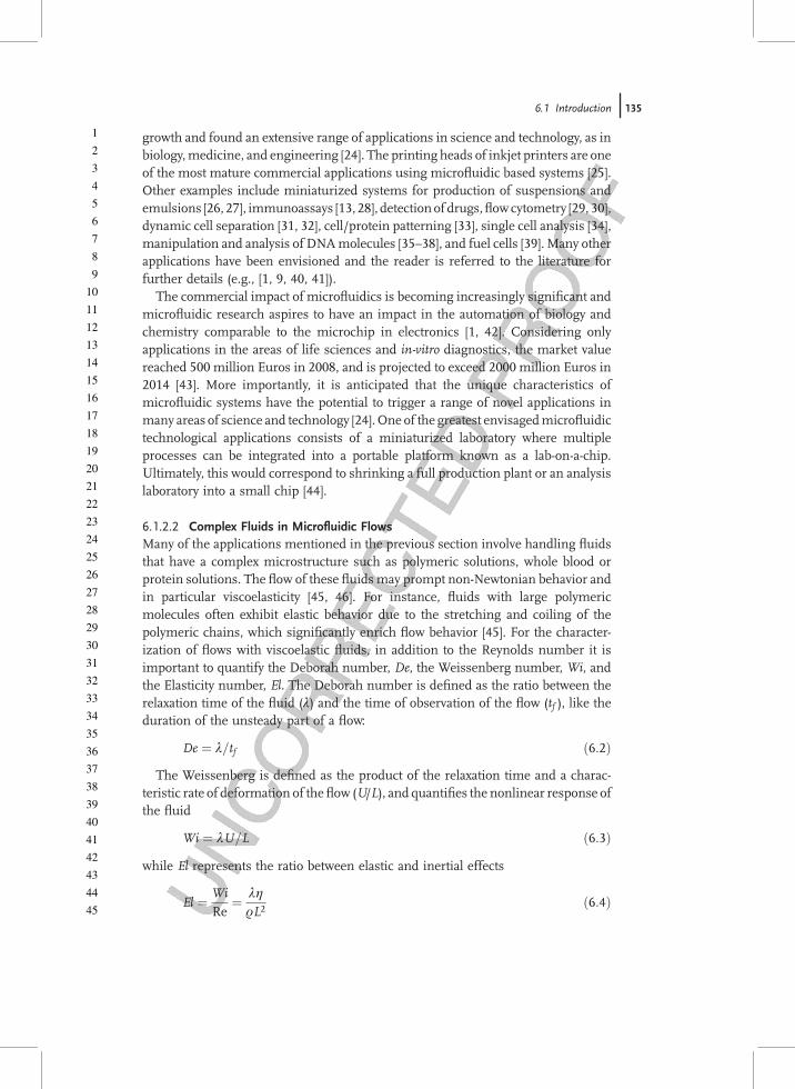
6.1.2.2 Complex Fluids in Microfluidic FlowsMany of the applications mentioned in the previous section involve handling fluidsthat have a complex microstructure such as polymeric solutions, whole blood orprotein solutions. The flow of these fluidsmay prompt non-Newtonian behavior andin particular viscoelasticity [45, 46]. For instance, fluids with large polymericmolecules often exhibit elastic behavior due to the stretching and coiling of thepolymeric chains, which significantly enrich flow behavior [45]. For the character-ization of flows with viscoelastic fluids, in addition to the Reynolds number it isimportant to quantify the Deborah number, De, the Weissenberg number, Wi, andthe Elasticity number, El. The Deborah number is defined as the ratio between therelaxation time of the fluid (l) and the time of observation of the flow (tf ), like theduration of the unsteady part of a flow:

De ¼ l=tf ð6:2ÞThe Weissenberg is defined as the product of the relaxation time and a charac-

teristic rate of deformation of theflow (U/L), and quantifies the nonlinear response ofthe fluid

Wi ¼ lU=L ð6:3Þwhile El represents the ratio between elastic and inertial effects

El ¼ WiRe

¼ lg

rL2ð6:4Þ

6.1 Introduction j135

1

2

3

4

5

6

7

8

9

10

11

12

13

14

15

16

17

18

19

20

21

22

23

24

25

26

27

28

29

30

31

32

33

34

35

36

37

38

39

40

41

42

43

44

45

In steady Eulerian flows with unsteady Lagrangian characteristics, such as theflow in a contraction, the Weissenberg and Deborah numbers are proportional and,as pointed out by Dealy [47], there has been widespread misapplication of bothdimensionless numbers. The small length scales together with the high deforma-tion rates and short transit times characteristic of microfluidic systems enable thegeneration of high Deborah or Weissenberg number flows while keeping theReynolds number low, leading to high El flows. These distinctive flow conditionsresult in the ability to promote strong viscoelastic effects, which are not masked byfluid inertia, even in low viscosity/elasticity fluids that would in contrast exhibitNewtonian-like behavior at the equivalent macroscale [48–52]. The dimensionlessWi–Re parameter space is depicted in Figure 6.3, where the operation regions formacro- and microscale flows are distinguished. It is clear that the geometric scale ofmicrofluidic devices results in flows that are distinct from those seen at themacroscale, particularly when they are extension dominated [48, 49, 52–55].

6.1.2.3 Continuum ApproximationWe end this introduction by analyzing the validity of the continuum approximationformodelingfluidflowat themicroscale. The continuumapproximation implies thatfluid and flow properties (such as density, viscosity, velocity, stresses, etc.) are definedeverywhere in space and vary continuously throughout space [56]. Flows can bemodeled by the continuum approximation, also using molecular dynamics, whichconsiders a collection of individual interacting molecules, or more recently as acombination of both approaches using multiscale techniques [57, 58]. Adopting thecontinuum approach is generallymuch simpler, it easily considers large systems and

Wi

Macro

Micro

Boger fluid

Newtonian fluid

Bog

er f

luid

Re

Figure 6.3 Operational regions in the Wi–Reparameter space. The dotted line correspondsto Newtonian fluids (Wi¼ 0) and the dashedlines represent a Boger fluid (i.e., viscoelastic

fluidwith constant viscosity, cf. Section 6.3)withlow viscosity and low relaxation time in flows atthe micro- and macroscale.

136j 6 Microfluidic Flows of Viscoelastic Fluids

1

2

3

4

5

6

7

8

9

10

11

12

13

14

15

16

17

18

19

20

21

22

23

24

25

26

27

28

29

30

31

32

33

34

35

36

37

38

39

40

41

42

43

44

45

is less time consuming than the other techniques, which are still not feasible formany realistic applications and for a sufficiently large number of molecules [42].However, in simplified terms, for the continuum approximation to hold two mainconditions need to bemet: (i) themolecules need to be small enough compared to thecharacteristic length scale of the flow; (ii) the number of molecules inside each fluidelement needs to be large enough. In classical fluid mechanics at the macroscale,these conditions are generally satisfied and the continuum approach generallyholds [56].

The same is also true in many microfluidics systems, especially those operatingwith liquids. For example, in Newtonian liquid flows at micrometer-length scales ithas been well established that under standard conditions the basic continuum lawsgoverning fluid flow, expressed by the equations of mass conservation and momen-tum, and the no-slip boundary condition at walls, remain valid [25, 51, 58–60]. Forwater, the continuum assumption is not expected to break down when the channeldimensions are above 1 mm [5]. For molecules such as water, the ratio of molecularsize (�0.3 nm) to geometric length scale (typically on the order of tens to hundreds ofmicrons) is �10�5–10�6. As such, it is considered that there are enough moleculesat each location within the flow (the concept of fluid particle as a small volume witha large number of molecules is useful) and that the molecules are small enoughto treat the flow under the continuum theory [24]. This remains valid even formore complex fluid flows, including high-molecular-weight polymeric solutions, asattested by the agreement between experimental andnumerical data inmicrofluidics,which provides further credibility to this assumption [55, 61, 62].

However, there are a number of exceptions to the validity of the continuumhypothesis as the characteristic length scales of theflowdecrease significantly [63, 64],namely when considering gas flows or gas–liquid flows, in which the gas density isvery low compared to liquids. In gas flows, the Knudsen number representing theratio between the mean free path of molecules and the characteristic length scale ofthe flow is used to evaluate the validity of the continuum approach. Based on theexperimental evidence, it is generally accepted that for Knudsen numbers below 0.01the continuum approximation is valid. For Knudsen numbers above 0.01, there aredeviations to the continuum theory, which are handled initially with corrections andsubsequently by other theories that describe microscale flow [57, 58, 65].

The other notable exception is related to complex fluids that are composed of largeparticles in suspension (e.g., red blood cells) or long molecules such as DNA or evenpolymers of high molecular weight. The radius of gyration of a polymer chain or thecharacteristic radius of a suspended particle typically varies from 1nm to 10mm. Assuch, for particle/molecule sizes in the high end of the range, assuming a continuumcan be misleading since the working fluid may not be well approximated asmicrostructurally homogeneous [66]. In this case, other methods should be usedto properly model the flow.

Although it is important to be aware of cases where the validity of the continuumapproximation breaks down, in all situations of relevance to this chapter, the typicaldimensions of molecules and channels are within the range of application of thecontinuum approach.

6.1 Introduction j137

1

2

3

4

5

6

7

8

9

10

11

12

13

14

15

16

17

18

19

20

21

22

23

24

25

26

27

28

29

30

31

32

33

34

35

36

37

38

39

40

41

42

43

44

45

6.2Mixing in Microfluidics

6.2.1Challenges of Micromixing

Efficient mixing may be defined as a procedure for homogenizing an otherwiseinhomogeneous system in the shortest possible amount of time and using theleast amount of energy [67]. Mixing is required for many practical applications, inparticular in association with chemical reaction. Furthermore, rapid mixing is oftenan essential requirement to achieve a good performance in many microfluidicapplications, namely for biochemistry analysis, drug delivery, sequencing andsynthesis of nucleic acids, protein folding, and chemical analysis or synthesis.

In macroscale devices, fluid mixing can often be readily achieved by inducingturbulent flow. In contrast, though not impossible, turbulence is more difficult toreach in microfluidic systems due to the reduced length scale of the channels.Additionally, in many microfluidic applications associated with biological systems,the velocity of theflow cannot be too high since high velocitiesmay lead to large shearstresses that can damage cells and compromise their function [15]. Therefore, in thelargemajority of cases,microfluidic flows take place in the laminar regime, and oftenat low Reynolds numbers.

The steady laminar flow of Newtonian fluids in ducts is deterministic. When theReynolds numbers are low, fluids do not mix advectively when different streamscome together in a straight microchannel. Instead, the fluid streams flow in parallelas shown in Figure 6.4, with mixing occurring only due to molecular diffusionacross the interface between the streams. At this point, it is useful to introduce thedimensionless P�eclet number, which expresses the relative importance of theconvective over the diffusive mass transport

Pe ¼ UL=D ð6:5Þwhere D is the diffusion coefficient. For typical microfluidic flow conditions, Pe isgenerally higher than 10, which means that the diffusion process acts more slowly

Figure 6.4 Junction of two Newtonian fluid streams in a microfluidic device under low Re flowconditions.

138j 6 Microfluidic Flows of Viscoelastic Fluids

1

2

3

4

5

6

7

8

9

10

11

12

13

14

15

16

17

18

19

20

21

22

23

24

25

26

27

28

29

30

31

32

33

34

35

36

37

38

39

40

41

42

43

44

45

than the hydrodynamic transport. Additionally, advection is often parallel to themainflow direction and is not useful for the transversal mixing process [19].

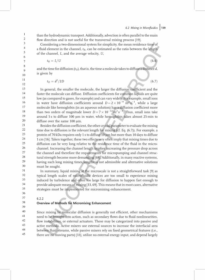
Considering a two-dimensional system for simplicity, the mean residence time ofa fluid element in the channel, tR, can be estimated as the ratio between the lengthof the channel, L, and the average velocity, U,

tR ¼ L=U ð6:6Þ

and the time for diffusion (tD), that is, the time amolecule takes to diffuse a distance d,is given by

tD ¼ d2=2D ð6:7Þ

In general, the smaller the molecule, the larger the diffusion coefficient and thefaster the molecule can diffuse. Diffusion coefficients for common liquids are quitelow (as compared to gases, for example) and can vary widely. For example, small ionsin water have diffusion coefficients around D¼ 2� 10�9 m2 s�1, while a largemolecule like hemoglobin (in an aqueous solution) has a diffusion coefficient morethan two orders of magnitude lower D¼ 7� 10�12m2 s�1. Thus, small ions takearound 5 s to diffuse 100 mm in water, while hemoglobin takes almost 25min todiffuse over the same 100 mm.

Besides the diffusion coefficient, the other crucial parameter to evaluate themixingtime due to diffusion is the relevant length for mixing (cf. Eq. (6.7)). For example, aprotein of 70 kDa requires only 1 s to diffuse 10 mm but more than 10 days to diffuse1 cm [16]. Taken together, these two effects very often imply that mixing times due todiffusion can be very long relative to the residence time of the fluid in the micro-channel. Increasing the channel length implies increasing the pressure drop acrossthe channel and therefore the requirements for micropumping and channel struc-tural strength becomemore demanding [68]. Additionally, inmany reactive systems,having such long mixing times/lengths is not admissible and alternative solutionsmust be sought.

In summary, liquid mixing at the microscale is not a straightforward task [9] astypical length scales of microfluidic devices are too small to experience mixinginduced by turbulence and often too large for diffusion to happen fast enough toprovide adequatemeans ofmixing [33, 69]. Thismeans that inmost cases, alternativestrategies must be implemented for micromixing enhancement.

6.2.2Overview of Methods for Micromixing Enhancement

Since mixing by molecular diffusion is generally not efficient, other mechanismsneed to be brought into action, such as secondary flows due to fluid nonlinearities,flow instabilities, or external actuators. These may be categorized into passive andactive methods. Active mixers use external sources to increase the interfacial areabetween fluid streams, while passive mixers rely on fixed geometrical features (i.e.,there are no moving parts) [33], utilize no external energy input, and depend largely

6.2 Mixing in Microfluidics j139

1

2

3

4

5

6

7

8

9

10

11

12

13

14

15

16

17

18

19

20

21

22

23

24

25

26

27

28

29

30

31

32

33

34

35

36

37

38

39

40

41

42

43

44

45

on the mechanism used for generating fluid flow through the microchannel [24].A good introduction to the general theme of mixing is presented by Ottino [70],and by Nguyen [15] for the particular case of micromixing, and is only brieflysummarized below.

One possible approach to enhance mixing, inspired by macromixers, is to useactive methods to perturb the low Reynolds number flows. Active mixing requiresexternal forcing to induce a flow disturbance and hence increases the amount oftransverse flowwithin the channel. These forcesmay come frommovingmechanicalparts and/or external actuators [71]. Active mixers usually produce high levels ofmixing, but the systems are considerably more complex, may be difficult to integrateinto microfluidic devices, and can be expensive to manufacture [24]. A particularchallenge is related to the dominance of surface effects over volume effects as thesystems are miniaturized. As a consequence, actuation concepts based on volumeforces (e.g., magnetic stirrer), which are widely used at the macroscale, become lessefficient at the microscale [15].

The actuator for active mixing can be a pump or works as an energy source,for example, pulsating side flow [72], micropumping for stopping and restartingthe flow [73], application of unsteady electric fields acting on the fluid or onsuspended particles [74], application of potential differences across pairs of electro-des within the microchannel in the presence of an external magnetic field [75, 76],application of thermal gradients to induce disturbances in the flow using eitherthermopneumatic actuators (based on the thermal expansion of gases), thermal-expansion actuators (based on the thermal expansion of solids) and bimetallicactuators (based on the difference in thermal coefficient of expansion of two bondedsolids) [15], or application of acoustic fields [77, 78]. For further details, the reader isreferred to [15, 79]. Active principles can also obviously be used in combination withpassive techniques.

Another alternative to reduce mixing times is to induce stirring by chaoticadvection [80], with final mixing by diffusion, a process that has also been used inmicrofluidics [81, 82] and requires a non-negligible Reynolds number since chaoticadvection is inherently a nonlinear inertial effect. This is usually accomplished invarious ways, depending on the flow Reynolds number, but invariably the flowbecomes time-dependent and can also be three-dimensional [19]. If the Reynoldsnumber is low and the fluid is Newtonian, the use of 2D obstacles is usually insuf-ficient to create chaotic advection and enhancemixing. Asymmetric and 3D arrange-ments of flow perturbations, such as grooves, obstacles, and duct twists becomenecessary to impart the stretching, reorientation, and randomizationmechanisms ofdistributivemixing [19, 83]. Micromixing in Newtonian fluids by chaotic advection isreviewed in detail by Nguyen [15].

Fluids in microsystems very often contain additives that impart non-Newtoniancharacteristics to the fluids and, in particular, viscoelasticity. These rheologicalcharacteristics introduce nonlinearities that can be explored to dramatically changethe flow dynamics, and in particular to enhance mixing [1, 54, 84]. The elasticity ofthe fluids is characterized, among other things, by the appearance of anisotropicnormal stresses, which produce secondary flows [85] and/or elastic instabilities even

140j 6 Microfluidic Flows of Viscoelastic Fluids

1

2

3

4

5

6

7

8

9

10

11

12

13

14

15

16

17

18

19

20

21

22

23

24

25

26

27

28

29

30

31

32

33

34

35

36

37

38

39

40

41

42

43

44

45

at extremely low Reynolds number. Although weak, these secondary flows helpthe appearance of flow instabilities and reduce mixing times, because they createconditions similar to those of chaotic advection, that is, 3D flow which we call herechaotic elastic flow (inertia is negligible). The elastic instabilities have been shownto exist even in the absence of inertia and are associated with strong curvatureof streamlines and large normal stresses [86]. When the elastic instabilities becomevery intense, reaching a saturated nonlinear state, fluctuations even become randomover a wide range of length and time scales [87], very much like inertial turbulence,in spite of negligible Reynolds numbers. This has prompted Groisman andSteinberg [88] to call it �elastic turbulence.� So, elastic effects are used to reducethe critical conditions for the existence of chaoticflowand enhancedmixing, allowingthe use, at lower Reynolds numbers, of passive techniques usually associated withhigher Reynolds number flows. This type of passive mixing is discussed in detail inSection 6.5. Before that, however, we introduce in Section 6.3 some basic conceptsabout non-Newtonian fluids, as well as the governing equations required for flows ofcomplex fluids (Section 6.4).

6.3Non-Newtonian Viscoelastic Fluids

In this section, we present a brief overview of the rheology of non-Newtonian fluids.More detailed descriptions are found in [45, 46], among others. Rheometry is alsodescribed in [89, 90].

The rheology of fluids is assessed through their behavior in a small set ofcontrollable (and quasi-controllable) flows, whose kinematics are known andindependent of fluid properties. For shear-based properties, this is the Couetteflow schematically shown in Figure 6.5 in the planar (2D) version. Technologically,the Couette flow is usually implemented in an axisymmetric version, as in theconcentric cylinders, cone–plate, or plate–plate geometries for which the appliedtorque and rotational speed are directly proportional to the shear stress andshear rate, respectively. The use of small gaps in these geometries ensures acontrollable flow and a nearly constant shear rate across the gap. For extensional-based properties the ideal flow is a purely extensional flow, such as the uniaxialextension, but it is not always possible to implement it easily, especially for low-viscosity fluids.

U1x2u1 = U1H

x2

x1

H

Figure 6.5 Plane Couette flow and coordinate system.

6.3 Non-Newtonian Viscoelastic Fluids j141

1

2

3

4

5

6

7

8

9

10

11

12

13

14

15

16

17

18

19

20

21

22

23

24

25

26

27

28

29

30

31

32

33

34

35

36

37

38

39

40

41

42

43

44

45

6.3.1Shear Viscosity

Shear viscosity is defined as the ratio between shear stress (t12) and the shear rate ( _c)in the Couette flow of Figure 6.5, where subscripts 1 and 2 denote streamwise andtransverse directions, respectively:

g ¼ t12du1=dx2

¼ t12U1=H

¼ t12_c

ð6:8Þ

Typically, non-Newtonian fluids have a shear-thinning behavior with a low shearrate constant viscosity plateau, as shown in Figure 6.6. A second lower constantviscosity plateau at high shear rates is also frequent, but often this is not observed inrheometricflows before the onset offlow instabilities. Some suspensions of irregularsolids, or surfactant solutions, exhibit a shear-thickening behavior, but this is oftenlimited to a narrow range of shear rates.

There are materials for which the first Newtonian plateau of the shear viscosity isnot observed, and the shear viscosity grows to infinity at vanishingly small shear rates.Thesematerials possess some formof internal structure forwhich aminimumstressis required prior to yielding – the yield stress – and often their viscosity depends notonly on the shear rate but also on time – thixotropy or anti-thixotropy, depending onwhether the shear viscosity increases or decreases over time. Examples are tooth-paste, mayonnaise, blood, and suspensions of particles, in which the effect isenhanced if macromolecules are present. Dilute and semidilute polymer solutionsdo not exhibit yield stress and thixotropy, so these properties will not be considered

10-3

10-2

10-1

100

10-1 100 101 102 103 104

0.2% XG0.4% CMC

η (P

a.s)

γ (s-1)

Newtonian

Second Newtonianplateau

Law of Carreau

Shear-thickeningbehavior

.

Figure 6.6 Shear viscosity of aqueous solutions of 0.2% by weight xanthan gum (XG) and 0.4% byweight carboxy methyl cellulose (CMC) and typical behavior of some rheological models.

142j 6 Microfluidic Flows of Viscoelastic Fluids

1

2

3

4

5

6

7

8

9

10

11

12

13

14

15

16

17

18

19

20

21

22

23

24

25

26

27

28

29

30

31

32

33

34

35

36

37

38

39

40

41

42

43

44

45

further. The interested reader is referred to Larson [46] and additional papers onissues and techniques involving yield stress fluids [91–95].

6.3.2Normal Stresses

Viscoelastic fluids develop normal stresses in shear flow, which are known within aconstant value, so their differences are the useful material properties. For a pureshearflowas illustrated in Figure 6.5, thefirst normal stress difference (N1) is definedas the difference between the streamwise normal stress (t11) and the transversenormal stress (t22), and gives rise to the material property designated as first normalstress difference coefficient, Y1:

Y1 � N1

_c2¼ t11�t22

_c2ð6:9Þ

The second normal stress difference is N2 � t22�t33 and the correspondingcoefficient isY2 ¼ N2= _c

2. N2 is usually small, with maximum values not exceeding20% ofN1 and with an opposite sign toN1. Measurement ofN2 is difficult and can bedone using a special cone–plate apparatus [96].

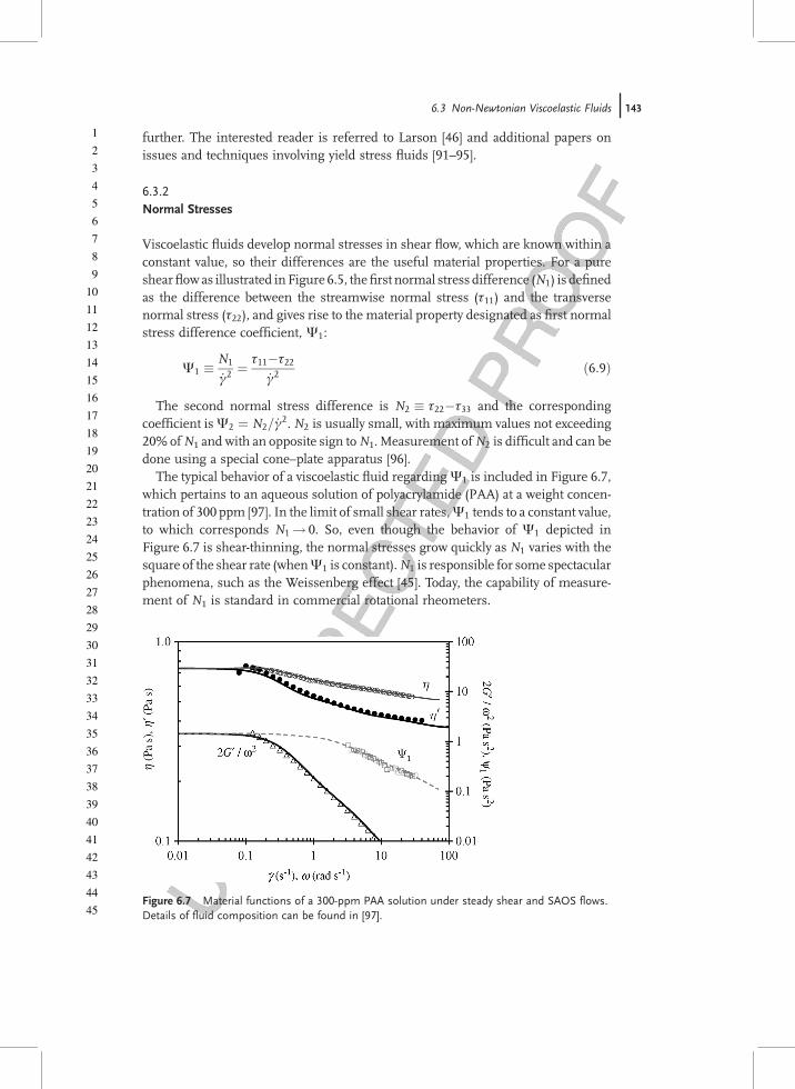
The typical behavior of a viscoelastic fluid regardingY1 is included in Figure 6.7,which pertains to an aqueous solution of polyacrylamide (PAA) at a weight concen-tration of 300 ppm [97]. In the limit of small shear rates,Y1 tends to a constant value,to which corresponds N1 ! 0. So, even though the behavior of Y1 depicted inFigure 6.7 is shear-thinning, the normal stresses grow quickly as N1 varies with thesquare of the shear rate (whenY1 is constant).N1 is responsible for some spectacularphenomena, such as the Weissenberg effect [45]. Today, the capability of measure-ment of N1 is standard in commercial rotational rheometers.

Figure 6.7 Material functions of a 300-ppm PAA solution under steady shear and SAOS flows.Details of fluid composition can be found in [97].

6.3 Non-Newtonian Viscoelastic Fluids j143

1

2

3

4

5

6

7

8

9

10

11

12

13

14

15

16

17

18

19

20

21

22

23

24

25

26

27

28

29

30

31

32

33

34

35

36

37

38

39

40

41

42

43

44

45

6.3.3Storage and Loss Moduli

In small amplitude oscillatory shear (SAOS) flow of a viscoelastic fluid, an oscillat-ing shear stress, t ¼ t0 sinðv tÞ, is applied to one of the walls of the Couette cell(alternatively, an oscillatory deformation can be applied, c ¼ c0 sinðv tÞ, and thecorresponding shear stress measured). The ensuing fluid deformation will be givenby c tð Þ ¼ c0 sin v tþ dð Þ, and is out of phase by d relative to the applied stress.Provided the amplitude of deformation is small, the response of thematerial dependsonly on the forcing frequency and the resulting storage (G0) and loss (G00) moduli aremathematically defined as

G0 ¼ v g00 � t0c0

cos d; G00 ¼ v g0 � t0c0

sin d ð6:10Þ

which measure the amount of energy stored reversibly by the material (G0, defor-mation in phase with the stress) and consequently can be recovered, and the energyirreversibly lost by viscous dissipation (G00, deformation out of phase with the stress).Sometimes the components g0 and g00 of the complex dynamic viscosity (g�) are usedinstead, where g� ¼ g0�i g00, with i representing the imaginary number (i2 ¼ �1).

For a Newtonian fluid, the response in this test would be obvious (G0 ¼ 0,G00 ¼ t0=c0) so the loss angle (d) would be maximum and given by d ¼ p=2 (notethat tan d ¼ G00=G0).

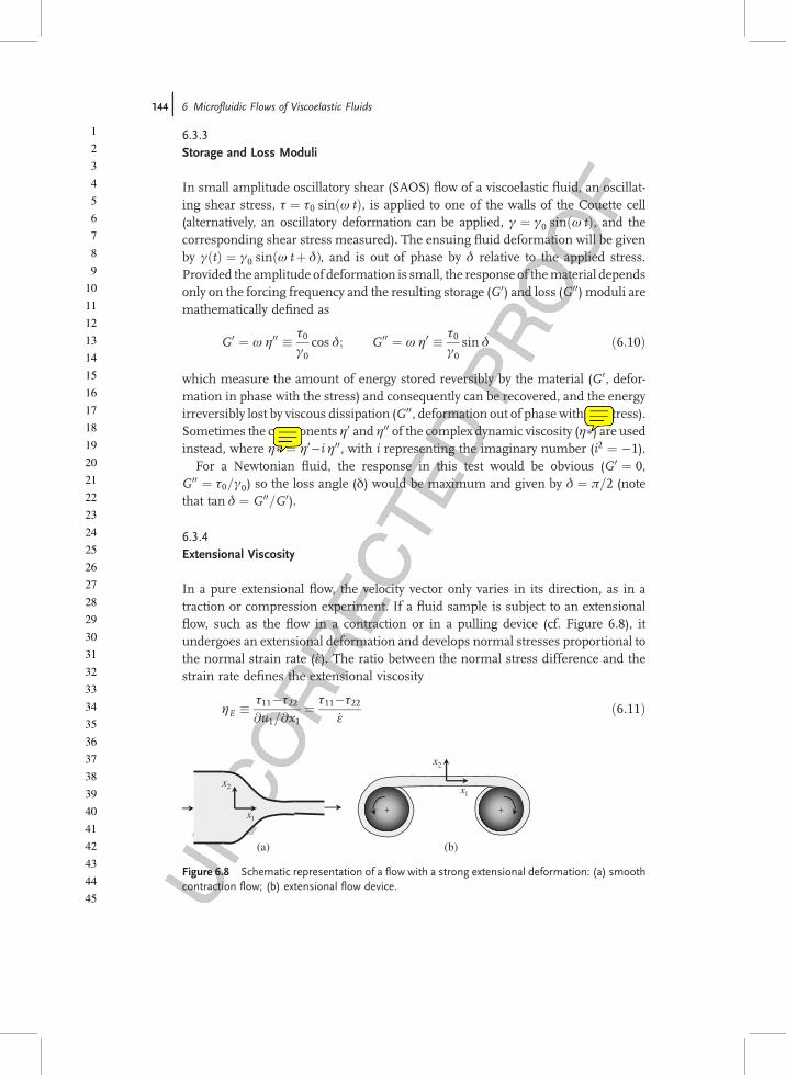
6.3.4Extensional Viscosity

In a pure extensional flow, the velocity vector only varies in its direction, as in atraction or compression experiment. If a fluid sample is subject to an extensionalflow, such as the flow in a contraction or in a pulling device (cf. Figure 6.8), itundergoes an extensional deformation and develops normal stresses proportional tothe normal strain rate ( _e). The ratio between the normal stress difference and thestrain rate defines the extensional viscosity

gE � t11�t22@u1=@x1

¼ t11�t22_e

ð6:11Þ

1x

2x

(a)

2x

1x

(b)

Figure 6.8 Schematic representation of a flow with a strong extensional deformation: (a) smoothcontraction flow; (b) extensional flow device.

144j 6 Microfluidic Flows of Viscoelastic Fluids

1

2

3

4

5

6

7

8

9

10

11

12

13

14

15

16

17

18

19

20

21

22

23

24

25

26

27

28

29

30

31

32

33

34

35

36

37

38

39

40

41

42

43

44

45

Note that all fluids, including Newtonian fluids, have a nonzero extensionalviscosity. For Newtonian fluids, the uniaxial extensional viscosity equals three timesthe shear-viscosity, so no distinction is required, but for viscoelastic fluids the ratiobetween the extensional and shear viscosities, called the Trouton ratio, varies with therate of deformation and can largely exceed the value of three, attaining sometimesvalues of the order of 100 or higher. An impressive consequence of a very highextensional viscosity is the tubeless siphon experiment [45].

The measurement of the extensional viscosity is not easy, because it is difficultto ensure that fluid particles are under a constant strain rate for a sufficientlylong time to eliminate transient start-up effects, especially at high strain rates.Additionally, for the mobile systems of interest here it is difficult to impose a con-stant strain rate flow and so the extensional viscosity can only be directly measuredwith such devices as the capillary break up extensional rheometer (CaBER) [98]. Avariant of the CaBER is the filament stretching extensional rheometer (FiSER)based on the work of Tirtaatmadja and Sridhar [99], where the fluid filamentbetween plates is deformed as the plates move with a velocity increasing expo-nentially with time. This allows the measurement of strain-dependent extensionalviscosity [100].

Alternatively, there are flows with a strong extensional nature from which anextensional viscosity indexer can be obtained, such as the pressure drop enhance-ment in a contraction flow or the tensile force required to sustain fluid stretching inthe space between two nozzles in the opposed jet rheometer, but in these flows thefluids are not subject to a constant strain rate and the flow is contaminated bysecondary effects that may overwhelm the main measurement. In contrast, the highconsistency of polymer melts facilitates the integrity of fluid samples under uniaxialextension and a number of devices can be used tomeasure their extensional viscosity,such as the Sentmanat device [101].

6.3.5Other Rheological Properties

The rheological properties discussed can today be reliably measured and arestandard. However, it is clear to rheologists and fluid dynamicists alike that the setdoes not guarantee that if a rheological constitutive equation is able to predict all ofthem for a particularfluid, it will be able to predict accurately all types offlowwith thatfluid [102, 103], a situation quite similar to the prediction of Newtonian turbulentflows. This indicates the need for other fluid properties, especially those related totime-dependency and nonlinear effects.

Other tests, such as the creep and the stress relaxation flows in shear and strain,are good examples. One may also consider the response of fluids to a sequenceof steps in normal or shear strain, since here the response of fluids is different fromthat to a single step. To assess nonlinear viscoelasticity, meaningful interpretationof data from large amplitude oscillatory shear flow (LAOS) is currently underdevelopment [104].

6.3 Non-Newtonian Viscoelastic Fluids j145

1

2

3

4

5

6

7

8

9

10

11

12

13

14

15

16

17

18

19

20

21

22

23

24

25

26

27

28

29

30

31

32

33

34

35

36

37

38

39

40

41

42

43

44

45

6.4Governing Equations

Viscoelastic fluid flow is governed by the momentum and continuity equationstogether with a rheological constitutive equation adequate for the fluid. If heattransfer is involved, the energy equation must be included with the correspondingthermal constitutive equation, usually Fourier�s heat law. To consider chemicalreaction, the mass conservation equation for each chemical species needs to besolved in combination with the mass transport constitutive equation, usually Fick�slaw. To assess mixing performance, it may be necessary to solve a transport equationfor an adequate scalar. These equations are coupled in a variety of ways: dependenceof fluid properties on temperature, molecular orientation and/or fluid composition,through new terms in the governing equation, such as buoyancy in the momentumequation or extra terms in the constitutive equation, which can be traced back to theeffect of temperature on the mechanisms acting at microscopic level. The treatmentof these extra terms of the constitutive equations is an advanced topic not consideredhere. For a more in-depth discussions, the reader is referred to [105–107].

In general, the fluid dynamics and heat transfer problems are coupled and the setof governing equations has to be solved simultaneously. For a general flow problem,this can only be done numerically, but under simplified conditions, such astemperature-independent fluid properties (a good approximation, if temperaturevariations are small), it is possible to solve for the flow without consideration for thethermal problem (although not the other way around). Other times, the solution canstill be obtained assuming temperature-independent properties, but a correction isintroduced to compensate for the neglected effect. This is a fairly successful approachfor simple geometries and simple fluids (such as inelastic fluids), but for viscoelasticfluids a more exact approach may be required for accurate results [108].

The governing equations are presented in the next sections in tensor notation forgenerality. The reader is referred to the appendices of Bird et al. [45, 109, 110] for anextensive presentation of their form in various coordinate systems.

6.4.1Continuity and Momentum Equations

The continuity equation is written as

@r

@tþr � ruð Þ ¼ 0 ð6:12Þ

and the momentum equation as

@ ruð Þ@t

þrðu �rÞu¼�rpþrgþr�ttþreE�12E �E20r2 þ20

2r r

@ 2@r

E �E� �

ð6:13Þwhereu is the velocity vector, p is the pressure,r is thefluid density, and thefluid totalextra stress (tt) is given by an adequate rheological constitutive equation. The last

146j 6 Microfluidic Flows of Viscoelastic Fluids

1

2

3

4

5

6

7

8

9

10

11

12

13

14

15

16

17

18

19

20

21

22

23

24

25

26

27

28

29

30

31

32

33

34

35

36

37

38

39

40

41

42

43

44

45

three terms on the right-hand side take electrokinetic effects into account, where redenotes the net electric charge distribution within the fluid, E represents the appliedelectric field (or induced streaming potential in flows with electroviscous effects), 20

is the dielectric permittivity of vacuum, and 2 is the dielectric constant of the fluid.The last term accounts for permittivity variations with fluid density and is only rele-vant at gas–liquid interfaces or in ionized gas flows, whereas the penultimate termaccounts for spatial variations in the dielectric constant of the fluid. Thus, for incom-pressible fluids of constant dielectric permittivity only the first of the three terms isrequired, which is known as Lorentz force.

The applied electric field intensity can be related to the imposed electric potentialE ¼ �rw and similarly the induced charge is related to the induced potential .In this chapter, we will assume that they are independent of each other and there-fore they can be linearly combined into the total electric potentialW ¼ wþ . This isadmissible when the EDL is thin, and also requires a weak applied streamwisegradient of electrical potential, that is, Dw=L � 0=�, where Dw is the potentialdifference of the applied electricalfield,L is the distance between the electrodes, and �is the Debye layer thickness. In this case, the transverse charge distribution isessentially determined by the potential at the wall, 0, the so-called zeta potential.If the local EOF velocities are small and/or parallel to the walls, as in thin EDLs,the effect of fluid motion on the charge distribution can also be neglected. Thesesimplifications are part of the so-called standard electrokinetic model, in which caseEq. (6.13) becomes

@ ruð Þ@t

þ rðu � rÞu ¼ �rpþrgþr � tt�rerW ð6:14Þ

6.4.2Rheological Constitutive Equation

The fluid total extra stress (tt) is given as the sum of an incompressible solventcontribution having a viscosity coefficient gs and a polymer/additive stress contri-bution tp, as

tt ¼ 2gs IID; IIIDð ÞDþ tp ð6:15ÞThe solvent viscosity coefficient in Eq. (6.15) has been made to depend on the

second and third invariants (IID, IIID) of the rate of deformation tensorD defined as

D ¼ 12

ruþruT� � ð6:16Þ

to consider both the possibility of having a Newtonian (constant viscosity) or a non-Newtonian (variable viscosity) solvent. In this way, Eq. (6.15) includes the class ofinelastic non-Newtonian fluids known as generalized Newtonian fluids (GNF) forwhich the polymer contribution is set to zero (tp ¼ 0). Then, the viscosity coefficientdepends on invariants of the rate of deformation tensor, themost common being thesecond invariant, defined in the next section. For viscoelastic fluids, gs is set to zero

6.4 Governing Equations j147

1

2

3

4

5

6

7

8

9

10

11

12

13

14

15

16

17

18

19

20

21

22

23

24

25

26

27

28

29

30

31

32

33

34

35

36

37

38

39

40

41

42

43

44

45

for polymer melts or to a nonzero constant when dealing with a polymer solutionbased on a Newtonian solvent.

Usually the non-Newtonian fluids are treated as incompressible fluids, so the con-tinuity equation simplifies tor �u ¼ 0. Some very limited phenomena may requireconsideration of liquid compressibility, an issue not considered here.

6.4.2.1 Generalized Newtonian Fluid ModelThe purely viscous GNF model is defined in Eq. (6.15) with tp ¼ 0 and the fluidviscositygs IID; IIIDð Þdepending on invariants of the rate of deformation tensor [111].Themost commonmodels consider only dependence on the second invariant andwecan write many of them in a compact form as

gs IIDð Þ ¼ g1�g2ð Þ aþ LIIDð Þa½ n�1a þg2 with IID �

ffiffiffiffiffiffiffiffiffiffiffiffiffiffi2D : D

pð6:17Þ

Equation 6.17 includes the Newtonian fluid model (viscosity coefficient g),the Ostwald de Waele power law (consistency index K and power index n), theCarreau–Yasudamodel (zero shear viscosityg0, infinite shear rate viscosityg1, powerindex n, transition coefficient a, and transition time scaleL), the simplified Carreaumodel and the Sisko model, with the corresponding coefficients given in Table 6.1.

6.4.2.2 Viscoelastic Stress ModelsThe previous constitutive models cannot predict viscoelastic characteristics, such asany shear-induced normal stresses in Couette flow, or memory effects. There is aclass of models, which is still explicit on the stress tensor that can predict some ofthese elastic effects.One suchmodel, theCriminale–Eriksen–Filbey (CEF) equation,should only beused in steady shearflow inwhich case it provides accurate results [45].The CEF model can be written as

t ¼ 2g _cð ÞD�Y1 _cð ÞDr þ 4Y2 _cð ÞD2 ð6:18Þwith _c � IID and D

rrepresenting the upper-convected derivative of D, defined as

Dr � @D

@tþ u � rð ÞD�ruT �D�D � ru ð6:19Þ

Table 6.1 Values of parameters in generalized viscosity function of Eq. (6.17) for some typicalviscosity models.

N a a g1 g2 L ��

Newtonian 1 Any Any g 0 AnyPower law N Any 0 � 0 � K ¼ g1L

n�1

Carreau–Yasuda N Any 1 g0 g1 L

Simplified Carreau N 2 1 g0 0 L

Sisko n Any 0 � g1 � K ¼ ðg1�g2ÞLn�1

148j 6 Microfluidic Flows of Viscoelastic Fluids

1

2

3

4

5

6

7

8

9

10

11

12

13

14

15

16

17

18

19

20

21

22

23

24

25

26

27

28

29

30

31

32

33

34

35

36

37

38

39

40

41

42

43

44

45

Other stress explicit models for viscoelastic fluids are contained in Eq. (6.18), suchas the second-order fluid (constant g, Y1, and Y2) or the Reiner–Rivlin equation(Y2 ¼ 0). The use of thesemodels should be restricted toweakly elasticfluids and lowWeissenbergnumberflows, that is, tofluids deviating slightly fromNewtonian and toslow flows, since outside these conditions they lead to physically incorrect predic-tions. So, these models are essentially useful to investigate deviations from thebehavior of Stokes fluids.

More useful are the integro-differential viscoelastic fluid models. The polymericcontribution to the extra-stress tensor in Eq. (6.15) can in general be represented as aset of N modes

tp ¼XNk¼1

tk ð6:20Þ

where each polymer mode obeys a rheological equation of state of integral ordifferential nature. An example of the latter is the following general equation:

f tr tð Þtþ l

F tr t; L2ð Þ t& þ al

gpt2 ¼ 2gpD ð6:21Þ

which includes such models as the upper-convected Maxwell (UCM) model, thePhan-Thien–Tanner model (PTT), the Johnson–Segalman (JS) model, the Giesekusmodel or the FENE-MCR model, according to Table 6.2. For conciseness and sincevery often a singlemode is used, the subscript indicating themodehas been dropped.Note that for each mode the model parameters can have different numerical values.

Function f tr tð Þ takes either the exponential form, f tr tð Þ ¼ exp½ðel=gpÞtr t, or asimpler linearized form f tr tð Þ ¼ 1þ el=gp

� �tr t, and F tr t; L2ð Þ ¼ 1�tr t=L2ð Þ�1.

The temperature influences exponentially the polymer viscosity coefficient, gp, andthe relaxation time, l ¼ lðT0ÞaT where T0 is a reference temperature, and aT is thenondimensional shift factor, usually described using the Williams–Landel–Ferry(WLF) equation [112]. The shear modulus, G ¼ gp=l, is only weakly dependent onthe temperature, as discussed by Wapperom et al. [113]. The same correction fortemperature is valid for the material functions in the constitutive equation (6.17)

Table 6.2 Model parameters of Eq. (6.21) for some viscoelastic constitutive equations.

Models e a L2 j b

UCM 0 0 1 0 0Oldroyd-B 0 0 1 0 ]0, 1[PTTa) >0 0 1 [0, 2] 0b)

FENE-MCR 0 0 >0 0 ]0, 1[Giesekus 0 ]0, 1[ 1 0 0b)

a) If j ¼ 0 it is also called the simplified PTT (sPTT) model. The original PTT relies on theexponential form of f ðtrtpÞ, a linearized form uses the linear version of f ðtrtpÞ.

b) Strictly speaking b¼ 0 for the PTTor Giesekus models. Today their use is widespread to modelpolymer solutions with a solvent contribution (b 6¼ 0) and the designation stands.

6.4 Governing Equations j149

1

2

3

4

5

6

7

8

9

10

11

12

13

14

15

16

17

18

19

20

21

22

23

24

25

26

27

28

29

30

31

32

33

34

35

36

37

38

39

40

41

42

43

44

45

and (6.18). F tr t; L2ð Þ is the stretch function that depends on the trace of the stresstensor and on the extensibility parameter L2, representing the ratio of the maximumto the equilibrium average dumbbell extensions for a FENE-MCR model (fromfinitely extensible nonlinear elastic, with the Chilcott–Rallison approximation) [114].The stress coefficient function f tr tð Þ introduces the dimensionless parameter e,which is closely related to the steady-state elongational viscosity in extensional flow(gE / 1=e for low e), while a is the dimensionless mobility factor of the Giesekusequation. Finally, t

&p denotes the Gordon–Schowalter derivative of the extra-stress

tensor, which is a mixture of the upper (j ¼ 0) and lower (j ¼ 2) convectedderivatives, and is defined as

t& ¼ Dt

Dt�t � ru�ruT � tþ j D � tþ t �DT

� � ð6:22Þ

Parameter j accounts for the slip between the molecular network and thecontinuum medium and provides nonzero second normal stress differences inpure shear flow. However, the use of j 6¼ 0 can lead to unphysical behavior of themodel, which are calledHadamard instabilities, if the solvent contribution is weak ornonexistent. b in Table 6.2 denotes the solvent ratio, defined as b ¼ gs=ðgs þgpÞ.

TheUCMmodel is the simplest viscoelastic differentialmodel and is characterizedby a constant shear viscosity, equal to gp, a constant first normal stress differencecoefficient (Y1 ¼ 2gpl), and a zero second normal stress difference (N2 ¼ 0). Notethat the UCM model requires the solvent viscosity in Eq. (6.15) to be set to zero(b; gs ¼ 0). If the solvent viscosity is a nonzero constant (gs 6¼ 0),wehave the so-calledOldroyd-Bmodel, which has the same elastic properties as the UCMmodel, whereasfor the viscous properties it suffices to add the contribution from the Newtoniansolvent. The normal stresses/extensional viscosities of the UCMandOldroyd-B fluidbecome unbounded in extensional flowwhen the rate of deformation tends to 1=ð2lÞas is clear from the steady-state uniaxial extensional viscosity given by

gE ¼ 3gp1

1þ l _eð Þ 1�2l _eð Þ þ 3gs ð6:23Þ

Nevertheless, these two models contain many of the essential features of visco-elasticity and for this reason they are still extensively used, especially in the devel-opment of numerical methods or in preliminary calculations with viscoelasticfluids (a robust method for the UCM and Oldroyd-B models is likely to be robustfor other constitutive equations). Additionally, the Oldroyd-B model is adequate todescribe the behavior of Boger fluids (constant viscosity elastic fluids). These aremostly dilute polymer solutions in high-viscosity Newtonian solvents, but it is alsopossible to manufacture themwith solvents of moderate viscosity provided these arepoor solvents [115].

Regarding the response to SAOS flow, the described viscoelastic models behaveidentically with their loss and storage moduli given by

G0 ¼ g00v ¼ gplv2

1þ lvð Þ2 ; G00 ¼ g0v ¼ gsvþ gpv

1þ lvð Þ2 ð6:24Þ

150j 6 Microfluidic Flows of Viscoelastic Fluids

1

2

3

4

5

6

7

8

9

10

11

12

13

14

15

16

17

18

19

20

21

22

23

24

25

26

27

28

29

30

31

32

33

34

35

36

37

38

39

40

41

42

43

44

45

Figure 6.7 showsG0 andG00 (via g0) as a function of the frequency of oscillation fora 300-ppm aqueous solution of PAA and the corresponding fit by a three-modepolymer model with a Newtonian solvent contribution.

The prediction of variable viscosity and normal stress difference coefficientsis provided by the more complex models, such as the PTT, Giesekus, or others.The nonlinear fluid properties are precisely introduced by the nonlinear terms ofthe equations, with different parameters having different impacts onto the model.Usually, the addition of shear-thinning to the shear viscosity also leads to shear-thinning of Y1 and for Y2 6¼ 0 it is necessary for the coefficient j inside theGordon–Schowalter derivative to be nonzero, or instead to have the quadratic stressterm switched on, as in the Giesekus model.

There aremoremodels for polymer solutions and lately they have been derived onthe basis of molecular kinetic theories for polymer molecules, such as the FENE-Pmodel (finitely extensible nonlinear elastic with Peterlin�s approximation). Forpolymermelts, there is also a large set of complex network-basedmodels. Allmodernconstitutive equations have an involving formulation, frequently introducing theconcepts of conformation tensor, or of stretch and orientation tensors, among others.As an example, we give below the constitutive equation for the FENE-Pmodel writtenin terms of the conformation tensorA, which up to a scaling factor corresponds to thesecond moment of the distribution function of the end-to-end vector of the modeldumbbell, < QQ >, via [107]:

tp ¼gp

lf tr Að ÞA�I½ ð6:25Þ

with

f tr Að ÞAþ lAr ¼ I and f trAð Þ ¼ L2

L2�tr Að6:26Þ

where L2 represents the maximum extensibility of the dumbbell.Formore details andmodels, see theworks of Larson [116], Bird et al. [45, 109], and

more recently Huilgol and Phan-Thien [117], Larson [46], and Tanner [103].

6.4.3Equations for Electro-Osmosis

To solve Eq. (6.14) for electrically drivenflows, it is necessary to determine the electriccharge distribution density. Figure 6.9 illustrates the principle of EO in a simplechannel. Basically, when a polar fluid is brought in contact with a surface chemicalequilibrium leads to a spontaneous charge being acquired by the wall and simul-taneously by the layers of fluid nearer to the surface (with ions of opposite sign, thecounter-ions), thus forcing the formation of a near-wall layer of immobile ionsfollowed by a second layer of mobile ions, both of which contain a higher concen-tration of counter-ions as the co-ions are repelled by the wall [118]. The layer ofimmobile ions, the Stern layer, and the immediate layer withmobile ions, the diffuselayer, form together the so-called EDL. EOF is obtained when an external field

6.4 Governing Equations j151

1

2

3

4

5

6

7

8

9

10

11

12

13

14

15

16

17

18

19

20

21

22

23

24

25

26

27

28

29

30

31

32

33

34

35

36

37

38

39

40

41

42

43

44

45

E ¼ �rw (w is the potential in the streamwise direction) is applied between thechannel inlet and outlet thus creating Coulomb forces acting on the charges withinthe EDL. The motion of these ions drags the remaining fluid laying outside the EDLalong the channel. To determine the Coulomb force (last term on the right-hand sideof Eq. (6.14)), it is necessary to quantify the net electric charge density, re, which isgiven by

re ¼ eXi

zini ð6:27Þ

where e is the elementary charge, ni is the bulk number concentration of positive/negative ion i, and zi is the corresponding ion valence. Note that the bulk numberionic concentrationn is related to themolar concentration of ions (ci) in the electrolytesolution via ni ¼ NAci, whereNA is Avogadro�s number [4]. The simplest case is thatof electrolytes with equally charged ions of valence z� – zþ for which the abovegeneral Eq. (6.27) simplifies to re ¼ e zðnþ�n�Þ.

The spontaneously induced potential near the interface/wall is given by

r2 ¼ �re2 ð6:28Þ

whereas the imposed streamwise potential is such that

r2w ¼ 0 ð6:29ÞTo determine the ionic concentration, their transport equations, also called the

Nernst–Planck equations, need to be solved. These are expressed as

@ nð Þ@t

þu � rn ¼ r � Drn� �r � Dn

ezkBT

r wþ ð Þ

ð6:30Þ

whereD are the diffusion coefficients of the n ions, respectively, kB is Boltzmann�sconstant, and T is the absolute temperature. Simpler models can be used in simpler

Figure 6.9 Illustration of EO driven flow. The blue and red arrows are Coulombic repulsive andattractive forces on the counter and co-ions, respectively. Adapted from [118].

152j 6 Microfluidic Flows of Viscoelastic Fluids

1

2

3

4

5

6

7

8

9

10

11

12

13

14

15

16

17

18

19

20

21

22

23

24

25

26

27

28

29

30

31

32

33

34

35

36

37

38

39

40

41

42

43

44

45

situations: when flow is essentially unidirectional, steady, and parallel to walls, theionic distribution becomes stationary and the EDL is restricted to the wall vicinity, sosignificant variations of n and only occur in the direction normal to thewall and inits vicinity. Then, the Nernst–Planck equations reduce to the stable Boltzmanndistribution and the corresponding electric charge density is given by

re ¼ �2 n e z sinhezkBT

� �ð6:31Þ

Equations (6.28) and (6.31) constitute the so-called Poisson–Boltzmann model,which is still quite general.When the ratio between the electric to thermal energies issmall, synonymous of a small value of e z 0= kBTð Þ ( 0 is the zeta potential), thehyperbolic sine function can be linearized (sinh x � x) and the electric chargedensity becomes

re ¼ � 2 k2 ð6:32Þwhere k2 ¼ 2e2z2n= 2 kBTð Þ is the Debye–H€uckel parameter related to the thicknessof the EDL, � ¼ 1=k. Equations (6.28) and (6.32) constitute the Poisson–Boltzmann–Debye–H€uckel model.

6.4.4Thermal Energy Equation

For nonisothermal flows, it is necessary to include in the set of governing equationsthe following special form of the energy equation:

rcDTDt

¼ �r � qþ _q1 þ tt : D ð6:33Þ

where c is the specific heat of the fluid, q is the conduction heat flux to be quantifiedbelow, and _q1 is a source, here representing Joule heating per unit volume. The lastterm on the right-hand side represents the mechanical energy supply by the visco-elastic medium (the viscoelastic stress work), which includes the viscous dissipation.This is an important term since many non-Newtonian viscoelastic fluids are highlyviscous and have non-negligible internal viscous dissipation, which precludes anisothermal approach. The small channel dimensions in microfluidics, if coupledwith large fluid velocities, lead to large shear rates, and the viscoelastic stress workbecomes non-negligible.

In rigorous terms, the last term of Eq. (6.33) should have been multiplied by acoefficient k and an extra term multiplied by 1�kð Þ should have been added to theenergy equation in order to account for internal energy storage by the viscoelasticmedium [107]. The connection between viscoelasticity and thermal energy and themore specific issue of the numerical value of k are still topics of research [119] andnumerical simulations of Peters and Baaijens [120] have also shown that the resultsfromsuch an extended equation for viscoelasticfluids arenot toodifferent from thoseobtained with the simpler Eq. (6.33), which neglects the extra internal energy storageterm (for pure shear flow, the results are actually exactly the same).

6.4 Governing Equations j153

1

2

3

4

5

6

7

8

9

10

11

12

13

14

15

16

17

18

19

20

21

22

23

24

25

26

27

28

29

30

31

32

33

34

35

36

37

38

39

40

41

42

43

44

45

For the diffusive heat flux, Fourier�s law of heat conduction is assumed with anisotropic thermal conductivity k

q ¼ �krT ð6:34Þ

For materials possessing some form of orientational order, such as liquid crystals,the thermal conductivity can have an anisotropic behavior and is now a second-ordertensor (k), in which case the heat flux is given by q ¼ �k � rT.

The Joule heating effect is a consequence of the application of an electric fieldacross a conductive fluid (as in EO) and is given in complete form by

_q1 ¼1s

reuþsEð Þ � reuþsEð Þ ð6:35Þ

where s represents the electrical conductivity of the fluid. Under the conditions ofvalidity of the Debye–H€uckel approximation in EO, this Joule heating effect isessentially that due to the electric field, because of the very low velocities, so Eq. (6.35)reduces to _q ¼ sE �E.

In principle, all fluid properties may depend on temperature and this stronglycouples the rheological equation of state and themomentum equation on one side,with the thermal energy equation on the other. There are obvious advantages inconsidering fluid properties independent of temperature, because the fluid dynam-ics becomes independent of the thermal energy, simplifying the problem. Thethermal energy equation, however, is always coupled with the flow via the velocityfield and its gradients; therefore it can never be dealt with independently from themomentum equation.

6.5Passive Mixing for Viscoelastic Fluids: Purely Elastic Flow Instabilities

6.5.1General Considerations

As discussed in Section 6.1, the small length scales of microfluidics increasesignificantly the role offluid elasticity beyondwhat can be achieved at themacroscale,andmajor differences in behavior are expected [1]. Indeed, complex flows of complexfluids often generate flow instabilities, even under inertialess (or creeping) flowconditions (i.e., when Re� 1), which are typically encountered at the microscale.These are called purely elastic flow instabilities and can play an important role in thecontext of mixing improvement at the microscale in viscoelastic fluid flows. In thissection, we present an overview of elastic flow instabilities and focus on practicalexamples related to their development and enhancement at the microscale. Asdiscussed in Section 6.1, flows at the microscale can be driven mainly by imposedpressure gradients, which are considered in this section, or using electrokineticeffects, which are considered in Section 6.6.

154j 6 Microfluidic Flows of Viscoelastic Fluids

1

2

3

4

5

6

7

8

9

10

11

12

13

14

15

16

17

18

19

20

21

22

23

24

25

26

27

28

29

30

31

32

33

34

35

36

37

38

39

40

41

42

43

44

45

6.5.2The Underlying Physics

The remarkable properties of complex fluids arise from the interaction betweentheir molecular structure and the flow. The flow conditions induce a localmolecular rearrangement, with the polymer chains being stretched and oriented.This nonequilibrium configuration generates large anisotropic normal stresses,which themselves influence the flow field. This feedback mechanism can lead toflow destabilization, and is more pronounced above the so-called coil–stretchtransition that occurs when the strain rate exceeds half the inverse of the molecu-lar relaxation time ( _e � 1=2l). Under these conditions, the polymer moleculesexperience a transition from the coiled (equilibrium) configuration, to almostfull extension.

The onset of elastic instabilities at highWi is a hallmark of viscoelastic fluids, evenunder creeping flow conditions. Such purely elastic instabilities have been observedexperimentally in a number of flow geometries, such as Taylor–Couette, cone-and-plate, contraction, and lid-driven cavity flows, among others [86, 121, 122]. For athorough overview of purely elastic instabilities in (shear-dominated) viscometricflows, see the review paper by Shaqfeh [123].

Currently, it is widely accepted that the underlying mechanism for the onset ofpurely elastic instabilities in shear flows is related to streamline curvature, and thedevelopment of large hoop stresses, which generates tension along fluid streamlinesleading to flow destabilization [86, 121, 122]. Pakdel and McKinley [86, 124] showedthat the critical conditions for the onset of elastic instabilities can be described for awide range of flows by a single dimensionless parameter, M, which accounts forelastic normal stresses and streamline curvature in the formffiffiffiffiffiffiffiffiffiffiffiffiffi

lUR

t11t12

s� M � Mcrit ð6:36Þ

where l is the relaxation time of the fluid, U is the local streamwise fluid velocity,t11 is the local tensile stress in the flow direction, t12 is the shear stress (t12 ¼ g _c),and R is the streamline local radius of curvature. When the flow conditions aresuch that M locally exceeds a critical value, Mcrit, elastic instabilities develop, asdiscussed by Pakdel and McKinley [86, 124] for several flow configurations. Thevalue of Mcrit is slightly dependent on the flow, and for simple flows, where theradius of curvature is known, Mcrit can be estimated. As discussed by McKinleyet al. [122], for Taylor–Couette flowMcrit � 5:9 and for torsional flow in a cone-and-plate arrangement, Mcrit � 4:6. For more complex flows, the spatial variation ofM needs to be taken into account to identify the critical regions where the largestvalue of M occurs. This mechanism for the onset of purely elastic instabilitiesand the applicability of the M parameter to identify the critical conditions for theonset of elastic instabilities was confirmed numerically by Alves and Poole [125]for creeping flow of UCM fluids in smooth contractions, for a wide range ofcontraction ratios.

6.5 Passive Mixing for Viscoelastic Fluids: Purely Elastic Flow Instabilities j155

1

2

3

4

5

6

7

8

9

10

11

12

13

14

15

16

17

18

19

20

21

22

23

24

25

26

27

28

29

30

31

32

33

34

35

36

37

38

39

40

41

42

43

44

45

6.5.3Viscoelastic Instabilities in Some Canonical Flows

Purely elastic flow instabilities at the microscale have been observed experimentallyand predicted numerically in several geometrical arrangements, such as thoseillustrated in Figure 6.10. The flows have been categorized in four main groups:(i) contraction/expansion flows; (ii) flows with interior stagnation points; (iii) wavychannels; and (iv) other flows. In all cases, the onset of the instability can be linked tothe ubiquitous presence of large normal stresses and streamline curvature in sheardominatedflows (e.g., wavy channels), extensional dominatedflows (e.g., stagnation/flow focusing devices), or mixed kinematic flows (e.g., contraction/expansions).

Perhaps the most widely studied configuration associated to viscoelastic fluid flowis the contraction geometry. In fact, viscoelastic flow in contraction geometries hasbeen the subject of numerous investigations (e.g., [126, 127]). Despite relying on asimple geometrical arrangement, contraction flows usually lead to complex flowpatterns, which are very sensitive to the rheological properties of the fluid, and in

Contraction/Expansion flows

Stagnation and flow-focusing flows

Wavy channels

Other flows

(a)

(b)

(c)

(d)

(e)

(f)

(g) (h) (i) (j)

(k) (l) (m) (n)

(o) (p) (q)

Figure 6.10 Sketch of several canonical geometrical arrangements investigated at the microscaleusing complex fluids that generate purely elastic flow instabilities.

156j 6 Microfluidic Flows of Viscoelastic Fluids

1

2

3

4

5

6

7

8

9

10

11

12

13

14

15

16

17

18

19

20

21

22

23

24

25

26

27

28

29

30

31

32

33

34

35

36

37

38

39

40

41

42

43

44

45

particular to their extensional viscosity, geometrical details (e.g., significant differ-ences of flow patterns are observed simply by rounding the re-entrant corner[128–130]), or the contraction ratio [131–133]. Due to their complex nature andgeometrical simplicity, viscoelastic flows in abrupt contractions were established asone of the benchmark flow problems in computational rheology, during the VthInternational Workshop on Numerical Methods for Non-Newtonian Flows [134], andsince then they have been thoroughly investigated experimentally and numerical-ly [127, 135–137]. Recent predictions of creeping flow in a 4: 1 planar contractionusing the Oldroyd-B model were able to reproduce the main flow features andinstabilities observed experimentally in contraction flows, up to the quasi-chaoticflow observed at high Weissenberg numbers [138].

Viscoelastic flows in microscale contractions/expansions have emerged in thepast decade, after the pioneering work by McKinley and co-authors [51, 139].Microscale contraction–expansion geometries (cf. Figure 6.10a–c) enable the explo-ration of previously unattained regions in the Wi–Re parameter space [139], andhighly elastic flow conditions can be achieved even for dilute polymer solutions asillustrated in Figure 6.3. This opens the possibility of investigating the rheology ofdilute polymer solutions, particularly if hyperbolic contractions are used, as illus-trated in Figure 6.10b and c, which generate a nearly constant strain rate along thecenterline [61, 66]. Interestingly, the instabilities promoted at highly elastic flowconditions provide ameans to enhancemixing at themicroscale, as demonstrated inthe experiments of Rodd et al. [51] for simple abrupt contraction/expansions andextensively investigated by Gan et al. [53, 140] and Lam et al. [141] who patented amodified contraction/expansion microgeometry, shown in Figure 6.10d, with addi-tional transverse streams to trigger the instability. This microfluidic contraction/expansion device was demonstrated to work efficiently formixing purposes at lowReand can be used with biocompatible (viscoelastic) fluids, such as polyethylene oxide(PEO) polymer solutions [142].

Viscoelastic fluid flow in contractions is usually associated with enhanced pressuredrop at large Wi, when the extensional viscosity of the working fluid has a strain-hardening behavior. The different strainhistories experienced in smooth contraction/abrupt expansions and abrupt contraction/smooth expansions lead to anisotropicflow resistance and can be used to develop diode-like fluidic elements, as done byGroisman and Quake [49], who used a microfluidic device consisting of a series ofconnected triangular elements. For the same pressure gradient applied in eachdirection, they achieved flow rate ratios of about 2. More recently, Sousa et al. [52]proposed a modified design of the microfluidic device, consisting of a series ofhyperbolic elements, as inFigure 6.10e.Thepressuredrop in theflowdirection shownin Figure 6.10ewas found to bemore than four times higher than the pressure drop inthe opposite direction, at the same flow rate, making such a microfluidic devicesuitable as a fluidic equivalent of an electronic diode. The enhanced flow resistanceobserved in such device was found to be linked with the onset of purely elastic flowinstabilities, since the corresponding purely viscous Newtonian fluid flow showed norectification effect at these lowRe. The unsteadyflowof viscoelasticfluids generated athigh Wi can also be used to promote efficient mixing at low Re flow conditions.

6.5 Passive Mixing for Viscoelastic Fluids: Purely Elastic Flow Instabilities j157

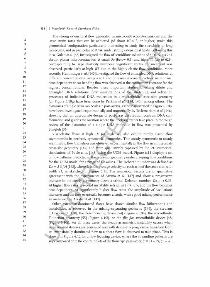
1

2

3

4

5

6

7

8

9

10

11

12

13

14

15

16

17

18

19

20

21

22

23

24

25

26

27

28

29

30

31

32

33

34

35

36

37

38

39

40

41

42

43

44

45

The strong extensional flow generated in microcontraction/expansions and thelarge strain rates that can be achieved (of about 105 s�1, or higher) make thisgeometrical configuration particularly interesting to study the stretching of longmolecules, and in particular of DNA, under strong extensional fields. Following thisidea, Gulati et al. [38] investigated the flow of semidilute solutions of l-DNA in a 2 : 1abrupt planar microcontraction at small Re (below 0.1) and high Wi (up to 629),corresponding to large elasticity numbers. Significant vortex enhancement wasobserved, particularly at high Wi, due to the highly elastic flow conditions. Morerecently, Hemminger et al. [143] investigated the flow of entangled DNA solutions, atdifferent concentrations, using a 4 : 1 abrupt planar microcontraction. An unusualtime-dependent shear banding flow was observed at the contraction entrance for thehighest concentrations. Besides these important studies involving dilute andentangled DNA solutions, flow visualizations of the stretching and relaxationprocesses of individual DNA molecules in a microfluidic cross-slot geometry(cf. Figure 6.10g) have been done by Perkins et al. [144, 145], among others. Thedynamics of singleDNAmolecules in post-arrays, as those illustrated inFigure 6.10p,have been investigated experimentally and numerically by Teclemariam et al. [146],showing that an appropriate design of post-array distribution controls DNA con-formation and guides the location where the hooking events take place. A thoroughreview of the dynamics of a single DNA molecule in flow was presented byShaqfeh [36].

Viscoelastic flows at high De (or high Wi) also exhibit purely elastic flowasymmetries in perfectly symmetric geometries. This steady symmetric to steadyasymmetric flow transition was observed experimentally in the flow in a microscalecross-slot geometry [147] and were qualitatively captured by the 2D numericalsimulations of Poole et al. [148] using the UCM model. Figure 6.11 displays a setof flow patterns predicted in the cross-slot geometry under creeping flow conditionsfor the UCM model for a range of De values. The Deborah number was defined asDe ¼ lU=H [148], whereU is the average velocity on each arm of the cross-slot, withwidth H, as sketched in Figure 6.11. The numerical results are in qualitativeagreement with the experiments of Arratia et al. [147] and show a progressiveincrease in the steady asymmetry above a critical Deborah number, Decrit � 0:31.At higher flow rates, a second instability sets in, at De � 0:5, and the flow becomestime-dependent. At significantly higher flow rates, the amplitude of oscillationsincreases and the flow eventually becomes chaotic, with a good mixing performanceas measured by Arratia et al. [147].

Other extension-dominated flows have shown similar flow bifurcations andinstabilities, as observed in the mixing–separating geometry [149], the six-arms3D cross-slot [150], the flow-focusing device [54] (Figure 6.10h), the microfluidicT-junction geometry [55] (Figure 6.10i), or the flip–flop microfluidic device [48](Figure 6.10j). For all these cases, the steady asymmetric instability occurs whenlarge normal stresses are generated and with its onset a progressive transition froman extensionally dominated flow to a shear flow is observed to take place. This isshown in Figure 6.12 for a flow-focusing device, where the streamline patterns aresuperimposed onto the contour plots of theflow-type parameter, j � ð1�RÞ=ð1þRÞ;

158j 6 Microfluidic Flows of Viscoelastic Fluids

1

2

3

4

5

6

7

8

9

10

11

12

13

14

15

16

17

18

19

20

21

22

23

24

25

26

27

28

29

30

31

32

33

34

35

36

37

38

39

40

41

42

43

44

45

with R ¼ trðW2Þ=trðD2Þ, where W is the relative rate of rotation tensor and D is thestrain-rate tensor [151]. This invariant is illustrated in Figure 6.12 and varies fromj ¼ �1, corresponding to solid-like rotation flow, up to j ¼ 1, corresponding to pureextensional flow. Shear flow corresponds to j ¼ 0 and is easily identified near thewalls, and along the channels under fully developed flow conditions.

Figure 6.11 (a) Sketch of the cross-slotgeometry. Streamline patterns predicted undercreeping flow conditions for (b) a Newtonianfluid, and a UCM model at (c) De¼ 0.3 and (d)

De¼ 0.5. The contours in (b–d) represent thenormalized normal stress, tyy=ðgU=HÞ.Adapted from [148].

Figure 6.12 Extensional flow of a UCM fluid in a flow focusingmicrogeometry under creeping flowconditions. (a) Sketch of the geometry; (b) De¼ 0.3; (c) De¼ 0.34. Adapted from [54].

6.5 Passive Mixing for Viscoelastic Fluids: Purely Elastic Flow Instabilities j159

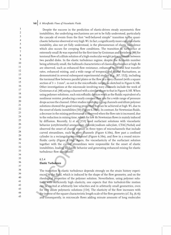
1

2

3

4

5

6

7

8

9

10

11

12

13

14

15

16

17

18

19

20

21

22

23

24

25

26

27

28

29

30

31

32

33

34

35

36

37

38

39

40

41

42

43

44

45

Despite the success in the prediction of elastic-driven steady asymmetric flowinstabilities, the underlying mechanisms are yet to be fully understood, particularlythe cascade of events from the first �well-behaved simple� transition to the quasi-chaotic behavior observed at very highWi. In fact, a significantlymore complex elasticinstability, also not yet fully understood, is the phenomenon of elastic turbulencewhich also occurs for creeping flow conditions. The transition to turbulence atextremely smallRewas reported for the first time by Groisman and Steinberg [88] fortorsionalflowof a dilute solution of a high-molecular-weight polyacrylamide betweentwo parallel disks. In the elastic turbulence regime, despite the Reynolds numberbeing arbitrarily small, the hallmark characteristics of classical turbulence at high Reare observed, such as enhanced flow resistance, enhanced mass and heat transferrates, enhanced mixing, and a wide range of temporal and spatial fluctuations, asdemonstrated in several subsequent experimental studies (e.g., [87, 152]), includingthe torsional flow between parallel plates or the flow in a wavy channel (with a squaresection of 3� 3mm2, so not in the microfluidic range), as sketched in Figure 6.10k.Other investigations at the microscale involving wavy channels include the work ofGroisman et al. [48] using a channel with a similar shape to that in Figure 6.10l.Whenusing polymer solutions, suchmicrofluidic devices work as the fluidic equivalent of anonlinear resistor, producing a nearly constant flow rate for a wide range of pressuredrops across the channel.Other studies involving zigzag channels anddilute polymersolutions showed the goodmixing properties that can be achieved at highWi, due tothe onset of elastic instabilities [50] (Figure 6.10m). In contrast, for Newtonian fluids,a decrease in themixingperformance is observedwhen theflow rate is increased, dueto the reduction inmixing time, which for lowReNewtonian flows ismainly inducedby diffusion. Recently, Li et al. [153] used surfactant solutions with viscoelasticbehavior (cetyltrimethyl ammonium chloride/sodium salicylate, CTAC/NaSal) andobserved the onset of chaotic motion in three types of microchannels that includecurved streamlines, such as wavy channels (Figure 6.10n), flow past a confinedcylinder in a rectangular microchannel (Figure 6.10o), and flow in a round micro-fluidic cavity (Figure 6.10q). Again, the viscoelasticity of the surfactant solutiontogether with the curved streamlines were responsible for the onset of elasticinstabilities, leading to chaotic behavior and generating enhanced mixing for elasticturbulence flow conditions.

6.5.4Elastic Turbulence

The transition to elastic turbulence depends strongly on the strain history experi-enced by the fluid, which is induced by the shape of the flow geometry, and on therheological properties of the polymer solution. Nevertheless, using polymer solu-tions with sufficiently high elasticity, one expects that this turbulent-like motioncan be excited at arbitrarily low velocities and in arbitrarily small geometries, evenfor very dilute polymeric solutions [154]. The elasticity of the flow increases withthe inverse of the square characteristic length scale of the flow geometry (cf. Eq. (6.4))and consequently, in microscale flows adding minute amounts of long molecules

160j 6 Microfluidic Flows of Viscoelastic Fluids

1

2

3

4

5

6

7

8

9

10

11

12

13

14

15

16

17

18

19

20

21

22

23

24

25

26

27

28

29

30

31

32

33

34

35

36

37

38

39

40

41

42

43

44

45

to the solution (on the order of 10 ppm, or above), is usually sufficient to inducenon-Newtonian behavior at large deformation rates, which are typical of microscaleflows [52, 87, 155].

So far, most of the works concerning elastic turbulence have been primarilyexperimental [87, 88, 152, 154, 156], and theoretical [155, 157]. The numericalsimulation of elastic-driven flow instabilities has been restricted to the initial phasesof flow transitions [125, 138, 148]. Only recently some preliminary attempts tosimulate the elastic turbulence regime have been successful, for simplified 2D flowarrangements, such as the periodic Kolmogorov shear flow with constant forc-ing [158, 159]. Using direct numerical simulations (DNS) and the Oldroyd-B modelto describe the fluid rheology, these authors demonstrated the occurrence of flowdestabilization induced by the elastic forces due to the dynamics of polymermolecules in the solution. At large Wi, the basic phenomenology found in exper-imental studies of elastic turbulence was reproduced in this idealized geometricalconfiguration, with the appearance of coherent structures in the form of �elasticwaves� [159]. Despite the use of an idealized geometrical configuration with thecorresponding limitations, namely the assumptionof 2Dflow,Berti andBoffetta [159]demonstrated that the use of simple viscoelastic models, such as the Oldroyd-Bconstitutive equation, can capture the essential features of elastic turbulence,opening a window to more realistic simulations using real 3D microfluidic flowgeometries and more adequate constitutive equations.

Much more needs to be investigated regarding the progressive transitionsto elastic turbulence and this must be accomplished experimentally, using fluidsof well-controlled rheology, and complemented with computational and theoreticalstudies for better insight of the complex underlying mechanisms of flow instabil-ities. Although there are important similarities between inertial and elasticturbulence, this does not imply that the underlying physical mechanism is thesame in both cases. Indeed, elastic turbulence is accompanied by significantstretching of the polymer molecules, which is the main cause of the observedincrease in the elastic normal stresses and the inherent increase in flow resistance,a ubiquitous characteristic of turbulence. The stretching of the molecular chainsleads to a strong increase in flow resistance due to the increase in the extensionalviscosity, a characteristic of long macromolecules in extensional flow [45], verymuch like the production of large Reynolds stresses in inertial turbulence ofNewtonian fluids, but contrasting with the severe damping of the same Reynoldsstresses that accompany polymer-induced drag reduction in high Re inertialturbulence. Understanding the nature and mechanisms that lead to elastic turbu-lence will have important practical applications, either for enhancing mixingand/or heat and mass transfer rates at the microscale, or for allowing the operationof extrusion processes at higher throughputs, by minimizing the driving forcesthat lead to the onset of flow instabilities. Additionally, understanding the drivingmechanisms of elastic turbulence and comparison with classical inertial-driventurbulence of Newtonian fluids may allow us to obtain further insights into thedriving mechanisms of inertial turbulence in Newtonian and in viscoelasticfluid flows.

6.5 Passive Mixing for Viscoelastic Fluids: Purely Elastic Flow Instabilities j161

1

2

3

4

5

6

7

8

9

10

11

12

13

14

15

16

17

18

19

20

21

22

23

24

25

26

27

28

29

30

31

32

33

34

35

36

37

38

39

40

41

42

43

44

45

6.6Other Forcing Methods

The previous section discussed instabilities at high Wi flows of complex fluidsdriven by a pressure gradient. Here we briefly describe important works that useelectrokinetic forcing to promote complex fluid flow, with emphasis on EO andelectrophoresis. EOF are important in the context of viscoelastic fluids, includingthe development of instabilities and their possible application in micromixingenhancement. To finalize this chapter, electrophoresis is also considered, not in theframework of mixing, but rather because of its importance in the limiting case ofthe manipulation and separation of individual macromolecules, and of its closelink with EO.

6.6.1Electro-Osmosis

Currently, about 90% of microfluidic devices operate by either pressure-driven orEOF forcing, essentially due to their versatility and simplicity of operation [160]. PDFare still leading the number of applications of microfluidics; however as the size ofthe microchannels is further reduced, say to dimensions below around 10 mm,forcing by pressure becomes particularly inefficient due to the significant increase inviscous losses [160]. In contrast, for this range of dimensions EO becomes aparticularly convenient and efficient way of promoting flow in microfluidic devices,as long as the fluid has ions. A major disadvantage of EOF is the strong electricgradients that typically need to be applied to promote the flow at average velocitiesabove 1mms�1. This limitation can be circumvented by further miniaturization,thusmaking EOFmore efficient as the size is reduced, with important applications innanofluidics where smaller electrical potentials are sufficient to promote the flow.A thorough discussion on the advantages and disadvantages of PDF and EOF ispresented in [160].

Rigorous modeling of EOF in microchannels has been the subject of severalstudies, particularly for Newtonian fluids. A thorough review with various appli-cations of EO is presented in [58, 161]. Exact analytical solutions have been derivedunder fully developed flow conditions for Newtonian fluids, as described byAfonso et al. [162]. Newtonian fluid flow in complex geometries has been modeledin several works, and accurate results have been obtained for different applications.Of particular interest are electrokinetic instabilities (EKI) that arise under highelectric fields in the presence of electrical conductivity gradients. Electrokineticflows of Newtonian fluids become unstable when electroviscous advection of con-ductivity fields dominates over dissipation through viscosity and molecular diffu-sion [163, 164]. Likewise, EKI can be triggered using time-periodic fields, asdemonstrated by Shin et al. [165] using a flow-focusing device (Figure 6.10h).

Surface patterning with different materials has been exploited to generateregions with different zeta potentials, and chaotic mixing in EOF can be driven byspatiotemporal surface charge modulation [166]. Other examples of nonlinear

162j 6 Microfluidic Flows of Viscoelastic Fluids

1

2

3

4

5

6

7

8

9

10

11

12

13

14

15

16

17

18

19

20

21

22

23

24

25

26

27

28

29

30

31

32

33

34

35

36

37

38

39

40

41

42

43

44

45

electrokinetic phenomena with great potential in microfluidics mixing and pump-ing are induced-charge electro-osmosis (ICEO) and AC electro-osmosis (ACEO), asreviewed by Bazant and Squires [167].

In contrast, EOF of complex fluids are still poorly studied, except for fullydeveloped flows between parallel plates and in a circular tube, thus constitutinga fertile ground for research. The theoretical study of EO flows of non-Newtonianfluids is recent and the preliminary works considered GNF, such as the power-lawmodel [168, 169]). Berli and Olivares [170] considered the existence of a small walllayer depleted of additives (the skimming layer), in which the fluid behaves as aNewtonian fluid, and the non-Newtonian behavior is restricted to the electricallyneutral region outside the EDL. More recently, the theoretical analysis of EOflows was extended to viscoelastic fluids by Park and Lee [171], who derived theHelmholtz–Smoluchowski velocity for pure EOF of PTT fluids in rectangularchannels and provided a simple numerical procedure for its calculation. Afonsoet al. [162] considered the PTT and FENE-P constitutive equations, and derivedanalytical expressions for fully developedflowbetweenparallel plates and in a circularpipe, under combined pressure and electrokinetic forcings. This analysis wasextended by Afonso et al. [172] to consider different zeta potentials on both walls,whereas Sousa et al. [173] considered the existence of a skimming layer near the walldepleted of polymer molecules.

EOF of polymer solutions have also been studied experimentally in simplegeometries. Bello et al. [174] investigated the flow of polymer solutions in capillaries,and observed a progressively suppressed EOF, suggesting a dynamic coating ofthe polymer molecules onto the capillary wall. Baumler et al. [175] and Chang andTsao [176] observed drag reduction in EOF of polymer solutions, due to polymerdepletion in theEDL,which leads to a reduction in shear viscositywith correspondingenhancement of the measured Helmholtz–Smoluchowski velocity.

High Weissenberg number flows are prone to purely elastic instabilities, asdiscussed in the previous section. EOF of polymer solutions are no exception, andDhinakaran et al. [118] predicted a constitutive-related instability for EO flowbetween parallel plates of PTT fluids, when the shear rate exceeds a critical value.Purely elastic instabilities can also be generated in EOflows, and such electroelasticinstabilities were recently observed experimentally in a microfluidic channelconsisting of a series of 2 : 1 sudden contraction/expansions (Figure 6.10f), usingdilute viscoelastic PAA solutions [177, 178]. EOF are an excellent platform togenerate strong extensional flows because shear effects are typically circumscribedto the EDL region. The experimental results of Bryce and Freeman [177, 178]suggest that the electroelastic instability occurs for flow conditions correspondingto the coil–stretch transition, without the observation of a dominant frequency ofthe flow, an indication of chaotic-like behavior. Despite this unstable behavior, themixing rates found were smaller than those observed in polymer-free solutions,with diffusion appearing to be the dominant mixing mechanism [177]. This is asurprising result, and further investigations of electroelastic instabilities arerequired to enlighten the mechanism of purely elastic instabilities and mixing inmicrofluidic EO flows of polymer solutions.

6.6 Other Forcing Methods j163

1

2

3

4

5

6

7

8

9

10

11

12

13

14

15

16

17

18

19

20

21

22

23

24

25

26

27

28

29

30

31

32

33

34

35

36

37

38

39

40

41

42

43

44

45

6.6.2Electrophoresis

In many ways, DNA can be considered as an ideal model polymer. It is naturallymonodisperse, large enough to be imaged in a microscope using fluorescencetechniques, and the relaxation time is typically of the order of seconds [179]. DNAis a polyelectrolyte, making it easy to be manipulated through electrophoresis byapplying electric fields. We note, however, that the (micro)fluidic channels usedusually have charged surfaces, which also induce a global transport through EO,unless special treatments are applied to the surfaces to minimize electro-osmotictransport [180].

In a strict sense, electrophoresis is usually not included in the field of rheology.However, since it involves deformation and flow of matter, albeit in a single mole-cule framework, this tacit distinction is becoming obsolete, with experimentsusing biopolymers progressively creating an important influence on rheology [179].Likewise, some tools developed for microrheology are expected to be increasinglyused in the manipulation of single DNA molecules. A growing interaction betweenrheology and biophysics is leading to important insights into the flow properties ofpolymers and biomolecules [181]. Electrophoresis of macromolecules has severalapplications in molecular biology, including the transport, separation, or elongationat the molecular level, with important applications in biotechnology and medicine,with DNA sequencing being one of the most prominent. A recent review of electro-phoretic microfluidic separation techniques was presented by Wu et al. [182],summarizing important milestones in the separation of small molecules, DNA,and proteins.

Specificmicrofluidic devices have been proposed and optimized in order to studyindividual molecules, and DNA in particular. Stretching of DNAmolecules is a keytechnology in emerging DNA-mapping devices such as direct linear analysis [183],and single-molecule studies of DNA have expanded our knowledge on the funda-mentals of polymer physics. Additionally, understanding the response of individualpolymers at themolecular level can provide valuable information to developmodelsapplicable to entangled systems. Electrophoresis stretching and relaxation of DNAmolecules have been undertaken in several flow configurations that promote astrong extensional field, such as hyperbolic contractions, cross–slot, and T-junctionarrangements. Juang et al. [184] used a cross-slot microfluidic channel to induce afairly homogeneous 2D elongational flow, allowing the determination of theamount of DNA stretching. Kim and Doyle [183] used hyperbolic contractions,which generate a nearly constant strain rate, with additional lateral streams toenhance DNA stretching. Balducci and Doyle [185] also used hyperbolic contrac-tions, but included an obstacle array upstream of the contraction region forconformational preconditioning, leading to an increase in the average deformationof the DNA molecule in the contraction. Tang and Doyle [186] proposed amicrofluidic T-shaped channel which can trap and significantly stretch singleDNA molecules using electrophoresis, without requiring any special end functio-nalization to trap the DNA molecule.

164j 6 Microfluidic Flows of Viscoelastic Fluids

1

2

3

4

5

6

7

8

9

10

11

12

13

14

15

16

17

18

19

20

21

22

23

24

25

26

27

28

29

30

31

32

33

34

35

36

37

38

39

40

41

42

43

44

45

The relaxation process of DNA is also of interest as it allows for the determinationof the molecular relaxation time, which is an important parameter for the charac-terization of DNA dynamics as shown in several experimental studies [187–189].

6.7Conclusions and Perspectives

Flow systems built aroundmicrofluidics are becoming increasingly popular in awiderange of industrial applications dealing with both gas and liquids. They associate lowproduction costs with low power consumption and waste reduction, allow for easyintegration with electronics toward the lab-on-chip devices, but require demandingmanufacturing facilities and highly efficient signal detection systems. Many of theirapplications are in biotechnology and in health related areas, where the liquids aremade of complex structures and macromolecules that impart nonlinear rheologicalbehavior and in particular viscoelasticity. Since microscale flows are characterizedby high surface-to-volume ratios, the flow dynamics is significantly affected byfluid rheology and other physical phenomena, such as surface tension, in compar-ison with macroscale flows. In particular, the time scale of the flows, tf � L=U,decreases significantly to become much smaller than (or at least on the order of) therelaxation time of the fluid structures, keeping the flowReynolds number small. As aconsequence, microscale flows of complex fluids are characterized by large elasticeffects in comparison to the corresponding Newtonian flows and both exhibit largeratios of viscous to inertial forces, in contrast to the corresponding macroscale flowsdominated by inertia.

The large elastic effects found in microfluidic flows of complex fluids allow forenhanced mixing due to purely elastic instabilities, which are a consequence of thenonlinear nature of the corresponding terms of the rheological constitutive equation.In fact, the onset of elastic instabilities has been found to take place over a wide rangeof flow types (flows dominated by extension or shear, as well as flows having mixedkinematics), whenever there are large normal stresses of elastic origin coupled withstreamline curvature. The dynamics of these instabilities, which exist even in thelimit of creeping flow, do have some resemblance to inertial instabilities found inhigh Reynolds number flows of Newtonian fluids, in the sense of a progressivecascade of instabilities from simple transitions between steady flows to transitions toperiodic unsteady and subsequently chaotic flows leading eventually to elasticturbulence, where the unstable flow structures exist over a continuous wide rangeof length and time scales. The path of these transitions is only now being discoveredand remains an active topic of research. The onset of elastic turbulence in regions ofparallel shear flow is currently particularly challenging.

The presence of macromolecules in microscale flow systems thus allows forenhanced mixing in low Reynolds number flows via elasticity-driven instabilities.These not only exist in pressure-gradient driven flows, but also for electrically drivenflows, which are potentially very useful given their ease of implementation at thesescales. The combination of EO with viscoelasticity is a new topic of research, where

6.7 Conclusions and Perspectives j165

1

2

3

4

5

6

7

8

9

10

11

12

13

14

15

16

17

18

19

20

21

22

23

24

25

26

27

28

29

30

31

32

33

34

35

36

37

38

39

40

41

42

43

44

45

most things remain to be done and it suffices to think here that it is not only directbut also alternate current that has to be considered. Additionally, electrokineticeffects can be combined with surface patterning, which can also be used to enhanceother surface phenomena, such as the generation of surface tension gradients. Theircombination with complex fluids is in its infancy and is certainly worth exploring tofind possible and unexpected flow features and applications.

Acknowledgments

The authors acknowledge funding by FEDER and Fundac~ao para a Ciencia e aTecnologia over the last 6 years through projects REEQ/262/EME/2005, REEQ/928/EME/2005, POCI/EME/59338/2004, PTDC/EME-MFE/70186/2006, PTDC/EQU-FTT/70727/2006, and PTDC/EQU-FTT/71800/2006.

References

1 Squires, T.M. and Quake, S.R. (2005)Microfluidics: Fluid physics at thenanoliter scale.Reviews ofModern Physics,77, 977–1026.

2 Whitesides, G.M. (2006) The origins andthe future of microfluidics. Nature, 442,368–373.

3 Saville, D.A. (1977) Electrokinetic effectswith small particles. Annual Review ofFluid Mechanics, 9, 321–337.

4 Probstein, R.F. (2003) PhysicochemicalHydrodynamics, an Introduction, 2nd edn,Wiley-Interscience, Hoboken, NJ.

5 Gad-el-Hak, M.G. (2002) The MEMSHandbook, CRC Press, Boca Raton, FL.

6 Bruus,H. (2008)TheoreticalMicrofluidics,Oxford Master Series in Condensed MatterPhysics, Oxford University Press, Oxford,UK.

7 Ajdari, A. (2000) Pumping liquids usingasymmetric electrode arrays. PhysicalReview E, 61, R45–R48.

8 Bazant, M.Z. and Squires, T.M. (2004)Induced-charge electrokineticphenomena: Theory and microfluidicapplications. Physical Review Letters, 92,066101.

9 Stone,H.A., Stroock, A.D., and Ajdari, A.(2004) Engineering flows in smalldevices: microfluidics toward lab-on-a-chip. Annual Review of Fluid Mechanics,36, 381–411.

10 Laser, D.J. and Santiago, J.G. (2004) Areview of micropumps. Journal ofMicromechanics and Microengineering,14, R35–R64.

11 Stone, H.A. (2009) Microfluidics, tuned-in flow control. Nature Physics, 5,178–179.

12 Brody, J.P., Kamholz, A.E., and Yager, P.(1997) Prominent microscopic effects inmicrofabricated fluidic analysis systems.Micro- and Nanofabricated Electro-Optical Mechanical Systems forBiomedical and EnvironmentalApplications, Proceedings of, 2978 pp.103–110.

13 Hatch, A., Kamholz, A.E., Hawkins, K.R.,Munson, M.S., Schilling, E.A., Weigl,B.H., and Yager, P. (2001) A rapiddiffusion immunoassay in a T-sensor.Nature Biotechnology, 19, 461–465.

14 Dendukuri, D., Tsoi, K., Hatton, T.A.,and Doyle, P.S. (2005) Controlledsynthesis of nonspherical microparticlesusing microfluidics. Langmuir, 21,2113–2116.

15 Nguyen, N.-T. (2008) Micromixers:Fundamentals, Design and Fabrication,William Andrew, Norwich, NY.

16 Sia, S.K. and Whitesides, G.M. (2003)Microfluidic devices fabricated in poly(dimethylsiloxane) for biological studies.Electrophoresis, 24, 3563–3576.

166j 6 Microfluidic Flows of Viscoelastic Fluids

1

2

3

4

5

6

7

8

9

10

11

12

13

14

15

16

17

18

19

20

21

22

23

24

25

26

27

28

29

30

31

32

33

34

35

36

37

38

39

40

41

42

43

44

45

17 Pittet, P., Lu, G.N., Galvan, J.M.,Ferrigno, R., Stephan, K., Blum, L.J., andLeca-Bouvier, B. (2008) A novel low-costapproach of implementingelectrochemiluminescence detection formicrofluidic analytical systems.MaterialsScience & Engineering C-Biomimetic andSupramolecular Systems, 28, 891–895.

18 Kallio, P. and Kuncova, J. (2004)Microfluidics. Technology Review, 158,2004.

19 Nguyen, N.T. and Wu, Z.G. (2005)Micromixers – a review. Journal ofMicromechanics and Microengineering,15, R1–R16.

20 Oh, K.W. and Ahn, C.H. (2006) A reviewof microvalves. Journal of Micromechanicsand Microengineering, 16, R13–R39.

21 Quake, S.R. and Scherer, A. (2000) Frommicro- to nanofabrication with softmaterials. Science, 290, 1536–1540.

22 Ng, J.M.K., Gitlin, I., Stroock, A.D., andWhitesides, G.M. (2002)Components forintegrated poly(dimethylsiloxane)microfluidic systems. Electrophoresis,23, 3461–3473.

23 Marrian, C.R.K. and Tennant, D.M.(2003) Nanofabrication. Journal ofVacuum Science & Technology A – VacuumSurfaces and Films, 21, S207–S215.

24 Bayraktar, T. and Pidugu, S.B. (2006)Characterization of liquid flows inmicrofluidic systems. InternationalJournal of Heat and Mass Transfer,49, 815–824.

25 Whitesides, G.M. and Stroock, A.D.(2001) Flexible methods formicrofluidics. Physics Today, 54, 42–48.

26 Thorsen, T., Roberts, R.W., Arnold, F.H.,and Quake, S.R. (2001) Dynamic patternformation in a vesicle-generatingmicrofluidic device. Physical ReviewLetters, 86, 4163–4166.

27 Anna, S.L., Bontoux, N., and Stone, H.A.(2003) Formation of dispersions using�flow focusing� in microchannels.Applied Physics Letters, 82, 364–366.

28 Yang, T.L., Jung, S.Y., Mao, H.B., andCremer, P.S. (2001) Fabrication ofphospholipid bilayer-coatedmicrochannels for on-chipimmunoassays. Analytical Chemistry,73, 165–169.

29 Fu, A.Y., Spence, C., Scherer, A., Arnold,F.H., and Quake, S.R. (1999) Amicrofabricated fluorescence-activatedcell sorter. Nature Biotechnology, 17,1109–1111.

30 Sohn, L.L., Saleh, O.A., Facer, G.R.,Beavis, A.J., Allan, R.S., and Notterman,D.A. (2000) Capacitance cytometry:Measuring biological cells one by one.Proceedings of the National Academy ofSciences of the United States of America,97, 10687–10690.

31 Chiu, D.T., Jeon, N.L., Huang, S.,Kane, R.S.,Wargo,C.J., Choi, I.S., Ingber,D.E., and Whitesides, G.M. (2000)Patterned deposition of cells andproteins onto surfaces by using three-dimensional microfluidic systems.Proceedings of the National Academy ofSciences of the United States of America, 97,2408–2413.

32 Li, J.J., Kelly, J.F., Chemushevich, I.,Harrison, D.J., and Thibault, P. (2000)Separation and identification of peptidesfrom gel-isolated membrane proteinsusing a microfabricated device forcombined capillary electrophoresis/nanoelectrospray mass spectrometry.Analytical Chemistry, 72, 599–609.

33 Beebe, D.J., Mensing, G.A., and Walker,G.M. (2002) Physics and applications ofmicrofluidics in biology.Annual Review ofBiomedical Engineering, 4, 261–286.

34 Zare, R.N. and Kim, S. (2010)Microfluidic platforms for single-cellanalysis. Annual Review of BiomedicalEngineering, 12, 187–201.

35 Tegenfeldt, J.O., Prinz, C., Cao, H.,Huang, R.L., Austin, R.H., Chou, S.Y.,Cox, E.C., and Sturm, J.C. (2004) Micro-and nanofluidics for DNA analysis.Analytical and Bioanalytical Chemistry,378, 1678–1692.

36 Shaqfeh, E.S.G. (2005) The dynamics ofsingle-molecule DNA in flow. Journal ofNon-Newtonian Fluid Mechanics, 130,1–28.

37 Randall, G.C., Schultz, K.M., and Doyle,P.S. (2006) Methods toelectrophoretically stretch DNA:Microcontractions, gels, and hybrid gel-microcontraction devices. Lab on a Chip,6, 516–525.

References j167

1

2

3

4

5

6

7

8

9

10

11

12

13

14

15

16

17

18

19

20

21

22

23

24

25

26

27

28

29

30

31

32

33

34

35

36

37

38

39

40

41

42

43

44

45

38 Gulati, S., Muller, S.J., and Liepmann, D.(2008) Direct measurements ofviscoelastic flows of DNA in a 2: 1abrupt planar micro-contraction. Journalof Non-Newtonian Fluid Mechanics, 155,51–66.

39 Choban, E.R., Markoski, L.J.,Wieckowski, A., and Kenis, P.J.A. (2004)Microfluidic fuel cell based on laminarflow. Journal of Power Sources, 128, 54–60.

40 Obot, N.T. (2002) Toward a betterunderstanding of friction and heat/masstransfer in microchannels – A literaturereview. Microscale ThermophysicalEngineering, 6, 155–173.

41 Hansen, C. and Quake, S.R. (2003)Microfluidics in structural biology:smaller, faster. . . better. Current Opinionin Structural Biology, 13, 538–544.

42 Gad-el-Hak, M. (2005) Liquids: The holygrail of microfluidic modeling. Physics ofFluids, 17, 100612.

43 Breussin, F. (2009) Emergingmarkets formicrofluidic applications in Life Sciencesand In-Vitro Diagnostics, EMMAReport,Yole D�evelopment SA.

44 Tabeling, P. (2005) Introduction toMicrofluidics, Oxford University Press,Oxford.

45 Bird, R.B., Armstrong, R.C., andHassager,O. (1987)Dynamics of PolymericLiquids. Volume 1: Fluid Mechanics, Wiley,New York.

46 Larson, R.G. (1999) The Structure andRheology of Complex Fluids, OxfordUniversity Press, Oxford.

47 Dealy, J.M. (2010) Weissenberg andDeborah numbers – Their definition anduse. Rheology Bulletin, 79, 14–18.

48 Groisman, A., Enzelberger, M., andQuake, S.R. (2003) Microfluidic memoryand control devices. Science, 300,955–958.

49 Groisman, A. and Quake, S.R. (2004) Amicrofluidic rectifier: anisotropic flowresistance at low Reynolds numbers.Physical Review Letters, 92, 094501-1–094501-4.

50 Pathak, J.A., Ross, D., and Migler, K.B.(2004) Elastic flow instability,curved streamlines, and mixing inmicrofluidic flows. Physics of Fluids, 16,4028-1–4028-7.

51 Rodd, L.E., Scott, T.P., Boger, D.V.,Cooper-White, J.J., and McKinley, G.H.(2005) The inertio-elastic planar entryflow of low-viscosity elastic fluids inmicro-fabricated geometries. Journal ofNon-Newtonian Fluid Mechanics, 129,1–22.

52 Sousa, P.C., Pinho, F.T., Oliveira,M.S.N.,and Alves, M.A. (2010) Efficientmicrofluidic rectifiers for viscoelasticfluid flow. Journal of Non-Newtonian FluidMechanics, 165, 652–671.

53 Gan, H.Y., Lam, Y.C., and Nguyen, N.T.(2006) Polymer-based device for efficientmixing of viscoelastic fluids. AppliedPhysics Letters, 88, 224103.

54 Oliveira, M.S.N., Pinho, F.T., Poole, R.J.,Oliveira, P.J., and Alves, M.A. (2009)Purely-elastic flow asymmetries inflow-focusing devices. Journal ofNon-Newtonian Fluid Mechanics, 160,31–39.

55 Soulages, J., Oliveira, M.S.N., Sousa,P.C., Alves, M.A., and McKinley, G.H.(2009) Investigating the stability ofviscoelastic stagnation flows in T-shapedmicrochannels. Journal of Non-NewtonianFluid Mechanics, 163, 9–24.

56 Batchelor, G.K. (2000) An Introduction toFluid Dynamics, Cambridge UniversityPress, Cambridge, UK; New York, NY.

57 Nguyen, N.-T. and Wereley, S.T. (2006)Fundamentals and Applications ofMicrofluidics, 2nd edn, Artech House,Norwood.

58 Karniadakis, G., Beskok, A., and Aluru,N. (2005) Microflows and nanoflows.Fundamentals and Simulation,Interdisciplinary Applied MathematicsSeries, vol. 29, Springer, Berlin.

59 Koo, J.M. and Kleinstreuer, C. (2003)Liquid flow in microchannels:experimental observations andcomputational analyses of microfluidicseffects. Journal of Micromechanics andMicroengineering, 13, 568–579.

60 Sharp, K.V. and Adrian, R.J. (2004)Transition from laminar to turbulentflowin liquid filledmicrotubes. Exp Fluids, 36,741–747.

61 Oliveira,M.S.N., Alves,M.A., Pinho, F.T.,and McKinley, G.H. (2007) Viscous flowthrough microfabricated hyperbolic

168j 6 Microfluidic Flows of Viscoelastic Fluids

1

2

3

4

5

6

7

8

9

10

11

12

13

14

15

16

17

18

19

20

21

22

23

24

25

26

27

28

29

30

31

32

33

34

35

36

37

38

39

40

41

42

43

44

45

contractions. Experiments in Fluids, 43,437–451.

62 Oliveira, M.S.N., Rodd, L.E.,McKinley, G.H., and Alves, M.A. (2008)Simulations of extensional flow inmicrorheometric devices. MicrofluidNanofluid, 5, 809–826.

63 Pit, R., Hervet, H., and Leger, L. (2000)Direct experimental evidence of slip inhexadecane: Solid interfaces. PhysicalReview Letters, 85, 980–983.

64 Barrat, J.L. and Bocquet, L. (1999) Largeslip effect at a nonwetting fluid-solidinterface. Physical Review Letters, 82,4671–4674.

65 Colin, S. (2005) Rarefaction andcompressibility effects on steady andtransient gas flows in microchannels.Microfluid Nanofluid, 1, 268–279.

66 Pipe, C.J. and McKinley, G.H.(2009) Microfluidic rheometry.Mechanics Research Communications,36, 110–120.

67 Ottino, J.M. and Wiggins, S. (2004)Applied physics – Designing optimalmicromixers. Science, 305, 485–486.

68 Wang, H.Z., Iovenitti, P., Harvey, E., andMasood, S. (2002) Optimizing layout ofobstacles for enhanced mixing mmicrochannels. Smart Materials &Structures, 11, 662–667.

69 Brody, J.P., Yager, P., Goldstein, R.E., andAustin, RH. (1996) Biotechnology at lowReynolds numbers. Biophysical Journal,71, 3430–3441.

70 Ottino, J.M. (2004) The Kinematicsof Mixing: Stretching, Chaos, andTransport, Cambridge University Press,Cambridge, UK.

71 Coleman, J.T. and Sinton, D. (2005) Asequential-injection microfluidic mixingstrategy. Microfluid Nanofluid, 1,319–327.

72 Glasgow, I. and Aubry, N. (2003)Enhancement of microfluidic mixingusing time pulsing. Lab on a Chip, 3,114–120.

73 Deshmukh, A.A., Liepmann, D., andPisano, A.P. (2000) Continuousmicromixer with pulsatile micropumps.Technical Digest of the IEEE Solid StateSensor and Actuator Workshop (HiltonNead Island, SC) 73–76.

74 El Moctar, A.O., Aubry, N., and Batton, J.(2003) Electro-hydrodynamic micro-fluidic mixer. Lab on a Chip, 3, 273–280.

75 Bau, H.H., Zhong, J., and Yi, M. (2001) Aminute magneto hydro dynamic (MHD)mixer. Sensors and Actuators B: Chemical,79, 207–215.

76 Qian, S. and Bau, H.H. (2009) Magneto-hydrodynamics based microfluidics.Mechanics Research Communications, 36,10–21.

77 Yang, Z., Goto, H., Matsumoto, M., andMaeda, R. (2000) Active micromixer formicrofluidic systems using lead-zirconate-titanate (PZT)-generatedultrasonic vibration. Electrophoresis, 21,116–119.

78 Yang, Z., Matsumoto, S., Goto, H.,Matsumoto, M., and Maeda, R. (2001)Ultrasonic micromixer for microfluidicsystems. Sensor Actuators A – Phys, 93,266–272.

79 Hessel, V., Lowe, H., and Schonfeld, F.(2005) Micromixers – a review on passiveand active mixing principles. ChemicalEngineering Science, 60, 2479–2501.

80 Aref, H. (1984) Stirring by chaoticadvection. Journal of Fluid Mechanics,143, 1–21.

81 Stroock, A.D., Dertinger, S.K.W., Ajdari,A., Mezic, I., Stone, H.A., andWhitesides, G.M. (2002) Chaotic mixerformicrochannels.Science, 295, 647–651.

82 Gleeson, J.P. (2005) Transientmicromixing: Examples of laminar andchaotic stirring. Physics of Fluids, 17,100614.

83 Tadmor, Z. and Gogos, C.G. (2006)Principles of Polymer Processing, 2nd edn,Wiley-Interscience, Hoboken, NJ.

84 Oliveira, M.S.N., Pinho, F.T., and Alves,M.A. (2008) Extensional effects inviscoelastic fluid flow through a micro-scale double cross-slot. XvthInternational Congress onRheology– theSociety of Rheology 80th AnnualMeeting, Pts 1 and 2, 1027, pp. 982–984.

85 Townsend, P., Walters, K., andWaterhouse, W.M. (1976) Secondaryflows in pipes of square cross-section andmeasurement of 2nd normal stressdifference. Journal of Non-NewtonianFluid Mechanics, 1, 107–123.

References j169

1

2

3

4

5

6

7

8

9

10

11

12

13

14

15

16

17

18

19

20

21

22

23

24

25

26

27

28

29

30

31

32

33

34

35

36

37

38

39

40

41

42

43

44

45

86 Pakdel, P. and McKinley, G.H. (1996)Elastic instability and curved streamlines.Physical Review Letters, 77, 2459–2462.

87 Groisman, A. and Steinberg, V. (2004)Elastic turbulence in curvilinear flows ofpolymer solutions.New Journal of Physics,6–29, 1–48.

88 Groisman, A. and Steinberg, V. (2000)Elastic turbulence in a polymer solutionflow. Nature, 405, 53–55.

89 Whorlow, R.W. (1992) RheologicalTechniques, 2nd edn, Ellis HorwoodSeries in Physics and Its Applications,London.

90 Walters, K. (1975) Rheometry, Chapmanand Hall, London.

91 Chen, D.C.-H. (1986) Yield stress: Atime-dependent property and how tomeasure it. Rheologica Acta, 25, 542–554.

92 Nguyen, Q.D. and Boger, D.V. (1992)Measuring the flow properties of yieldstress fluids. Annual Review of FluidMechanics, 24, 47–88.

93 Barnes, H.A. and Walters, K. (1985) Theyield stress myth? Rheologica Acta, 24,323–326.

94 Barnes, H.A. (1995) A review of the slip(wall depletion) of polymer solutions,emulsions and particle suspensions inviscometers: its cause, character andcure. Journal of Non-Newtonian FluidMechanics, 56, 221–251.

95 Barnes, H.A. (1999) The yield stress – areview or �pantarei�– everything flows?Journal of Non-Newtonian FluidMechanics, 81, 133–178.

96 Barnes, H.A., Hutton, J.F., and Walters,K. (1989) An Introduction to Rheology,Elsevier, Amsterdam.

97 Alves,M.A., Pinho, F.T., andOliveira, P.J.(2005) Visualizations of Boger fluid flowsin a 4:1 square–square contraction.AICHE Journal, 51, 2908–2922.

98 Rodd, L.E., Scott, T.P., Cooper-White, J.J.,and McKinley, G.H. (2005) Capillarybreakup rheometry for low viscosityelastic fluids. Applied Rheology, 15, 12–27.

99 Tirtaatmadja, V. and Sridhar, T. (1993) Afilament stretching device formeasurement of extensional viscosity.Journal of Rheology, 37, 1081–1102.

100 McKinley, G.H. and Sridhar, T. (2002)Filament-stretching rheometry of

complex fluids. Annual Review of FluidMechanics, 34, 375–415.

101 Sentmanat,M.L. (2003)A novel device forcharacterizing polymer flows in uniaxialextension. SPE, ANTEC Proceedings, pp.992–996.

102 Lielens, G., Keunings, R., and Legat, V.(1999) The FENE-L and FENE-LS closureapproximations to the kinetic theory offinitely extensible dumbbells. Journal ofNon-Newtonian Fluid Mechanics, 87,179–196.

103 Tanner, R.I. (2000) EngineeeringRheology, 2nd edn, Oxford Eng. ScienceSeries 52, Oxford University Press,New York.

104 Ewoldt, R.H., Hosoi, A.E., and McKinley,G.H. (2008) New measures forcharacterizing nonlinear viscoelasticity inlarge amplitude oscillatory shear. Journalof Rheology, 35 (4), 647–685.

105 Beris, A.N. and Edwards, B.J. (1994)Thermodynamics of Flowing Systems,Oxford Engineering Science Series 36,Oxford Science Publications, New York.

106 Wapperom, P. (1995) Nonisothermalflows of viscoelastic fluids.Thermodynamics, analysis andnumerics. PhD thesis. TechnicalUniversity of Delft, Holland.

107 Wapperom, P. and Hulsen, M.A. (1998)Thermodynamics of viscoelastic fluids:the temperature equation. Journal ofRheology, 42, 999–1019.

108 N�obrega, J.M., Pinho, F.T., Oliveira, P.J.,and Carneiro, O.S. (2004) Accounting fortemperature-dependent properties inviscoelastic duct flows. InternationalJournal of Heat and Mass Transfer, 47,1141–1158.

109 Bird, R.B., Armstrong, R.C., andHassager, O. (1987)Dynamics of PolymericLiquids. Volume 2: Kinetic Theory, Wiley,New York.

110 Bird, R.B., Stewart, W.E., and Lightfoot,E.N. (2002) Transport Phenomena, 2ndedn, John Wiley & Sons Inc., New York.

111 Astarita, G. and Marrucci, G. (1974)Principles of Non-Newtonian FluidMechanics, McGraw-Hill, London, NewYork.

112 Ferry, J.D. (1981) Viscoelastic Properties ofPolymers, 2nd edn, JohnWiley, New York.

170j 6 Microfluidic Flows of Viscoelastic Fluids

1

2

3

4

5

6

7

8

9

10

11

12

13

14

15

16

17

18

19

20

21

22

23

24

25

26

27

28

29

30

31

32

33

34

35

36

37

38

39

40

41

42

43

44

45

113 Wapperom, P.,Hulsen,M.A., and van derZanden, J.P.P.M. (1998) A numericalmethod for steady and nonisothermalviscoelastic fluid flow for high Deborahand P�eclet numbers. Rheologica Acta, 37,73–88.

114 Chilcott, M.D. and Rallison, J.M. (1988)Creeping flow of dilute polymer solutionspast cylinders and spheres. Journal ofNon-Newtonian Fluid Mechanics, 29,381–432.

115 Stokes, J.R., Graham, L.J.W., Lawson,N.J., and Boger, D.V. (2001) Swirling flowof viscoelastic fluids. Part 2: Elasticeffects. Journal of Fluid Mechanics, 429,117–153.

116 Larson, R.G. (1988)Constitutive Equationsfor Polymer Melts and Solutions,Butterworths, Boston.

117 Huilgol, R.R. and Phan-Thien, N. (1997)Fluid Mechanics of Viscoelasticity, Elsevier,Amsterdam.

118 Dhinakaran, S., Afonso, A.M., Alves,M.A., and Pinho, F.T. (2010) Steadyviscoelastic fluid flow in microchannelsunder electrokinetic forces: PTTmodel.Journal of Colloid and Interface Science,344, 513–520.

119 Bird, R.B. and Curtiss, C.F. (1998)Thermoviscoelasticity: continuum-molecular connections. Journal of Non-Newtonian Fluid Mechanics, 79, 255–259.

120 Peters, G.W.M. and Baaijens, F.P.T.(1997) Modelling of non-isothermalviscoelastic flows. Journal of Non-Newtonian Fluid Mechanics, 68, 205–224.

121 Larson, R.G., Shaqfeh, E.S.G., andMuller, S.J. (1990) A purely elasticinstability in Taylor–Couette flow. Journalof Fluid Mechanics, 218, 573–600.

122 McKinley, G.H., Pakdel, P., and €Oztekin,A. (1996) Rheological and geometricscaling of purely elastic flow instabilities.Journal of Non-Newtonian FluidMechanics, 67, 19–47.

123 Shaqfeh, E.S.G. (1996) Purely elasticinstabilities in viscometric flows.Annual Review of Fluid Mechanics, 28,129–185.

124 Pakdel, P. and McKinley, G.H. (1998)Cavity flows of elastic liquids: Purelyelastic instabilities. Physics of Fluids, 10,1058–1070.

125 Alves, M.A. and Poole, R.J. (2007)Divergent flow in contractions. Journal ofNon-Newtonian Fluid Mechanics, 144,140–148.

126 Boger, D.V. (1987) Viscoelastic flowsthrough contractions. Annual Review ofFluid Mechanics, 19, 157–182.

127 Owens, R.G. and Phillips, T.N. (2002)Computational Rheology, Imperial CollegePress, London.

128 Evans, R.E. and Walters, K. (1986) Flowcharacteristics associated with abruptchanges in geometry in the case of highlyelastic liquids. Journal of Non-NewtonianFluid Mechanics, 20, 11–29.

129 Evans, R.E. andWalters, K. (1989) Furtherremarks on the lip-vortex mechanism ofvortex enhancement in planar-contraction flows. Journal of Non-Newtonian Fluid Mechanics, 32, 95–105.

130 Rothstein, J.P. andMcKinley, G.H. (1999)Extensional flow of a polystyrene Bogerfluid through a 4:1:4 axisymmetriccontraction-expansion. Journal of Non-Newtonian Fluid Mechanics, 86, 61–88.

131 Boger, D.V., Hur, D.U., and Binnington,R.J. (1986) Further observations of elasticeffects in tubular entry flows. Journal ofNon-Newtonian Fluid Mechanics, 20,31–49.

132 Alves,M.A., Oliveira, P.J., and Pinho, F.T.(2004)On the effect of contraction ratio inviscoelastic flow through abruptcontractions. Journal of Non-NewtonianFluid Mechanics, 122, 117–130.

133 Oliveira, M.S.N., Pinho, F.T., Oliveira,P.J., and Alves, M.A. (2007) Effect ofcontraction ratio upon viscoelastic flow incontractions: The axisymmetric case.Journal of Non-Newtonian FluidMechanics, 47, 92–108.

134 Hassager, O. (1988) Working group onnumerical techniques. in: Proceedings ofthe VthWorkshop on numericalmethodsin non-Newtonian flow. Journal ofNon-Newtonian Fluid Mechanics, 29, 2–5.

135 Alves,M.A., Oliveira, P.J., and Pinho, F.T.(2003) Benchmark solutions for the flowof Oldroyd-B and PTT fluids in planarcontractions. Journal of Non-NewtonianFluid Mechanics, 110, 45–75.

136 Walters, K. and Webster, M.F. (2003) Thedistinctive CFD challenges of

References j171

1

2

3

4

5

6

7

8

9

10

11

12

13

14

15

16

17

18

19

20

21

22

23

24

25

26

27

28

29

30

31

32

33

34

35

36

37

38

39

40

41

42

43

44

45

computational rheology. InternationalJournal for Numerical Methods in Fluids,43, 577–596.

137 Kim, J.M., Kim, C., Kim, J.H., Chung, C.,Ahn, K.H., and Lee, S.J. (2005) High-resolution finite element simulation of4:1 planar contraction flow of viscoelasticfluid. Journal of Non-Newtonian FluidMechanics, 129, 23–37.

138Q1 Afonso, A., Oliveira, P.J., Pinho, F.T., andAlves, M.A. (2011) Dynamics of highDeborah number entry flows: Anumerical study. Journal of FluidMechanics, in press.

139 Rodd, L.E., Cooper-White, J.J., McKinley,G.H., and Boger, D.V. (2007) Role of theelasticity number in entry flow of dilutepolymer solutions in microfabricatedcontraction geometries. Journal of Non-Newtonian FluidMechanics, 143, 170–191.

140 Gan, H.Y., Lam, Y.C., Nguyen, N.T., Tam,K.C., and Yang, C. (2007) Efficientmixingof viscoelastic fluids in a microchannel atlow Reynolds number. MicrofluidNanofluid, 3, 101–108.

141 Lam, Y.C., Gan, H.Y., Nguyen, N.T., andLie, H. (2009) Micromixer based onviscoelasticflow instability at lowReynoldsnumber. Biomicrofluidics, 3, 014106.

142 Lam, Y.C., Gan, H.Y., Nguyen, N.T., Yang,C., and Tam, K.C. (2008) Methods andapparatus for microfluidic mixing, USPatent, 2008/0259720.

143 Hemminger, O.L., Boukany, P.E., Wang,S.-Q-., and Lee, L.J. (2010) Flow patternand molecular visualization of DNAsolutions through a 4:1 planar micro-contraction. Journal of Non-NewtonianFluid Mechanics, 165, 1613–1624.

144 Perkins, T.T., Smith, D.E., Larson, R.G.,and Chu, S. (1995) Stretching of a singletethered polymer in a uniform flow.Science, 268, 83–87.

145 Perkins, T.T., Smith, D.E., and Chu, S.(1997) Single polymer dynamics in anelongational flow. Science, 276,2016–2021.

146 Teclemariam, N.P., Beck, V.A., Shaqfeh,E.S.G., and Muller, S.J. (2007) Dynamicsof DNA polymers in post arrays:Comparison of single moleculeexperiments and simulations.Macromolecules, 40, 3848–3859.

147 Arratia, P.E., Thomas, C.C., Diorio, J.,andGollub, J.P. (2006)Elastic instabilitiesof polymer solutions in cross-channelflow. Physical Review Letters, 96, 144502-1–144502-4.

148 Poole, R.J., Alves, M.A., and Oliveira, P.J.(2007) Purely-elastic flow asymmetries.Physical Review Letters, 99, 164503.

149 Q2Afonso, A.M., Alves, M.A., Poole, R.J.,Oliveira, P.J., and Pinho, F.T. (2011)Viscoelastic flows in mixing-separatingcells. Journal of Engineering Mathematics.In press. doi: 10.1007/s10665-010-9384-x

150 Afonso, A.M., Alves, M.A., and Pinho,F.T. (2010) Purely-elastic flow instabilitiesin a 3D six arms cross slot geometry.Journal of Non-Newtonian FluidMechanics, 165, 743–751.

151 Mompean, G., Thompson, R.L., andMendes, P.R.S. (2003) A generaltransformation procedure for differentialviscoelastic models. Journal of Non-Newtonian FluidMechanics, 111, 151–174.

152 Schiamberg, B.A., Shereda, L.T., Hu, H.,and Larson, R.G. (2006) Transitionalpathway to elastic turbulence in torsional,parallel-plate flow of a polymer solution.Journal of Fluid Mechanics, 554, 191–216.

153 Li, F.-C., Kinoshita, H., Li, X.-B., Oishi,M., Fujii, T., and Oshima, M. (2010)Creation of very-low-Reynolds-numberchaotic fluid motions in microchannelsusing viscoelastic surfactant solutions.Experimental Thermal and Fluid Science,34, 20–27.

154 Burghelea, T., Segre, E., and Steinberg, V.(2007) Elastic turbulence in von Karmanswirlingflowbetween two disks.Physics ofFluids, 19, 053104.

155 Fouxon, A. and Lebedev, V. (2007) Spectraof turbulence in dilute polymer solutions.Physics of Fluids, 15, 2060–2072.

156 Fardin, M.A., Lopez, D., Croso, J.,Gr�egoire, G., Cardoso, O., McKinley,G.H., and Lerouge, S. (2010) Elasticturbulence in shear banding wormlikemicelles. Physical Review Letters, 104,178303.

157 Morozov, A.N. and van Saarloos, W.(2007) An introductory essay onsubcritical instabilities and the transitionto turbulence in viscoelastic parallel shearflows. Psychological Reports, 447, 112–143.

172j 6 Microfluidic Flows of Viscoelastic Fluids

1

2

3

4

5

6

7

8

9

10

11

12

13

14

15

16

17

18

19

20

21

22

23

24

25

26

27

28

29

30

31

32

33

34

35

36

37

38

39

40

41

42

43

44

45

158 Bistagnino, A., Boffetta, G., Celani, A.,Mazzino, A., Puliafito, A., andVergassola,M. (2007) Nonlinear dynamics of theviscoelastic Kolmogorov flow. Journal ofFluid Mechanics, 590, 61–80.

159 Berti, S. and Boffetta, G. (2010) Elasticwaves and transition to elastic turbulencein a two-dimensional viscoelasticKolmogorov flow. Physical Review E, 82,036314.

160 Pennathur, S. (2008) Flow control inmicrofluidics: Are the workhorse flowsadequate? Lab on a Chip, 8, 383–387.

161 Li, D. (ed.) (2008) Encyclopedia ofMicrofluidic and Nanofluidic, Springe,Berlin.

162 Afonso, A.M., Alves, M.A., and Pinho,F.T. (2009) Analytical solution of mixedelectro-osmotic/pressure driven flows ofviscoelastic fluids in microchannels.Journal of Non-Newtonian FluidMechanics, 159, 50–63.

163 Lin, H., Storey, B.D., Oddy, M.H., Chen,C.H., and Santiago, J.G. (2004) Instabilityof electrokineticmicrochannel flows withconductivity gradients. Physics of Fluids,16, 1922–1935.

164 Chen, C.-H., Lin, H., Lele, S.K., andSantiago, J.G. (2005) Convective andabsolute electrokinetic instability withconductivity gradients. Journal of FluidMechanics, 524, 263–303.

165 Shin, S.M., Kang, I.S., and Cho, Y.-K.(2005) Mixing enhancement by usingelectrokinetic instability under time-periodic electric field. Journal ofMicromechanics and Microengineering, 15,455–462.

166 Chang, C.-C. and Yang, R.-J. (2009)Chaotic mixing in electro-osmotic flowsdriven by spatiotemporal surface chargemodulation. Physics of Fluids, 21, 052004.

167 Bazant, M.Z. and Squires, T.M. (2010)Induced-charge electrokineticphenomena. Current Opinion in Colloidand Interface Science, 15, 203–213.

168 Das, S. and Chakraborty, S. (2006)Analytical solutions for velocity,temperature and concentrationdistribution in electroosmoticmicrochannel flows of a non-Newtonianbio-fluid. Analytica Chimica Acta, 559,15–24.

169 Chakraborty, S. (2007) Electroosmoticallydriven capillary transport of typical non-Newtonian biofluids in rectangularmicrochannels. Analytica Chimica Acta,605, 175–184.

170 Berli, C.L.A. and Olivares, M.L. (2008)Electrokinetic flow of non-Newtonianfluids inmicrochannels. Journal of Colloidand Interface Science, 320, 582–589.

171 Park, H.M. and Lee, W.M. (2008)Helmholtz-Smoluchowski velocity forviscoelastic electroosmotic flows. Journalof Colloid and Interface Science, 317,631–636.

172 Q3Afonso, A.M., Alves, M.A., and Pinho,F.T. (2011) Electro-osmotic flow ofviscoelastic fluids in microchannelsunder asymmetric zeta potentials. Journalof Engineering Mathematics. In Press.doi: 10.1007/s10665-010-9421-9

173 Sousa, J.J., Afonso, A.M., Pinho, F.T., andAlves,M.A. (2011) Effect of the skimminglayer on electro-osmotic-Poiseuille flowsof viscoelastic fluids. MicrofluidNanofluid, 10, 107–122.

174 Bello, M.S., De Besi, P., Rezzonico, R.,Righetti, P.G., and Casiraghi, E. (1994)Electroosmosis of polymer solutions infused silica capillaries. Electrophoresis, 15,623–626.

175 Baumler, H., Neu, B., Iovtchev, S., Budde,A., Kiesewetter,H., Latza, R., andDonath,E. (1999) Electroosmosis and polymerdepletion layers near surface conductingparticles are detectable by low frequencyelectrorotation. Colloids and Surfaces A,149, 389–396.

176 Chang, F.-M. and Tsao, H.-K. (2007) Dragreduction in electro-osmosis of polymersolutions. Applied Physics Letters, 90,194105.

177 Bryce, R.M. and Freeman, M.R. (2010)Abatement of mixing in shear-freeelongationally unstable viscoelasticmicroflows.Lab on aChip, 10, 1436–1441.

178 Bryce, R.M. and Freeman, M.R. (2010)Extensional instability in electro-osmoticmicroflows of polymer solutions. PhysicalReview E, 81, 036328.

179 Graham, R.S. and McLeish, T.C.B. (2008)Emerging applications for models ofmolecular rheology. Journal of Non-Newtonian Fluid Mechanics, 150, 11–18.

References j173

1

2

3

4

5

6

7

8

9

10

11

12

13

14

15

16

17

18

19

20

21

22

23

24

25

26

27

28

29

30

31

32

33

34

35

36

37

38

39

40

41

42

43

44

45

180 Hsieh, C.-C. and Doyle, P.S. (2008)Studying confinedpolymers using single-molecule DNA experiments. Korea-Australia Rheology Journal, 20, 127–142.

181 Larson, R.G. (2007) Going with the flow.Science, 318, 57–58.

182 Wu, D., Qin, J., and Lin, B. (2008)Electrophoretic separations onmicrofluidic chips. Journal ofChromatography. A, 1184, 542–559.

183 Kim, J.M. and Doyle, P.S. (2007) Designand numerical simulation of a DNAelectrophoretic stretchingdevice.Lab on aChip, 7, 213–225.

184 Juang, Y.-J.,Wang, S.,Hu, X., and Lee, L.J.(2004) Dynamics of single polymers in astagnation flow induced byelectrokinetics.Physical Review Letters, 93,268105.

185 Balducci, A. and Doyle, P.S. (2008)Conformational preconditioning by

electrophoresis of DNA through a finiteobstacle array. Macromolecules, 41,5485–5492.

186 Tang, J. and Doyle, P.S. (2007)Electrophoretic stretching of DNAmolecules using microscaleT junctions. Applied Physics Letters, 90,224103.

187 Perkins, T.T., Quake, S.R., Smith, D.E.,and Chu, S. (1994) Relaxation of asingle DNA molecule observed byopticalmicroscopy.Science, 264, 822–826.

188 Ferree, S. and Blanch, H.W. (2004)The hydrodynamics of DNAelectrophoretic stretch and relaxation in apolymer solution. Biophysical Journal, 87,468–475.

189 Liu, Y., Jun, Y., and Steinberg, V. (2007)Longest relaxation times of double-stranded and single-stranded DNA.Macromolecules, 40, 2172–2176.

174j 6 Microfluidic Flows of Viscoelastic Fluids

1

2

3

4

5

6

7

8

9

10

11

12

13

14

15

16

17

18

19

20

21

22

23

24

25

26

27

28

29

30

31

32

33

34

35

36

37

38

39

40

41

42

43

44

45

Abstract

Viscoelastic fluids possess nonlinear rheological behavior that drives flow instabil-ities at the low Reynolds numbers typically found at the microscale. These elastic-driven instabilities are linked to the presence of large normal stresses and streamlinecurvature, and appear at criticalWeissenbergnumbers in awide range offlows, eitherdominated by shear, by extension, or having mixed kinematics. The Weissenbergnumber is a dimensionless number inversely proportional to a characteristic lengthscale of the flow. Therefore, elastic instabilities are easily present in microfluidicflows, where they constitute a useful passive mixing mechanism that in the limit ofvery high Weissenberg numbers can exist in the form of elastic turbulence. In thischapter, we report and discussmicrofluidicflows of complexfluids and elastic-driveninstabilities in a large set of flow geometries. We also present an overview of therelevance of microfluidic systems operating with viscoelastic fluids and describe themain rheological material properties and the governing equations for pressure-gradient and electro-osmotic driven non-Newtonian fluid flows.

Keywords: viscoelastic fluids; microfluidic systems; Reynolds number;Newtonian fluids; Couette flow;Weissenberg effect; small amplitude oscillatoryshear (SAOS).

Keywords/Abstract

Dear Author,

Keywords and abstracts will not be included in the print version of your chapterbut only in the online version.

Please check and/or supply keywords. If you supplied an abstract with themanuscript, please check the typeset version.

If you did not provide an abstract, the section headings will be displayedinstead of an abstract text in the online version.

1

2

3

4

5

6

7

8

9

10

11

12

13

14

15

16

17

18

19

20

21

22

23

24

25

26

27

28

29

30

31

32

33

34

35

36

37

38

39

40

41

42

43

44

45

Author Query1. Please update Ref. [138].

2. Please update Ref. [149].

3. Please update Ref. [172].