6 - 1

Second Investment Course – November 2005

Topic Six:

Measuring Superior Investment Performance

6 - 2

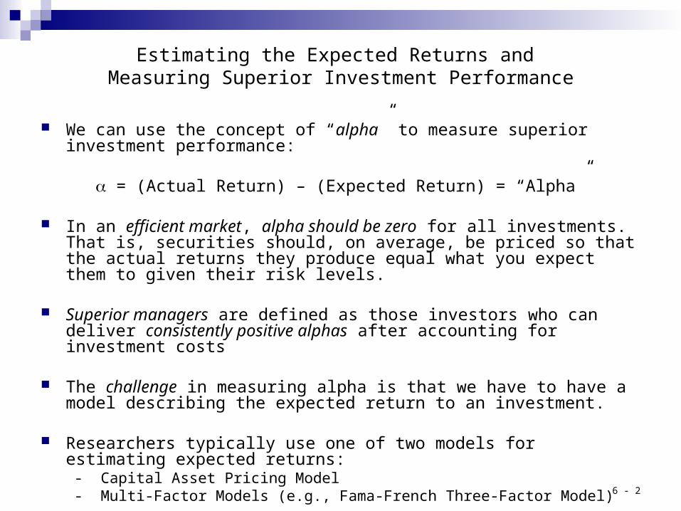
Estimating the Expected Returns and Measuring Superior Investment Performance

We can use the concept of “alpha” to measure superior investment performance:

= (Actual Return) – (Expected Return) = “Alpha”

In an efficient market, alpha should be zero for all investments. That is, securities should, on average, be priced so that the actual returns they produce equal what you expect them to given their risk levels.

Superior managers are defined as those investors who can deliver consistently positive alphas after accounting for investment costs

The challenge in measuring alpha is that we have to have a model describing the expected return to an investment.

Researchers typically use one of two models for estimating expected returns:

- Capital Asset Pricing Model - Multi-Factor Models (e.g., Fama-French Three-Factor Model)

6 - 3

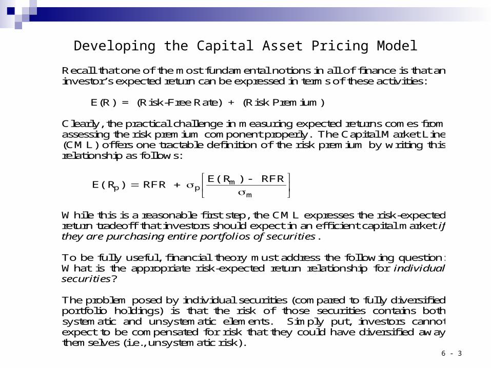
Developing the Capital Asset Pricing Model

Recall that one of the most fundamental notions in all of finance is that an investor’s expected return can be expressed in terms of these activities: E(R) = (Risk-Free Rate) + (Risk Premium) Clearly, the practical challenge in measuring expected returns comes from assessing the risk premium component properly. The Capital Market Line (CML) offers one tractable definition of the risk premium by writing this relationship as follows:

m

mpp

RFR )E(R RFR )E(R

While this is a reasonable first step, the CML expresses the risk-expected return tradeoff that investors should expect in an efficient capital market if they are purchasing entire portfolios of securities. To be fully useful, financial theory must address the following question: What is the appropriate risk-expected return relationship for individual securities? The problem posed by individual securities (compared to fully diversified portfolio holdings) is that the risk of those securities contains both systematic and unsystematic elements. Simply put, investors cannot expect to be compensated for risk that they could have diversified away themselves (i.e., unsystematic risk).

6 - 4

Developing the Capital Asset Pricing Model (cont.)

One way to handle this problem in the context of the CML is to adjust the number of “total risk” units that the investor assumes for security i (i.e., i) to account for just the systematic portion of that risk. This can be done by multiplying i by the security’s correlation with the market portfolio (i.e., rim):

m

mimii

RFR )E(R)r( RFR )E(R

Rearranging this expression leaves:

RFR] )[E(R r

RFR )E(R mm

imii

or: RFR] )[E(R RFR )E(R mii This is the celebrated Capital Asset Pricing Model (CAPM). Notice that the CAPM redefines risk in terms of a security’s “beta” (i.e., i), which captures that stock’s riskiness relative to the market as a whole. The graphical representation of the CAPM is called the Security Market Line (SML).

6 - 5

Using the SML in Performance Measurement: An Example

Two investment advisors are comparing performance. Over the last year, one averaged a 19 percent rate of return and the other a 16 percent rate of return. However, the beta of the first investor was 1.5, whereas that of the second was 1.0.

a. Can you tell which investor was a better predictor of individual stocks (aside from the issue of general movements in the market)?

b. If the T-bill rate were 6 percent and the market return during the period were 14 percent, which investor should be viewed as the superior stock selector?

c. If the T-bill rate had been 3 percent and the market return were 15 percent, would this change your conclusion about the investors?

6 - 6

Using the SML in Performance Measurement (cont.)

a. To tell which investor was a better predictor of individual stocks we look at their alphas. Alpha is the difference between their actual return an that predicted by the SML, given the risk of their individual portfolios. Without information about the parameters of this equation (risk-free rate and the market rate of return) we cannot tell which one is more accurate.

b. If RF = 0.06 and Rm = 0.14, then

Alpha1 = .19 – [.06+1.5(.14-.06)] = .19 - .18 = 0.01 Alpha2 = .16 – [.06+1(.14-.06)] = .16 - .14 = 0.02

Here, the second investor has the larger alpha and thus appears to be a more accurate predictor. By making better predictions the second investor appears to have tilted his portfolio toward undervalued stocks. c. If RF = 0.03 and Rm = 0.15, then

Alpha1 = .19 – [.03+1.5(.15 -.03)] = .19 - .21 = -0.02 Alpha2 = .16 – [.03+1(.15 -.03)] = .16 - .15 = 0.01

6 - 7

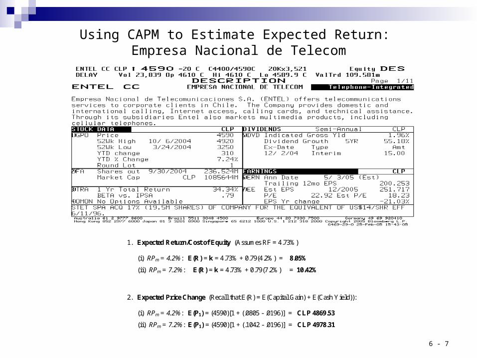
Using CAPM to Estimate Expected Return: Empresa Nacional de Telecom

1. Expected Return/Cost of Equity (Assumes RF = 4.73%)

(i) RPm = 4.2%: E(R) = k = 4.73% + 0.79(4.2%) = 8.05%

(ii) RPm = 7.2%: E(R) = k = 4.73% + 0.79(7.2%) = 10.42%

2. Expected Price Change (Recall that E(R) = E(Capital Gain) + E(Cash Yield)):

(i) RPm = 4.2%: E(P1) = (4590)[1 + (.0805 - .0196)] = CLP 4869.53

(ii) RPm = 7.2%: E(P1) = (4590)[1 + (.1042 - .0196)] = CLP 4978.31

6 - 8

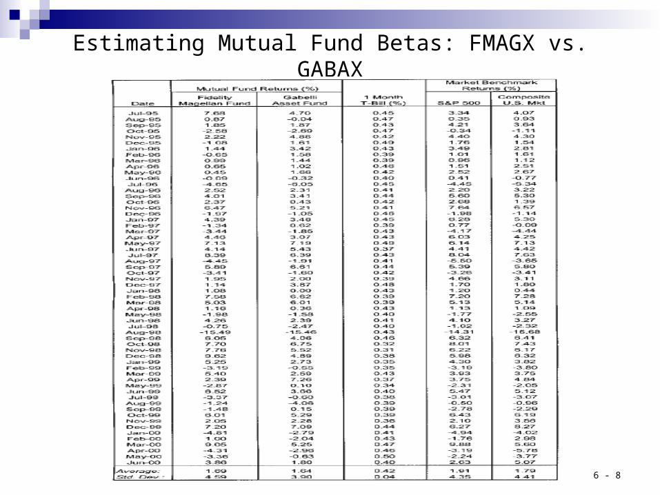
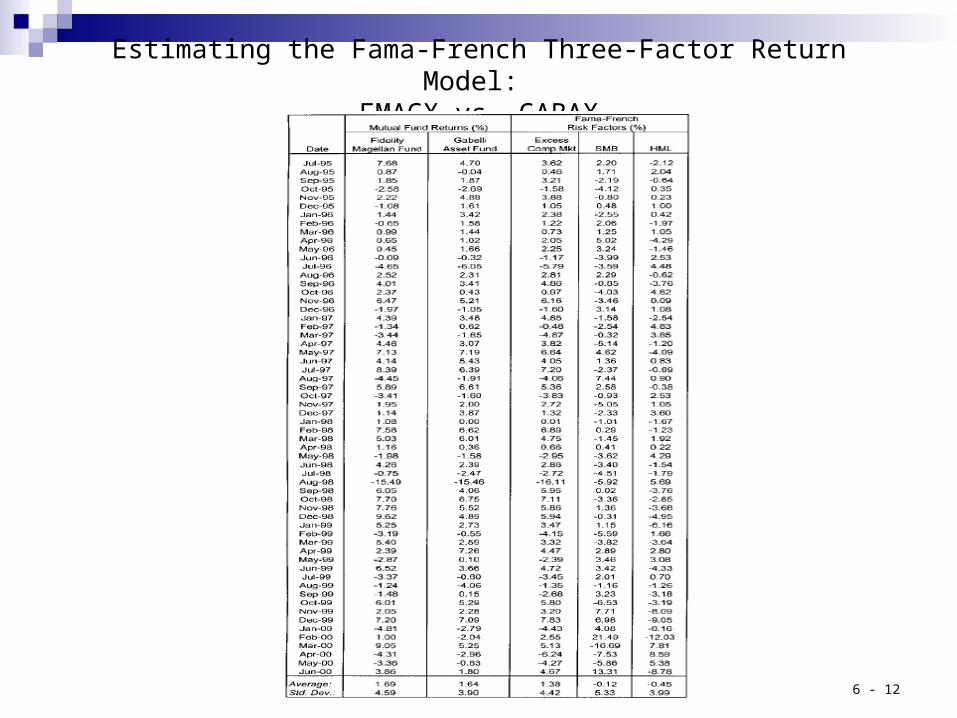
Estimating Mutual Fund Betas: FMAGX vs. GABAX

6 - 9

Estimating Mutual Fund Betas: FMAGX vs. GABAX (cont.)

6 - 10

Estimating Mutual Fund Betas: FMAGX vs. GABAX (cont.)

6 - 11

The Fama-French Three-Factor Model

The most popular multi-factor model currently used in practice was suggested by economists Eugene Fama and Ken French. Their model starts with the single market portfolio-based risk factor of the CAPM and supplements it with two additional risk influences known to affect security prices:

- A firm size factor- A book-to-market factor

Specifically, the Fama-French three-factor model for estimating expected excess returns takes the following form:

(Rit – RFRt) = i + bi1(Rmt – RFRt) + bi2SMBt + bi3HMLt + eit where, in addition to the excess return on a stock market portfolio, two other risk factors are defined: SMB (i.e., “Small Minus Big”) is the return to a portfolio of small capitalization stocks less

the return to a portfolio of large capitalization stocks HML (i.e., “High Minus Low”) is the return to a portfolio of stocks with high ratios of

book-to-market values (i.e., “value” stocks) less the return to a portfolio of low book-to-market value (i.e., “growth”) stocks

6 - 12

Estimating the Fama-French Three-Factor Return Model: FMAGX vs. GABAX

6 - 13

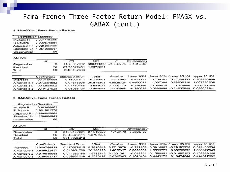
Fama-French Three-Factor Return Model: FMAGX vs. GABAX (cont.)

6 - 14

Fama-French Three-Factor Return Model: FMAGX vs. GABAX (cont.)

6 - 15

Style Classification Implied by the Factor Model

FMAGX *

* GABAX

Small

Large

Value Growth

6 - 16

Fund Style Classification by Morningstar

FMAGX GABAX

6 - 17

Active vs. Passive Equity Portfolio Management

The “conventional wisdom” held by many investment analysts is that there is no benefit to active portfolio management because:- The average active manager does not produce returns that exceed those

of the benchmark- Active managers have trouble outperforming their peers on a consistent

basis

However, others feel that this is the wrong way to look at the Active vs. Passive management debate. Instead, investors should focus on ways to:- Identifying those active managers who are most likely to produce

superior risk-adjusted return performance over time

This discussion is based on research authored jointly with Van Harlow of Fidelity Investments titled:

“The Right Answer to the Wrong Question: Identifying Superior Active Portfolio Management”

6 - 18

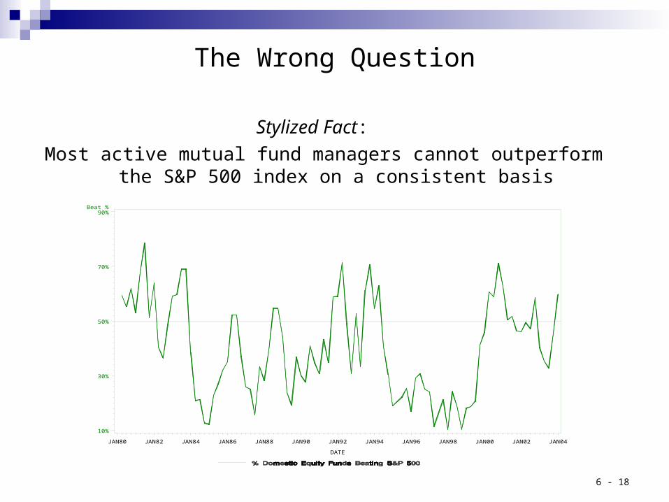
The Wrong Question

Stylized Fact:

Most active mutual fund managers cannot outperform the S&P 500 index on a consistent basis

Beat %

10%

30%

50%

70%

90%

DATE

JAN80 JAN82 JAN84 JAN86 JAN88 JAN90 JAN92 JAN94 JAN96 JAN98 JAN00 JAN02 JAN04

6 - 19

Beat %

10%

30%

50%

70%

90%

DATE

JAN80 JAN85 JAN90 JAN95 JAN00 JAN05

Small-Large

( 40%)

( 20%)

0%

20%

40%

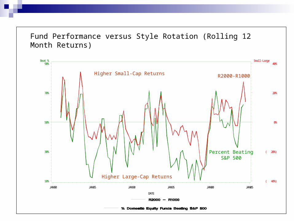
Higher Small-Cap Returns

Higher Large-Cap Returns

R2000-R1000

Percent BeatingS&P 500

Fund Performance versus Style Rotation (Rolling 12 Month Returns)

6 - 20

0102030405060708090

100

0 10 20 30 40 50 60 70 80 90100

S&P 500

Diversified Equity Mutual Funds

Stylized Fact: Most active mutual fund managers compete against

the “wrong” benchmark

The Wrong Question (cont.)

6 - 21

Defining Superior Investment Performance

Over time, the “value added” by a portfolio manager can be measured by the difference between the portfolio’s actual return and the return that the portfolio was expected to produce.

This difference is usually referred to as the portfolio’s alpha.

Alpha = (Actual Return) – (Expected Return)

6 - 22

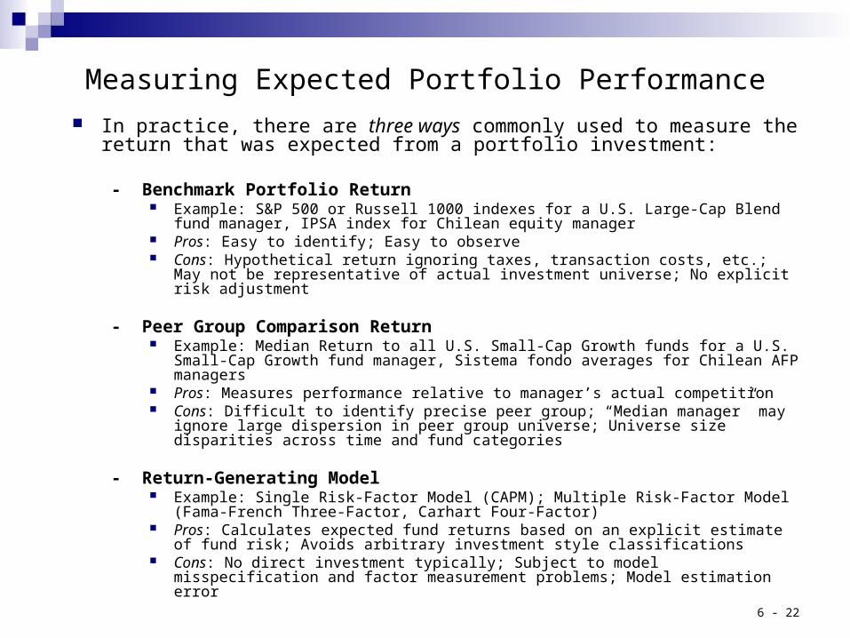
Measuring Expected Portfolio Performance

In practice, there are three ways commonly used to measure the return that was expected from a portfolio investment:

- Benchmark Portfolio Return Example: S&P 500 or Russell 1000 indexes for a U.S. Large-Cap Blend fund

manager, IPSA index for Chilean equity manager Pros: Easy to identify; Easy to observe Cons: Hypothetical return ignoring taxes, transaction costs, etc.; May not be

representative of actual investment universe; No explicit risk adjustment

- Peer Group Comparison Return Example: Median Return to all U.S. Small-Cap Growth funds for a U.S. Small-Cap

Growth fund manager, Sistema fondo averages for Chilean AFP managers Pros: Measures performance relative to manager’s actual competition Cons: Difficult to identify precise peer group; “Median manager” may ignore large

dispersion in peer group universe; Universe size disparities across time and fund categories

- Return-Generating Model Example: Single Risk-Factor Model (CAPM); Multiple Risk-Factor Model (Fama-

French Three-Factor, Carhart Four-Factor) Pros: Calculates expected fund returns based on an explicit estimate of fund risk;

Avoids arbitrary investment style classifications Cons: No direct investment typically; Subject to model misspecification and factor

measurement problems; Model estimation error

6 - 23

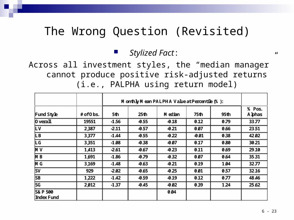
The Wrong Question (Revisited)

Stylized Fact:

Across all investment styles, the “median manager” cannot produce positive risk-adjusted returns (i.e., PALPHA using return model)

Monthly Mean PALPHA Value at Percentile (%):

Fund Style

# of Obs.

5th

25th

Median

75th

95th

% Pos. Alphas

Overall 19551 -1.56 -0.55 -0.18 0.12 0.79 33.77

LV 2,387 -2.11 -0.57 -0.21 0.07 0.66 23.51

LB 3,377 -1.44 -0.55 -0.22 -0.01 0.38 42.02

LG 3,351 -1.08 -0.38 -0.07 0.17 0.80 30.21

MV 1,413 -2.61 -0.67 -0.23 0.11 0.69 29.10

MB 1,691 -1.86 -0.79 -0.32 0.07 0.64 35.31

MG 3,169 -1.48 -0.63 -0.21 0.19 1.04 32.77

SV 929 -2.02 -0.65 -0.25 0.01 0.57 32.16

SB 1,222 -1.42 -0.59 -0.19 0.12 0.77 48.46

SG 2,012 -1.37 -0.45 -0.02 0.39 1.24 25.62

S&P 500 Index Fund

0.04

6 - 24

The Right Answer

When judging the quality of active fund managers, the important question is not whether: The average fund manager beats the benchmark The median manager in a given peer group produces a positive alpha

The proper question to ask is whether you can select in advance those managers who can consistently add value on a risk-adjusted basis Does superior investment performance persist from one period to the

next and, if so, how can we identify superior managers?

6 - 25

Lessons from Prior Research

Fund performance appears to persist over time

Original View: Managers with superior performance in one period are equally likely to produce superior or inferior performance in

the next period

Current View: Some evidence does support the notion that investment performance persists from one period to the next

The evidence is particularly strong that it is poor performance that tends to persist (i.e., “icy” hands vs. “hot” hands)

Security characteristics, return momentum, and fund style appear to influence fund performance

Security Characteristics: After controlling for risk, portfolios containing stocks with different market capitalizations, price-earnings ratios, and

price-book ratios produce different returns

Funds with lower portfolio turnover and expense ratios produce superior returns

Return Momentum: Funds following return momentum strategies generate short-term performance persistence

When used as a separate risk factor, return momentum “explains” fund performance persistence

6 - 26

Lessons from Prior Research (cont.)

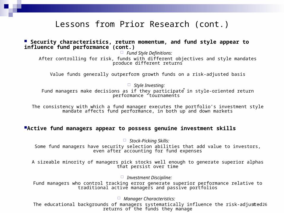
Security characteristics, return momentum, and fund style appear to influence fund performance (cont.)

Fund Style Definitions: After controlling for risk, funds with different objectives and style mandates produce different returns

Value funds generally outperform growth funds on a risk-adjusted basis

Style Investing: Fund managers make decisions as if they participate in style-oriented return performance “tournaments”

The consistency with which a fund manager executes the portfolio’s investment style mandate affects fund performance, in both up and down markets

Active fund managers appear to possess genuine investment skills

Stock-Picking Skills: Some fund managers have security selection abilities that add value to investors, even after accounting for fund

expenses

A sizeable minority of managers pick stocks well enough to generate superior alphas that persist over time

Investment Discipline: Fund managers who control tracking error generate superior performance relative to traditional active managers

and passive portfolios

Manager Characteristics: The educational backgrounds of managers systematically influence the risk-adjusted returns of the funds they

manage

6 - 27

CRSP (Center for Research in Security Prices) US Mutual Fund Database

Survivor-Bias Free database of monthly returns for mutual funds for the period 1962-2003

ScreensDiversified domestic equity funds only

Eliminate index funds

Require 30 prior months of returns to be included in the analysis on any given date

Assets greater than $1 million

Period 1979 – 2003 in order to analyze performance versus an index fund and have sufficient number of mutual funds

Return-generating model:Fama-French

E(Rp) = RF + {m[E(Rm) – RF] + sml[SML] + hml[HML]}

Style classification Map funds to Morningstar-type style categories based on Fama-French SML and HML

factor exposures (LV, LB, LG, MV, MB, MG, SV, SB, SG)

Data and Methodology for Performance Analysis

6 - 28

Methodology: Fund Mapped by Style Group

Mutual Fund Style Category:

Year LV LB LG MV MB MG SV SB SG Total

1979 9 23 70 0 3 21 0 3 27 156 1980 7 26 59 2 7 36 2 3 30 172 1981 5 20 32 1 6 39 0 3 25 131 1982 13 23 38 1 5 43 0 1 34 158 1983 14 27 60 1 7 31 0 2 42 184 1984 8 26 55 1 1 37 0 4 35 167 1985 7 23 74 3 1 37 7 1 30 183 1986 5 18 95 3 5 41 12 0 18 197 1987 6 22 80 3 2 51 14 5 16 199 1988 9 29 89 3 8 50 10 7 31 236 1989 12 30 92 2 3 54 0 11 43 247 1990 19 42 92 1 3 46 1 3 53 260 1991 25 63 97 3 3 44 0 2 48 285 1992 32 163 176 7 10 77 3 11 90 569 1993 38 202 166 8 5 92 2 19 103 635 1994 49 269 198 4 16 148 3 24 162 873 1995 57 210 224 20 67 234 24 97 264 1197 1996 86 405 421 20 45 279 47 83 262 1648 1997 160 535 478 52 111 357 83 106 324 2206 1998 355 636 601 160 130 256 133 172 356 2799 1999 469 456 827 157 107 641 261 119 412 3449 2000 771 604 992 316 82 587 215 142 459 4168 2001 812 680 1181 302 129 699 155 110 457 4525 2002 907 962 840 345 193 835 99 194 647 5022 2003 836 1250 1078 226 375 764 242 263 580 5614

6 - 29

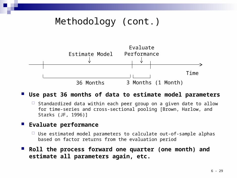
Use past 36 months of data to estimate model parameters Standardized data within each peer group on a given date to allow for time-

series and cross-sectional pooling [Brown, Harlow, and Starks (JF, 1996)]

Evaluate performance Use estimated model parameters to calculate out-of-sample alphas based on

factor returns from the evaluation period

Roll the process forward one quarter (one month) and estimate all parameters again, etc.

Estimate ModelEvaluate

Performance

36 Months 3 Months (1 Month)

Time

Methodology (cont.)

6 - 30

Distributions of Out-of-Sample Future Alphas (FALPHA)Quarterly – Equally Weighted 1979-2003

Performance Analysis

Quarterly FALPHA Value at Percentile (%):

Fund Style

# of Obs.

5th

25th

Median

75th

95th

% Pos. Alphas

Overall 126,613 -8.85 -3.12 -0.49 2.06 8.55 44.50

LV 17,195 -7.53 -2.98 -0.66 1.82 6.80 42.28

LB 23,566 -7.07 -2.43 -0.48 1.28 6.10 42.37

LG 30,642 -7.95 -2.66 -0.25 1.89 7.99 46.59

MV 6,214 -10.82 -3.13 -0.09 2.93 9.41 49.10

MB 4,251 -8.21 -3.23 -0.24 2.88 9.06 47.49

MG 19,172 -9.71 -3.79 -0.56 2.67 10.32 45.34

SV 4,963 -12.37 -4.39 -1.30 1.99 10.81 38.32

SB 4,475 -9.95 -3.96 -1.12 1.89 8.47 40.20

SG 16,135 -11.07 -4.03 -0.59 3.10 10.89 45.53

S&P 500 Index Fund

295 -1.41 -0.37 0.08 0.51 1.22 54.58

6 - 31

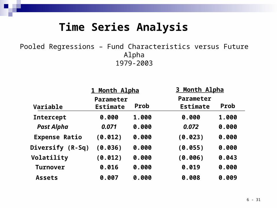
Pooled Regressions – Fund Characteristics versus Future Alpha1979-2003

Time Series Analysis

Parameter Variable

Parameter Estimate Prob Estimate Prob

Diversify (R-Sq)

Expense Ratio

Turnover

Assets

Intercept

Past Alpha

1 Month Alpha

3 Month Alpha

(0.036)

0.016

(0.012)

0.007

0.000

0.071

0.000

0.000

0.000

0.000

1.000

0.000

0.000

0.000

0.000

0.009

1.000

0.000

(0.055)

0.019

(0.023)

0.008

0.000

0.072

Volatility (0.012) 0.000 0.043(0.006)

6 - 32

Use past 36 months of data to estimate model parameters

Run a sequence of Fama-MacBeth cross-sectional regressions of future performance against fund characteristics and model parameters (alpha and R2 )

Average the coefficient estimates from regressions across the entire sample period

T-statistics based on the time-series means of the coefficients

Cross-Sectional Analysis

6 - 33

Cross-Sectional Performance Results

Parameter Variable

Parameter Estimate Prob Estimate Prob

Diversify (R-Sq)

Expense Ratio

Turnover

Assets

Past Alpha

1 Month Alpha

3 Month Alpha

(0.021)

0.015

(0.012)

0.008

0.047

0.091

0.034

0.033

0.034

0.000

0.333

0.072

0.063

0.190

0.000

(0.023)

0.022

(0.019)

0.009

0.061

Volatility (0.011) 0.377 0.306(0.022)

Fama-MacBeth Regressions – Fund Characteristics versus Future Alpha1979-2003

6 - 34

Logit Performance Analysis

Fund Characteristics versus a Positive Future Alpha1979-2003

Parameter Variable

Parameter Estimate Prob Estimate Prob

Diversify (R-Sq)

Expense Ratio

Turnover

Assets

Intercept

Past Alpha

1 Month Alpha

3 Month Alpha

(0.085)

0.028

(0.021)

0.015

(0.159)

0.082

0.000

0.000

0.000

0.000

0.000

0.000

0.000

0.000

0.000

0.000

0.000

0.000

(0.117)

0.022

(0.033)

0.023

(0.228)

0.093

Volatility (0.003) 0.419 0.000(0.022)

6 - 35

Probability of Finding a Superior Active Manager

Probability of Future Positive 3-month Alpha

Median Manager Controls for Turnover, Assets, Diversify, and Volatility

EXPR:

Std. Dev.

Group -2 (Low) -1 0 +1 +2 (High) (High –

Low)

-2 (Low)

0.4143

0.4062

0.3982

0.3903

0.3824

(0.0319)

-1

0.4369

0.4288

0.4206

0.4125

0.4045

(0.0324)

0

0.4599

0.4516

0.4434

0.4352

0.4270

(0.0329)

+1

0.4830

0.4746

0.4664

0.4581

0.4498

(0.0331)

+2 (High)

0.5061

0.4978

0.4895

0.4812

0.4729

(0.0333)

PALPHA:

(High – Low)

0.0918

0.0916

0.0913

0.0909

0.0905

6 - 36

Probability of Finding a Superior Active Manager (cont.)

Probability of Future Positive 3-month Alpha

“Best” Manager Controls for Turnover, Assets, Diversify, and Volatility

EXPR:

Std. Dev. Group

-2 (Low) -1 0 +1 +2 (High) (High – Low)

PALPHA: -2 (Low) 0.5051 0.4968 0.4884 0.4801 0.4718 (0.0333)

-1 0.5282 0.5199 0.5116 0.5033 0.4950 (0.0333)

0 0.5512 0.5430 0.5347 0.5264 0.5181 (0.0331)

+1 0.5741 0.5659 0.5577 0.5495 0.5412 (0.0328)

+2 (High) 0.5965 0.5885 0.5804 0.5723 0.5641 (0.0324)

(High – Low) 0.0915 0.0918 0.0920 0.0922 0.0923

6 - 37

Portfolio Strategies Based on Active Manager Search

-2.50%

-2.00%

-1.50%

-1.00%

-0.50%

0.00%

0.50%

1.00%

1.50%

2.00%

1 2 3 4 5 6 7 8 9 10

Ave

rag

e A

nn

ual

ized

Alp

ha

Asset Weighted Alpha Deciles - Quarterly Rebalance1979-2003

6 - 38

Asset Weighted - Quarterly RebalanceFormation Variables Separated by Upper and Lower Quartile Values

1979-2003

Portfolio Strategies (cont.)

Expense AlphaCumulative Value

of $1 InvestedAverage Alpha

(%)Alpha Volatility

(%)

Return Differential

(bp)

1.046 0.181 2.153

Lo 1.009 0.037 2.142 2Hi 1.005 0.018 4.025

Hi 1.515 1.691 3.371 291Lo 0.738 (1.221) 3.469

Lo Hi 1.446 1.502 3.596 309Hi Lo 0.673 (1.585) 4.712

1.022 0.088 1.700

Portfolio Formation Variables

Overall Sample

S&P 500 Index Fund

6 - 39

The Benefit of Selecting Good Managers and Avoiding Bad Managers

Positive Above Median Bottom TopAlpha Peer Peer Quartile Peer Quartile

No Information 44.3% 50.0% 24.4% 24.6%

Alpha 49.0% 54.2% 27.4% 27.7%Expense Ratio 46.0% 52.8% 27.1% 24.8%Alpha, Expense Ratio 50.6% 58.8% 28.8% 28.3%Alpha, Expense Ratio, Risk, Turnover, Assets 60.0% 62.9% 34.2% 48.7%

Overall Incremental Probability 15.7% 12.9% 9.8% 24.2%

Probability

6 - 40

Use past 9 months of daily data to estimate model and in-sample alpha

Optimize portfolio based on an assumption of risk aversion, i.e., risk-return tradeoff preference

Compute the performance of the portfolio over the next three (one) months

Roll the process forward each quarter and estimate all parameters again, etc.

Implementing a “Fund of Funds” Strategy: An Example

Estimate ModelEvaluate

Performance

9 Months 3 Months (1 Month)

Time

Methodology

6 - 41

EQPGX

EQPIXFAGCX

FAIVX

FALIX

FASOX

FATIX

FBTIX

FCLIX

FCNIX

FDCIX

FDGIX

FFSIX

FFYIX

FGIOX FHCIX

FHEIX

FMCCXFRVIX

FSCIX

FTIMX

FTQIX

FUGIX

FVIFXFVLIX

IVV

Cap

: Sm

all t

o La

rge

0

10

20

30

40

50

60

70

80

90

100

Value to Growth0 10 20 30 40 50 60 70 80 90 100

“Fund of Funds” Strategy

Fidelity Advisor Diversified Equity Fund Styles (6/04)

6 - 42

“Fund of Funds” Portfolio Strategy

Portfolio Weights Over Time

Name 200103 200106 200109 200112 200203 200206 200209 200212 200303 200306 200309 200312 200403Fidelity Advisor Equity Growth Instl 7.1% 5.3% 9.9% 9.6%Fidelity Advisor Equity Income Instl 20.0% 20.0% 20.0% 19.5% 20.0% 20.0% 12.0% 9.0% 5.3% 20.0%Fidelity Advisor Growth Opport Instl 13.4% 10.0% 2.6% 2.6% 10.8% 10.6% 14.5% 14.6% 6.1% 2.9%Fidelity Advisor Equity Value I 18.2% 18.6% 18.5% 18.8% 18.5% 10.4% 10.6% 10.6%Fidelity Advisor Large Cap Instl 7.0% 7.0%Fidelity Advisor Value Strat Instl 0.3% 4.5% 4.6% 4.9%Fidelity Advisor Technology Instl 8.0% 8.1% 7.5% 6.1% 5.6% 4.8% 4.2% 6.2% 5.0% 6.0% 7.3% 7.3% 5.6%Fidelity Advisor Cyclical Indst Instl 6.0% 7.4% 0.7% 4.9% 3.9% 4.1% 0.7% 1.2% 1.2% 10.9% 11.1%Fidelity Advisor Consumer Indst Instl 2.5% 1.4% 1.5% 2.5% 1.7%Fidelity Advisor Dynamic Cap App Inst 6.1% 9.3% 0.5%Fidelity Advisor Dividend Growth Inst 20.0% 20.0% 20.0% 20.0% 20.0% 2.1% 2.1% 7.6% 15.8% 15.9% 4.3% 4.2% 4.2%Fidelity Advisor Financial Svc Instl 9.3% 8.6% 7.8% 7.1% 1.2% 1.8% 11.8% 11.7% 11.5% 4.7% 12.3% 12.4% 15.1%Fidelity Advisor Growth & Income Inst 12.1% 16.7% 20.0% 17.1% 15.6% 7.4% 7.3% 11.1% 17.5% 17.4% 5.8% 5.7%Fidelity Advisor Health Care Instl 3.2% 2.2% 4.7% 4.5% 4.0% 8.8% 10.8% 9.7% 6.0% 5.7% 5.5% 5.5%Fidelity Advisor Mid Cap Instl 2.3% 9.6% 10.1% 8.6%Fidelity Advisor Telecomm&Util Gr Ins 0.9% 0.9% 5.0% 1.9% 5.0% 4.7% 4.7% 1.4%iShares S&P 500 Index 11.7% 15.2% 20.0% 7.8% 8.2% 8.1% 12.8% 14.9% 8.6% 8.5% 8.5% 12.3% 15.0%

Portfolio Characteristics

Portfolio

Avg Annual Active Return Periods

% Beat Bench in

Up Market

% Beat Bench in

Down MarketBest Active

Return

Worst Active Return

Longest Winning Streak

Longest Losing Streak

Annual Tracking

Error

S&P 500 0.68% 84 60% 67% 5.20% (3.7%) 7 4 3.3%

6 - 43

-0.1

0.0

0.1

0.2

0.3

0.4

0.5

0.6

0.7

0.8

JAN97 JAN98 JAN99 JAN00 JAN01 JAN02 JAN03 JAN04 JAN05

Cumulative Returns versus S&P 500

6 - 44

Active vs. Passive Management: Conclusions

Both passive and active management can play a role in an investor’s portfolio

Strong evidence for both positive and negative performance persistence (i.e., alpha persistence) Prior alpha is the most significant variable for forecasting future alpha

Expense ratio, risk measures, turnover and assets are also useful in forecasting future alpha

The existence of performance persistence provides a reasonable opportunity to construct portfolios that add value on a risk-adjusted basis