5L-25 - McGill Universitydigitool.library.mcgill.ca/thesisfile97944.pdf · ELECTRON ARC THERAPY...

ELECTRON ARC THERAPY USING AN ELEKTA

5L-25 LINEAR ACCELERATOR AT

MAISONNEUVE-ROSEMONT HOSPITAL

(MONTREAL, CANADA)

Caroline Duchesne

Medical Physics Unit

McGili University, Montréal

April 2006

A thesis submitted to McGiII University

in partial fulfillment of the

requirements for the degree of

Master of Science

in

Medical Physics

© Caroline Duchesne 2006

1+1 Library and Archives Canada

Bibliothèque et Archives Canada

Published Heritage Branch

Direction du Patrimoine de l'édition

395 Wellington Street Ottawa ON K1A ON4 Canada

395, rue Wellington Ottawa ON K1A ON4 Canada

NOTICE: The author has granted a nonexclusive license allowing Library and Archives Canada to reproduce, publish, archive, preserve, conserve, communicate to the public by telecommunication or on the Internet, loan, distribute and sell theses worldwide, for commercial or noncommercial purposes, in microform, paper, electronic and/or any other formats.

The author retains copyright ownership and moral rights in this thesis. Neither the thesis nor substantial extracts from it may be printed or otherwise reproduced without the author's permission.

ln compliance with the Canadian Privacy Act some supporting forms may have been removed from this thesis.

While these forms may be included in the document page cou nt, their removal does not represent any loss of content from the thesis.

• •• Canada

AVIS:

Your file Votre référence ISBN: 978-0-494-24659-7 Our file Notre référence ISBN: 978-0-494-24659-7

L'auteur a accordé une licence non exclusive permettant à la Bibliothèque et Archives Canada de reproduire, publier, archiver, sauvegarder, conserver, transmettre au public par télécommunication ou par l'Internet, prêter, distribuer et vendre des thèses partout dans le monde, à des fins commerciales ou autres, sur support microforme, papier, électronique et/ou autres formats.

L'auteur conserve la propriété du droit d'auteur et des droits moraux qui protège cette thèse. Ni la thèse ni des extraits substantiels de celle-ci ne doivent être imprimés ou autrement reproduits sans son autorisation.

Conformément à la loi canadienne sur la protection de la vie privée, quelques formulaires secondaires ont été enlevés de cette thèse.

Bien que ces formulaires aient inclus dans la pagination, il n'y aura aucun contenu manquant.

ACKNOWLEDGEMENTS

1 would like to extend my most heartfelt thanks to the many people that have helped me

bring this project to fruition. Most of ail, 1 would like to thank my supervisors, Maryse

Mondat and Wieslaw Wierzbicki. Their knowledge, experience and helpful advice were

invaluable to me in the completion of this work. Furthermore, their support and patience

permitted me to remain confident in my abilities regardless of the obstacles 1 faced

during the course of this project.

Much gratitude is also due to the "service de radiophysique" at Maisonneuve-Rosemont.

First and foremost, 1 would like to thank my colleagues, the physicists, Brigitte, Deborah,

Patrice, Richard, Noël and Étienne, who ail lent a hand at various points during this

work, whether it be providing technical support or providing agreeable companionship

during coffee breaks. 1 very much appreciate the warm welcome extended to me by the

group. 1 am also indebted to Simon Goulet (electronics) and Jean-René Tremblay

(machinist), whose talents and efficiency were essential to the success of this study.

Also, 1 would like to thank the technologists of Room 3 and the Mould Room for their

collaboration.

This project was made possible with support provided by the Health Minister of Quebec,

who 1 thank for this opportunity.

1 also extend thanks to the physicists at the Montreal General Hospital, particularly

Marina Olivares, who was kind enough to give me such valuable advice pertaining to my

subject. Thanks to my fellow students at McGili University with whom it was so pleasant

to share the past two years. Thanks also to Stanislas and Charles, my office mates.

Thanks to my parents who have always believed in me and who have done their utmost

to allow me to reach goals which initially appeared out of my reach. Finally, 1 would like

to thank Vincent who was always sure of my ability to complete a project of this

magnitude.

ii

ABSTRACT

Electron arc therapy is a special radiotherapeutic technique using a rotational electron

beam in the treatment of large superficial tumours following curved surfaces. In those

cases, arc therapy offers the best way to optimize dose uniformity while sparing healthy

tissues and critical organs. The use of this technique overcomes under or over dosage

problems caused by field junctions. However, electron arc therapy presents important

challenges in terms of dosimetry and treatment planning.

Clinical implementation of electron arc therapy requires the study of many parameters of

influence such as the radius of curvature of the treated surface, the width of the

treatment field, the total angle of irradiation and the beam energy. Monitor unit

calculation to deliver prescribed dose is a very critical topic and, in general, requires

acquisition of a large amount of measured dosimetric data.

This project concerns the clinical implementation of electron arc therapy using an Elekta

SL-25 linear accelerator in the radiation oncology department of the Maisonneuve

Rosemont Hospital (Montreal, Canada). Firstly, the objective of the study is to observe

the influence of the radius of curvature, the total arc angle and the field width on the

following dosimetric parameters: depth of maximum dose, isodose distributions and

electron arc beam output at the depth of maximum dose. Secondly, for our particular

setup, the goal is to develop a simple monitor unit calculation method, based on an

analytical model fitted through measured dosimetric data covering a large range of

possible clinical situations.

ln order to achieve these goals, electron arc irradiations were performed on cylindrical

acrylic phantoms of different radii, successively varying the total arc angle and the field

width at isocentre. Results obtained with thermoluminescent dosimeters show a minor

impact of the radius of curvature variation on the percent depth dose curves. However,

they show a significant impact on the beam output. It was also observed that the total

arc angle influences the dose at the depth of maximum dose only up to a limit angle

value, different for each radius of curvature. Finally, the field width at isocentre has an

impact on the beam output as weil as on the bremsstrahlung contribution at the

isocentre.

iii

Concerning the monitor unit calculation, a seven parameter analytical model fitted

through measured data was obtained using Origin 7 software. A relationship giving the

beam output as a function of the radius of curvature and the total arc angle was found.

The field width was not included in the model, but will be part of further investigation

before clinical implementation. As future work, dosimetric measurements with other

energies should be carried on, mainly to be able to cover a wider range of clinical cases.

iv

RÉSUMÉ

La thérapie en arc par faisceau d'électrons est une technique spéciale de radiothérapie

utilisant un faisceau d'électrons en rotation lors du traitement de tumeurs superficielles

suivant des surfaces courbes de grande étendue. Pour ce type de tumeurs, la thérapie

en arc constitue la meilleure façon d'optimiser l'homogénéité de la dose tout en

épargnant les tissus sains et les organes à risque. De plus, les problèmes de sur

dosage ou de sous-dosage causés par des jonctions de champs sont éliminés.

Cependant, cette technique présente des défis considérables, tant au niveau technique

qu'au niveau de la dosimétrie et de la planification de traitement.

L'implantation clinique de la thérapie en arc par faisceau d'électrons nécessite l'étude de

plusieurs paramètres d'influence tels le rayon ae courbure de la surface à traiter, la

largeur du champ de traitement, la grandeur de l'arc total d'irradiation et l'énergie du

faisceau d'électrons. Le calcul du nombre d'unités moniteur devient possible suite à

l'acquisition d'une grande série de mesures dosimétriques.

Ce projet porte sur l'implantation de la thérapie en arc par faisceau d'électrons utilisant

un accélérateur linéaire Elekta SL-25 au département de radio-oncologie de l'hôpital

Maisonneuve-Rosemont (Montréal, Canada). L'objectif de cette étude est tout d'abord

de mettre en lumière l'influence du rayon de courbure du patient, de l'angle total de l'arc

et de la largeur de champ sur les paramètres dosimétriques suivants: la profondeur de la

dose maximale, les courbes d'isodoses et le débit de dose à la profondeur de la dose

maximale. Ensuite, pour notre montage particulier, le but est de développer une

méthode simple de calcul du nombre d'unités moniteur basée sur un modèle analytique

ajusté aux données dosimétriques mesurées couvrant un large éventail de situations

cliniques possibles.

Pour ce faire, des irradiations en arc ont été pratiquées sur des mannequins cylindriques

en variant successivement le rayon de courbure, la grandeur d'arc et la largeur de

champ. Les résultats obtenus grâce aux dosimètres thermoluminescents montrent un

impact mineur de la variation du rayon de courbure sur les rendements en profondeur,

mais une influence majeure de ce paramètre sur le débit de dose. Quant à la grandeur

d'arc, son impact sur la dose maximale se fait sentir seulement jusqu'à une valeur

v

d'angle limite, différente pour chaque rayon de courbure. Finalement, une influence de la

largeur du champ à l'isocentre fut observée au niveau du débit de dose ainsi qu'au

niveau de la proportion de la radiation bremsstrahlung à l'isocentre.

En ce qui concerne le calcul d'unités moniteur, un modèle analytique comportant sept

paramètres et ajusté aux données dosimétriques mesurées fut obtenu grâce à

l'utilisation du logiciel Origin 7. Ce modèle met en relation le débit de dose à la

profondeur de dose maximale avec le rayon de courbure de la surface à traiter et l'angle

total d'irradiation. La largeur du champ à l'isocentre n'est pas incluse dans ce modèle et

fera l'objet d'une étude plus poussée avant l'implantation clinique. De plus, des mesures

impliquant d'autres énergies nominales du faisceau d'électrons devraient être

effectuées, principalement dans le but d'élargir l'utilisation de la technique à un plus

grand nombre de cas cliniques.

vi

TABLE OF CONTENTS

ACKNOWLEDGEMENTS ................................................................................................ ii

ABSTRACT .................................................................................................................... iii

RÉSUMÉ ......................................................................................................................... v

TABLE OF CONTENTS ................................................................................................. vii

LIST OF TABLES ........................................................................................................... xi

LIST OF FIGURES ........................................................................................................ xii

LIST OF SYMBOLS AND ACRONYMS ........................................................................ xvi

CHAPTER 1 - INTRODUCTION ..................................................................................... 1

1.1 General information ............................................................................................... 1

1.2 Project description ................................................................................................. 2

CHAPTER 2 - THEORETICAL BACKGROUND ............................................................. 3

2.1 Characteristics of clinical electron beams .............................................................. 3

2.1.1 Central axis depth dose distributions .............................................................. 5

2.1.1.1 Effect of energy ........................................................................................ 7

2.1.1.2 Effect of field size ..................................................................................... 8

2.1.1.3 Effect of oblique incidence ........................................................................ 9

2.1.2 Isodose distributions ..................................................................................... 11

2.1.3 Clinical electron beam delivery ..................................................................... 12

2.1.3.1 Linear accelerator .................................................................................. 12

2.1.3.2 Beam output ........................................................................................... 13

2.2 Electron arc therapy ............................................................................................ 13

2.2.1 Materials and methods .................................................................................. 14

2.2.1.1 Treatment machine ................................................................................ 14

2.2.1.2 Treatment setup ..................................................................................... 15

2.2.2 General behaviour of electron arc distributions ............................................. 17

2.2.2.1 Depth of isocentre .................................................................................. 17

2.2.2.2 Field size ................................................................................................ 18

2.2.2.3 T ertiary collimation ................................................................................. 19

2.2.2.4 Photon contamination ............................................................................. 20

2.2.3 Dosimetry and treatment planning ................................................................ 21

2.2.3.1 Integration method ................................................................................. 22

2.2.3.2 Direct measurement method .................................................................. 24

vii

2.3 Practical dosimetry in high-energy electron beams ............................................. 28

2.3.1 lonization chambers ...................................................................................... 28

2.3.1.1 Basic principle ........................................................................................ 28

2.3.1.2 Relative dosimetry .................................................................................. 29

2.3.1.3 Calibration of high-energy electron beams ............................................. 30

2.3.2 Radiographie films ........................................................................................ 31

2.3.2.1 Photographie emulsion principle ............................................................. 31

2.3.2.2 Dosimetry ............................................................................................... 32

2.3.2.3 Film position with respect to beam axis direction .................................... 33

2.3.3 Thermoluminescent dosimeters .................................................................... 34

2.3.3.1 Thermoluminescence principle ............................................................... 35

2.3.3.2 Dosimetry ............................................................................................... 36

2.3.3.3 Characteristics of LiF :Mg,Ti (TLD-100) .................................................. 37

CHAPTER 3 - MATERIALS AND METHODS ............................................................... 39

3.1 Materials ............................................................................................................. 39

3.1.1 Applicators and masks .................................................................................. 39

3.1.2 Phantoms ..................................................................................................... 39

3.1.3 Detectors ...................................................................................................... 42

3.2 Detector calibration ............................................................................................. 42

3.2.1 Depth scaling ................................................................................................ 42

3.2.2 NACP parallel-plate cham ber calibration ....................................................... 44

3.2.3 Film calibration ............................................................................................. 45

3.2.3.1 Calibration in solid water and acrylic ...................................................... 45

3.2.3.2 Energy dependence verification ............................................................. 45

3.2.4 TLD calibration ............................................................................................. 46

3.2.4.1 General TLD handling ............................................................................ 46

3.2.4.2 Individual TLD calibration ....................................................................... 47

3.2.4.3 Non linearity correction of the dose response ......................................... 47

3.2.4.4 Conversion of TL response to dose ........................................................ 48

3.2.4.5 Energy dependence verification ............................................................. 49

3.3 Static POO measurements .................................................................................. 49

3.3.1 ln water ......................................................................................................... 49

3.3.2 ln solid water ................................................................................................ 49

3.3.3 ln acrylic ....................................................................................................... 50

viii

3.4 Arc irradiations .................................................................................................... 50

3.4.1 Dosimetric measurements ............................................................................ 50

3.4.1.1 Electron arc setup .................................................................................. 50

3.4.1.2 Radial PDDs ........................................................................................... 51

3.4.1.3 20 dose distributions .............................................................................. 53

3.4.2 Predictive model for beam output ................................................................. 54

CHAPTER 4 - RESUL TS AND DiSCUSSiON ............................................................... 57

4.1 Detector calibration ............................................................................................. 57

4.1.1 Depth scaling ................................................................................................ 57

4.1.2 NACP ionization chamber .............................................................................. 59

4.1.3 Films ............................................................................................................. 59

4.1.3.1 Film calibration curve ............................................................................. 59

4.1.3.2 Film energy dependence verification ...................................................... 61

4.1.4 TLDs ............................................................................................................. 62

4.1.4.1 Individual TLD calibration ....................................................................... 62

4.1.4.2 Non linearity correction of the dose response ......................................... 63

4.1.4.3 Conversion of TL response to dose ........................................................ 64

4.1.4.4 TLD energy dependence verification ...................................................... 65

4.2 Static POO measurements: film and TLD reliability ............................................. 65

4.2.1 ln water and solid water ................................................................................ 65

4.2.2 ln acrylic ....................................................................................................... 66

4.3 Arc irradiations .................................................................................................... 67

4.3.1 Dosimetric measurements ............................................................................ 67

4.3.1.1 Radial PDDs ........................................................................................... 67

Effect of di .......................................................................................................... 70

Effect of a .......................................................................................................... 72

Photon contamination ........................................................................................ 75

Effect of w .......................................................................................................... 76

4.3.1.220 dose distributions .............................................................................. 77

4.3.2 Predictive model for beam output ................................................................. 82

4.3.2.1 Model elaboration ................................................................................... 82

4.3.2.2 Model validation ..................................................................................... 84

4.3.2.3 Field width effect .................................................................................... 85

4.3.2.4 Future work ............................................................................................ 86

ix

4.4 Clinical implementation ....................................................................................... 88

CHAPTER 5 - CONCLUSiON ....................................................................................... 91

REFERENCES ............................................................................................................. 94

x

LIST OF TABLES

Table 2.1 Expected uncertainty on relative dose measurements with films (Modified

from Dutreix and Dutreix 1969) .............................................................................. 33

Table 3.1 Applicators and masks used in the different parts of the study .................. 39

Table 3.2 Phantoms used in the different parts of the study ...................................... 40

Table 3.3 Detectors and related reading equipment. ................................................. 42

Table 3.4 Recommended values of Cp! for solid water and acrylic (From Thwaites et al

2003) ................................................................................................................... 43

Table 3.5 List of parameters for radiographic film energy dependence verification .... 46

Table 3.6 Irradiation conditions for obtention of TLD calibration curve ....................... 48

Table 3.7 List of parameters for TLD energy dependence verification ....................... 49

Table 3.8 Summary of ail experimental arc parameters used in film and TLD

measurements ....................................................................................................... 51

Table 3.9 Experimental setup for verification measurements .................................... 55

Table 4.1 Depth scaling parameters .......................................................................... 57

Table 4.2 Calibration coefficient for the NACP parallel-plate ionization chamber used in

daily output measurements .................................................................................... 59

Table 4.3 Values of depth of maximum dose in acrylic for each cylindrical phantom, for

~160° and w=7.3 cm ............................................................................................ 71

Table 4.4 Values of the bremsstrahlung contribution at the isocentre, PDDx, from

electron arc irradiations of Œ= 1200 with w = 7.3 cm .............................................. 75

Table 4.5 Values of fitting parameters in the analytical predictive model of the beam

output. .................................................................................................................. 83

Table 4.6 Calculated (predictive model) and measured beam output for electron arc

irradiation in a 12.7 cm radius phantom with w=7.3 cm .......................................... 85

Table 4.7 Therapeutic range in acrylic and in water as a function of di, taken from

radial PDD measurements in arc irradiations with ~160° and w=7.3 cm .............. 89

xi

LIST OF FIGURES

Figure 2.1 Rate of energy loss in MeV/g·cm2 as a function of electron energy for

water and lead (Adapted from Khan 2003) .............................................................. 3

Figure 2.2 Typical electron beam percentage depth dose curve (Adapted from

Strydom et a/2003) . ................................................................................................ 5

Figure 2.3 Central axis POO curves for a family of electron beams from a high

energy linear accelerator (From Strydom et a/2003) . .............................................. 7

Figure 2.4 Schematic illustration showing the increase in percent surface dose with

an increase in electron energy (Adapted from Khan 2003) ...................................... 8

Figure 2.5 POO curves for different field sizes for a 20 MeV electron beam from a

linear accelerator (From Strydom et a/2003) . .......................................................... 9

Figure 2.6 POO curves for various beam incidences for a 9 MeV (a) and 15 MeV (b)

electron beam (From Strydom et a/2003) .............................................................. 10

Figure 2.7 Schematic illustration of how the relative orientation of pencil beams

changes with the angle of obliquity (Adapted from Khan 2003) .............................. 10

Figure 2.8 Comparison of isodose curves for different energy electron beams

(Adapted from Khan 2003) .................................................................................... 11

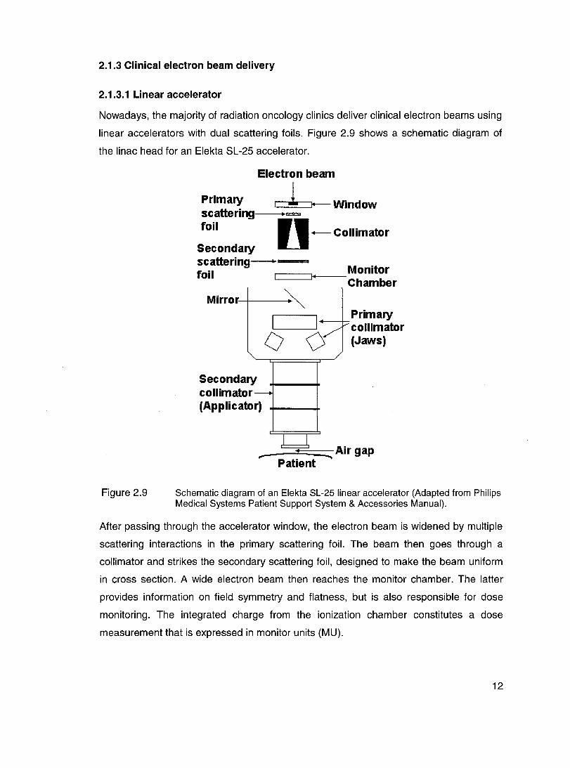
Figure 2.9 Schematic diagram of an Elekta SL-25 linear accelerator (Adapted from

Philips Medical Systems Patient Support System & Accessories Manual) ............. 12

Figure 2.10 Schematic diagram of the setup used in electron arc therapy ................ 16

Figure 2.11 Patient in treatment position shows cast outlining target volume (From

McNeely et a/1988) ............................................................................................... 17

Figure 2.12 Measured radial electron beam POOs for electron arc therapy with

various combinations of depth of isocentre di and field width w for constant w = 7 cm

(From Pla et a/1988) . ............................................................................................ 18

Figure 2.13 Measured radial electron beam POOs for electron arc therapy with

various combinations of depth of isocentre di and field width w for constant

di = 15 cm (From Pla et a/1988) . ........................................................................... 19

Figure 2.14 Isodose distribution in arc rotation with and without lead strips at the ends

of the arc, using a section of an Alderson Rando phantom closely simulating an

actual patient cross section (Adapted from Khan et a/1977) . ................................ 20

Figure 2.15 Measured percentage depth doses for rotational electron beams with an

electron energy of 15 MeV (From Pla et a/1989) ................................................... 20

xii

Figure 2.16 Geometry used in the calculation of the characteristic angle /3 (From Pla

et a/1988) . ............................................................................................................ 25

Figure 2.17 Measured radial PDD curves for electron arc therapy with (a) /3 = 40° and

(b) /3= 80° for a beam energy of 9 MeV (From Pla et a/1988) ............................... 26

Figure 2.18 Geometry and definition of parameters used in dose calculation for a

pseudoarc irradiation (Adapted from Pla et a/1988) . ............................................. 27

Figure 2.19 Schematic diagram of the circuitry for an ionization chamber-based

dosimetry system (From Andreo et a/2003) . ......................................................... 28

Figure 2.20 Film artefacts created by misalignment of the film in the phantom. The

effects of (a) air gaps between the film and the phantom, (b) film edge extending

beyond the phantom, and (c) film edge recessed within the phantom (Adapted from

Khan 2003) ............................................................................................................ 34

Figure 2.21 Schematic energy-Ievel diagram of an insulating crystal that exhibits TL

due to radiation (Adapted from Cameron et a/1968) . ............................................ 35

Figure 2.22 An example of glow curve of LiF (TLD-100) after phosphor has been

annealed at 400°C for 1 hour and read immediately after irradiation showing 5

peaks with their respective half-lite (Adapted from Khan 2003) .............................. 37

Figure 3.1 TLD plates for arc irradiations: (a) non-aligned configuration and (b)

vertically aligned configuration ............................................................................... 41

Figure 3.2 Calibration plate for TLDs ...................................................................... 41

Figure 3.3 Geometryof an electron arc therapy technique ..................................... 51

Figure 3.4 Combinations of experimental parameters used for TLD measurements in

electron arc irradiations ......................................................................................... 52

Figure 3.5 Schematic diagram of the irradiation setup for tertiary collimation

verification with films: (a) Film #1, (b) Film #2 ........................................................ 53

Figure 4.1 (a) Central axis percent depth ionization curves in acrylic and in solid

water; (b) Central axis depth dose curves .............................................................. 58

Figure 4.2 Sensitometrie curve for X-Omat-V films performed in a 10 MeV electron

beam in sol id water at depth of dose maximum dmax(sw)=2 cm with a 20x20 cm2 field

and SSD 100 cm ................................................................................................... 60

Figure 4.3 Comparison between sensitometrie curves of X-Omat-V films performed

at dmax in acrylic and in solid water for the same irradiation conditions: 10 MeV,

20x20 cm2, SSD 100 cm ........................................................................................ 61

xiii

Figure 4.4 Sensitometric curves of X-Omat-V films measured at different depths in a

sol id water phantom for a 10 MeV beam, 20x20 cm2 mask, SSD 100 cm .............. 62

Figure 4.5 Calibration curve for the whole TLD batch, performed at dmax . ............... 63

Figure 4.6 Calibrations at dmax and at d=4.2 cm ...................................................... 65

Figure 4.7 Static PDDs in water and solid water measured with different detectors

using 10 MeV nominal energy, arc applicator with a 6x20 cm2 mask and SSD

100 cm. .. ............................................................................................................ 66

Figure 4.8 Static PDD in a fiat acrylic phantom measured with TLDs and X-Omat-V

film using 10 MeV nominal energy, arc applicator with a 6x20 cm2 mask and SSD

100 cm .............................................................................................................. 67

Figure 4.9 Radial PDD measured with TLDs and X-Omat-V film in an electron arc

irradiation using 10 MeV nominal energy, arc applicator with a 6x20 cm2 mask and

SSD 100 cm .......................................................................................................... 68

Figure 4.10 Radial PDDs measured with TLDs in an electron arc irradiation with

di=10.2 cm, w=7.3 cm and a=160° for both TLD configurations ............................. 69

Figure 4.11 Radial PDDs measured with TLDs for a fixed w of 7.3 cm, a=160° and

varying di values .................................................................................................... 70

Figure 4.12 Radial depth dose distributions measured with TLDs for a fixed w of

7.3 cm, a=160°, varying di values and the same number of MUs ........................... 72

Figure 4.13 Radial PDDs measured with TLDs for a fixed w of 7.3 cm with di=10.2 cm

and varying avalues ............................................................................................. 73

Figure 4.14 Dose at dmax measured with TLDs for every di and avalue, for a field width

w=7.3 cm ............................................................................................................... 74

Figure 4.15 Schematic diagram explaining the effect of a on the dose at dmax for

different di values" ................................................................................................... 75

Figure 4.16 Radial PDDs measured with TLDs for a=160° and varying w values. (a)

di=5.1 cm; (b) di=7.6 cm; (c) di=10.2 cm; (d) di=15.2 cm ........................................ 77

Figure 4.17 Comparison of isodose distributions for an electron arc irradiation with

w=7.3 cm and a=160° (a) di=5.1 cm; (b) di=10.2 cm .............................................. 78

Figure 4.18 Comparison of isodose distributions for an electron arc irradiation with

d;=10.2 cm and w=7.3 cm (a) a=60o; (b) a=1200 .................................................... 80

Figure 4.19 Comparison of two different configurations for tertiary collimation (a) lead

strips on the left arc limit; (b) lead strips inside the left arc limit. ............................. 81

xiv

Figure 4.20 (a) Plot of the average beam output as a function of (1/d/). The fitting

curve is an asymptotic relationship (equation 3.10); (b) Histogram of errors on the

average output. ...................................................................................................... 82

Figure 4.21 Plots of fitting parameters of equation 3.10 as a function of the total arc

angle a (equations 3.11 to 3.13) (a) a vs a; (b) b vs a; (c) log1Qc vs a .................... 84

Figure 4.22 Beam output as a function of field width for electron arc irradiations with

varying di values .................................................................................................... 85

Figure 4.23 Dispersion of measured output data relatively to average values .......... 86

Figure 4.24 (a) Comparison between measured data (dots) and curves (solid lines)

generated by the predictive model; (b) Histogram of errors: fitted beam output

compared to measured beam output for ail individual measurements .................... 88

xv

LIST OF SYMBOLS AND ACRONYMS

AAPM

a.u.

CT

EDR

f

IMRT

IPEM

Linac

MU

OD

PDD

OA

PDI

Rso

American Association of Physicists in Medicine

Arbitrary units

Computerized Tomography

Isocentre depth

Depth of dose maximum

Extended Dose Range

Nominal source-to-axis distance

Intensity modulated radiation therapy

Institute of Physics and Engineering in Medicine

Linear accelerator

Monitor Unit

Optical density

Percent depth dose

Oualityassurance

Percent depth ionization

Practical range

Depth of 90% dose, therapeutic range

Depth of 50% dose

xvi

SAD

SSD

TL

(TLi )200

TLD

TPS

TTP

w

z

Beam quality index

Source-to-axis distance

Source-to-surface distance

Thermoluminescence reading

Average TL for 3 individual TLD calibration readings

Average of ail (TL;)200 of the TLD batch

Average TL of a group of 5 TLDs irradiated to a given number of

MUs

Average TL response of the whole TLD batch irradiated to a given

number of MUs

Average TL of a group of 5 TLDs from individual calibration at

200 MU

Thermoluminescent dosimeter

Treatment Planning System

Time-Temperature Profile

Field width at isocentre

Atomic number

xvii

CHAPTER 1 - INTRODUCTION

1.1 General information

ln radiation therapy, treatment of superficial tumours with electrons is usually performed

using stationary beams collimated by electron applicators or cones. However, this

technique presents problems of non uniformity of dose which can be unacceptable

clinically when tumours along large curved surfaces are involved. For example,

treatment in post-mastectomy breast cancer patients requires irradiation of the chest

wall and regional Iymphatics. Thorax curvature, the varying depths of the target volumes

and the proximity of underlying lung make this treatment technically challenging. For a

large chest, electron field abutment is necessary, resulting in over or under dosage at

the field junction. The use of tangential photon fields also becomes a problem in these

cases, leading to excessive irradiation of the lung. Electron arc irradiation then becomes

the method of choice in a variety of clinical situations involving superficial treatment of

large curved surfaces. This technique can be used with a curative intent for a variety of

cases such as post-mastectomy breast carcinoma, chest wall Iymphoma, scalp

angiosarcoma and scalp Iymphoma. It is also used in palliative treatment of locally

extensive breast carcinoma.


beam in the treatment of large superficial volumes along curved surfaces. For su ch


tissue and critical organs. Historically, Becker and Weitzel were the first to describe the

principle and practical application of this technique in 1956. The implementation of

electron arc therapy is characterized by several difficulties: the fairly lengthy time

required to plan each treatment, the unavailability of a suitable commercial treatment

planning system and the relatively small number of patients who require this kind of

treatment. In consequence, electron arc therapy is not used in many clinics in North

America. Moreover, its physical characteristics are poorly understood. The dose

distributions depend on several parameters such as electron energy, patient curvature,

field width and shape, as weil as tertiary collimation.

1

1.2 project description

The main goal of this study is the implementation of electron arc irradiation in the

radiation oncology department of Maisonneuve-Rosemont Hospital (Montreal, Canada).

ln order to realize this goal, the principal properties of electron arc treatments had to be

investigated.

Firstly, the influence of the radius of curvature, the total arc angle and the field width on

dosimetric parameters su ch as depth of maximum dose, isodose distributions and

electron arc beam output at the depth of maximum dose was studied. Electron arc

irradiations were performed on cylindrical acrylic phantoms of different radii (from 5.1 to

15.2 cm), successively varying the total arc angle (60 to 160°) and the field width at

isocentre (3.7 to 9.8 cm). Radial depth dose curves and beam output measurements

were performed with thermoluminescent dosimeters and isodose distributions were

obtained with X-Omat-V films. The contribution of the photon contamination to the dose

and the effect of tertiary collimation were investigated as weil.

Secondly, based on a bank of dosimetric data from TLD measurements in electron arc

irradiations, an analytical model for monitor unit calculation was developed. The fitted

data set covers a wide range of clinical situations. Additional measurements were

performed to verify the predictive ability of the analytical model, using different phantom

sizes and arc angles.

ln this work, a theoretical background on clinical electron beams, detectors of interest for

electron beam measurements and a review of what has been done concerning electron

arc therapy is first presented. Then, a detailed description of the materials and methods

used in this study is given. Ali results are then presented and discussed. Finally,

recommendations for future work and ameliorations of the technique necessary before

clinical implementation are suggested.

2

CHAPTER 2 - THEORETICAL BACKGROUND

2.1 Characteristics of clinical electron beams

Electrons traveling through a medium interact with atoms via four main processes

involving Coulomb force interactions: inelastic collisions with atomic electrons (Ieading to

ionization and excitation), inelastic collisions with nuclei (radiative interactions) and

elastic collisions with atomic electrons and with nuclei. In the process of collision with

atomic electrons, if the ejected electron acquires enough kinetic energy to produce

further ionization, the electron is called a secondary electron or c5-ray. An electron beam

is considered to be ionizing radiation because of these possible interactions with matter.

When an electron beam goes through a medium, the energy is degraded continually

until electrons reach thermal energies and are captured by surrounding atoms (Khan

2003, p. 297). For a therapy electron beam, the typical rate of energy loss in water is

approximatively 2 MeV/cm. The magnitude of collisional and radiative processes for

electrons traveling in water and lead are shown in Figure 2.1 .

Figure 2.1

10 r-~~--~-------'--------r-------'

Lead Collisional

1

i i

0.01 '--~~~'-'-'-~~~LLLL __ ~~~-'-----~~~"-,-,

0.01 0.1 10 100

Electron energy [MeV]

Rate of energy loss in MeV/g.cm2 as a function of electron energy for water and lead (Adapted from Khan 2003).

The mass stopping power of a medium, (S/p) , is defined as the rate of energy loss by a

charged particle per gram per centimeter squared, as shown in equation 2.1 :

1 dE

P dl (2.1 )

3

where p is the density of the absorbing medium and dE is the total energy lost by the

electron traversing a path length dl. The total mass stopping power can be expressed as

a contribution of both collisional, (S/p)cot. and radiative, (S/P)rad, losses:

(2.2)

Figure 2.1 shows that for collisional interactions, the rate of energy loss depends on the

incident electron energy and on the electron density of the medium. The mass collisional

stopping power is greater for low atomic number (Z) materials than for high Z materials.

This is because high Z materials have a lower electron density than low Z materials and

because they have more tightly bound electrons, which are less available for collisional

interactions. For example, collisional stopping power is higher in water than in lead

since, as a low Z material, the main source of energy losses is ionizing events.

For radiative interactions, also called bremsstrahlung production, the rate of energy loss

is proportional to the electron energy and to the square of the atomic number of the

absorbing material. Bremsstrahlung production is then more efficient for high-energy

electrons and for high Z materials, such as lead (see Figure 2.1).

However, in the determination of the energy absorbed per unit mass in a medium

(absorbed dose), the quantity of interest is the restricted collisional mass stopping

power. This is defined as the rate of energy loss per unit path length in collisions in

which energy is locally absorbed, rather than carried away by energetic secondary

electrons (Khan 2003, p. 299). The restricted collisional mass stopping power, (L/P)col, is

then defined as follows:

(2.3)

where dE is the energy lost by the electron traversing a path length dl resulting from

collisions with atomic electrons in which the energy loss is less than Ll.

While going through a medium, electrons experience multiple scattering due to Coulomb

interactions mainly between the incident electrons and the nuclei of the medium. The

consequence of this type of interaction is that the electrons acquire velocity components

and displacements in directions transverse to their original path. This means that, while

4

the electron beam goes through a medium, not only is its energy continuously degraded,

but that its angular spread increases. The scattering power will be nearly proportional to

Z2 of the medium and inversely proportional to the square of the electron's kinetic

energy.

2.1.1 Central axis depth dose distributions

Electron depth dose distributions have an interesting shape for treatment of superficial

tumours less th an 5 cm deep, especially in the nominal energy range from 4 to 15 MeV.

The percentage central axis depth dose distribution is used to characterize electron

beams. For a fixed SSO, the percent depth dose (POO) is defined as the ratio of the

dose at a given depth d to the maximum dose, both measured on the central axis,

multiplied by 100:

PDD(d) = Dose(d) x100 Dose (dmaJ

(2.4)

As shown in Figure 2.2, a region of more or less uniform dose is followed by a sharp

dose drop-off.

Figure 2.2

, 1 , 1 1

------------------~----1 1 1 1 1 1 1 1 1 1 1 1 1

oL---------~I~~~~==~ R" Rm ..

Depth in water (cm)

Typical electron beam percentage depth dose curve (Adapted trom Strydom et a/2003).

This offers a clinical advantage over x-ray modalities in terms of critical organs or

sparing of underlying tissue. The electron POO curve shows a high surface dose. Then,

the dose builds up until it reaches a maximum, at a depth called depth dose maximum

(dmax). Beyond the maximum, the dose drops off and is only due to the x-ray

contamination, leaving a tail of low-Ievel dose referred to as the bremsstrahlung tail.

5

The shape of the buildup region, which includes the region of the POO from the surface

to dmax, comes mainly from scattering interactions between incident electrons and atoms

of the absorbing medium. An electron beam entering a medium can be considered as a

parallel beam. As soon as electrons reach the surface of the medium, multiple scattering

interactions cause their paths to become oblique relative to the original direction. This

increases the electron fluence along the beam central axis. As a result, the energy

deposited per unit length of depth along the axis increases as the obliquity of the path

increases, producing a rising depth dose curve (Klevenhagen 1985, p. 73). In the energy

range considered, the stopping power of electrons is a slowly varying function of the

energy. Therefore, the fact that the electron beam suffers energy degradation does not

influence these events. The depth of maximum dose is reached when the beam

becomes completely diffused. This depth is not weil defined and do es not follow a

specific trend with beam energy. It depends on machine design and on the accessories

that are used. After dmax, a smaller number of electrons are present. In conjunction with

continuous energy loss and scattering, a sharp drop-off is seen along the central axis.

Beyond the electron range, the bremsstrahlung tail remains because of radiative

interactions that took place in the accelerator head, in the air between the accelerator

window and the patient and inside the patient as weil. For clinical electron beams,

depending on the machine design and on beam energy, the bremsstrahlung

contamination is usually lower than 4%.

Referring to Figure 2.2, Rp, the practical range, represents the depth at which the

tangent to the steepest section of the depth dose curve intersects with the extrapolation

of the bremsstrahlung tail. R90 and Rso are the depths on the electron POO curve where

the POO has values of 90% and 50%, respectively. In clinical situations, R90 is an

important parameter since it is the treatment depth most frequently used as a clinical

reference and is often called the therapeutic range.

An electron beam leaving the accelerator can be considered almost mono-energetic, but

the energy spectrum is broadened after interaction of the beam with components of the

linac (exit window, scattering foils, monitor chambers, jaws, air). Electron beam energy

specification cannot be done using a single energy parameter because of the complexity

of the spectrum. Several parameters are required to characterize the energy of the beam

6

and they can be empirically determined using central axis POO data. Below, three

important parameters are listed with their relation with the POO parameters (Strydom et

a/2003):

R* [cm] Bearn quality index 50

Eo [MeV] Mean energyat water phantorn surface

Ed [MeV] Mean energyat depth d in a water phantorn

2.1.1.1 Effect of energy

R;o =1.029.150 -0.06 for 2 cm S;150S; 10 cm

R;o = 1.059.150 - 0.37 for 150> 10 cm (2.5)

where 150 [cm} is the depth of 50% ionization;

Eo =C·R* 50

(2.6)

where C = 2.33 MeV/cm for water

- -[ d J Ed =Eo 1- Rp (2.7)

cal/ed Harder's re/ationship.

Figure 2.3 shows central axis depth dose curves for a family of electron beams of

different energies coming from a given high-energy linear accelerator.

Figure 2.3

o 5

'~ \ " \ \

. \ \ \

\ \ \ \

\ \

Depth (cm) 10

Central axis PDD curves for a family of electron beams from a high energy linear accelerator. Ali curves are normalized to 100% at dmax (From Strydom et a/2003).

7

At lower energies, electrons are scattered more easily and to larger angles. This results

in a highly oblique passage of electrons through the medium, whereas tracks remain

almost straight for higher-energy electrons. The build-up is then more pronounced for a

low-energy beam, so the ratio of the surface dose to dose maximum is less. Figure 2.4

illustrates this effect.

Figure 2.4

Low Energy e· High Energye·

Surface

Schematic illustration showing the increase in percent surface dose with an increase in electron energy (Adapted trom Khan 2003).

Secondly, the range is greater for higher-energy electrons and the dose falloff is less

steep.

Figure 2.3 shows a higher percent depth dose value for the bremsstrahlung tail as the

electron energy increases. This behaviour was expected since the probability for

radiative interactions is proportional to the electron energy.

2.1.1.2 Effect of field size

Figure 2.5 shows POO curves for different field sizes for a 20 MeV electron beam of a

given linear accelerator.

8

Figure 2.5

4x4

20 MeV

o § 10

Depth (cm)

PDD curves for different field sizes for a 20 MeV electron beam from a linear accelerator (From Strydom et a/2003).

It is seen that after reaching a 10 x 10 cm2 field size, increasing the field size does not

affect the percent depth dose distribution for this energy. This is explained by the fa ct

that, when the distance between the central axis and the field edge is greater than the

lateral range of the scattered electrons, lateral scatter equilibrium exists. Therefore, the

depth dose becomes field size independent. However, as the field size decreases, the

degree of electronic disequilibrium at the central axis increases and the depth dose

becomes largely sensitive to the field size and to the field shape.

2.1.1.3 Effect of oblique incidence

The distributions showed previously are given for normal beam incidence. As shown in

Figure 2.6, for oblique beam incidence with angles a superior to 20°, PDDs are

considerably influenced. The obliquity angle ais defined between the beam central axis

and the normal to the phantom (or patient) surface.

9

Figure 2.6 PDD curves for various beam incidences for a 9 MeV (a) and 15 MeV (b) electron beam. a= 0° represents normal beam incidence and Zmax is equivalent to dmax (From Pla et a/1988).

There are three effects of beam obliquity on POO curves. Beam obliquity tends to:

• Increase side scatter at dmax;

• Shift dmax closer to the surface;

• Oecrease penetration, usually indicated by R90, the therapeutic range.

Figure 2.7 schematically explains obliquity effects. Broad electron beams can be

represented as a summation of many pencil beams adjacent to each other. For oblique

beam incidence, a point at shallow depth, Pb receives more side scatter from the

adjacent pencil beam, which traversed more material, than a point at greater depth, P2.

Figure 2.7

e e

Schematic illustration of how the relative orientation of pencil beams changes with the angle of obliquity (Adapted from Khan 2003).

10

As a result, an increase in dose at shallow depths will occur, as weil as a decrease in

dose at deeper depths. However, the beam output is also influenced by the beam

obliquity, decreasing for points where the air gap is increased, due to the inverse square

law effect. The three obliquity effects described previously become significant only for

obliquity angles greater than 30°.

2.1.2 Isodose distributions

Unes passing through points of equal dose are called isodose curves. They are usually

drawn at regular absorbed dose intervals and expressed as a percentage of the dose at

dmax on the central axis of the beam. Scattering of electrons is important in determining

the shape of the isodose curves. Figure 2.8 shows isodose curves for two different beam

energies for irradiations in the same conditions. As the electron beam enters the

medium, beam expansion occurs below the surface because of scattering. Since

scattering angle increases as electrons lose energy, bulging of the isodose curves is

observed. It is seen that isodose curves extend beyond the geometric field size. Note

that isodose curves of this shape represent electron fields large enough to provide

lateral electronic equilibrium, depending on the beam energy. Beam energy is an

influence parameter on the individual spread of the isodose curves.

Figure 2.8

7 MeV Electron Bearn 18 MeV Electron Bearn

Comparison of isodose curves for different energy electron beams (Adapted from Khan 2003). The solid straight divergent lines represent the geometric field size.

Due to the effect of energy on scattering angles, bulging starts immediately at the

surface for low-energy beams and deeper in the phantom for high-energy beams, which

explains the apparent lateral constriction of high isodose levels in the latter case.

11

2.1.3 Clinical electron beam delivery

2.1.3.1 Linear accelerator

Nowadays, the majority of radiation oncology clinics deliver clinical electron beams using

linear accelerators with dual scattering foils. Figure 2.9 shows a schematic diagram of

the linac head for an Elekta SL-25 accelerator.

Figure 2.9

Electron beam

Primary l fol-- Window scattering--.... ~I = foil n - Collimator

Secondary scattering---foil r=:===::J+I~ __ Monitor

Chamber

Mirror ~ 1 1/

0 0 V'

Primary collimator (Jaws)

ary tor-

Second collima (Applic ator)

1 1 ~

,..---- ----.. Patient

Ai rgap

Schematic diagram of an Elekta SL-25 linear accelerator (Adapted from Philips Medical Systems Patient Support System & Accessories Manual).

After passing through the accelerator window, the electron beam is widened by multiple

scattering interactions in the primary scattering foil. The beam then goes through a

collimator and strikes the secondary scattering foil, designed to make the beam uniform

in cross section. A wide electron beam then reaches the monitor chamber. The latter

provides information on field symmetry and flatness, but is also responsible for dose

monitoring. The integrated charge from the ionization chamber constitutes a dose

measurement that is expressed in monitor units (MU).

12

After the monitor chamber, the electron beam goes through the beam shaping process,

which can provide many field sizes and maintain beam flatness. In electron treatments,

the collimation system is composed of two major parts: jaws and applicator. The jaws

are opened larger th an the applicator opening and are interlocked to a fixed

predetermined opening for each individual applicator in order to maximize field

uniformity. The secondary collimator (applicator) is close to the patient to minimize

angular dispersion of the beam due to scatter in air and is used to define the treatment

field. Electron masks made of cerrobend can be inserted into the applicator to obtain

customized treatment field shapes and sizes.

2.1.3.2 Bearn output

The electron beam output is defined as the absorbed dose per monitor unit at a given

depth d in a phantom, in reference conditions. The beam output is field size and SSD

dependent. For a given nominal energy, the beam output can be defined as follows:

B 0 Dose(d,jield size,SSD)

eam utput = . numberof MU

(2.8)

The dose increases with field size because of increased scatter from the collimator and

the phantom. For a given applicator, the primary collimator has a fixed opening.

Therefore, only the dimensions of the mask are responsible for output variation with field

size. Typically, linear accelerators are calibrated to deliver, for each energy, a beam

output of 1 cGy/MU at dmax in the following reference conditions: 20x20 cm2 field size

and SSD 100 cm, as recommended in the AAPM TG-51 protocol (Almond et a/1999).

The previously described behaviour and features concerning clinical electron beams are

relatively weil understood for static delivery. However, dynamic rotational delivery of

electron beams is sometimes required. Such treatment fields show different

characteristics than static beams and must be described separately.

2.2 Electron arc therapy


beam in the treatment of large superficial volumes along curved surfaces. In those


tissues and critical organs. Moreover, the use of this technique overcomes under or over

dosage problems caused by field junctions. However, technical difficulties are present in

13

the implementation of the technique and treatment planning is time consuming, due to

the unavailability of a suitable commercial treatment planning system. Moreover, there

are a relatively small number of patients who require this kind of treatment yearly. For

these reasons, electron arc therapy is not used in many clinics in North America. The

following section presents a sample of the different ways the arc technique has been

implemented. This implementation is discussed in terms of technical features, dosimetry

and treatment planning. In particular, the work on electron arc therapy done by the

following centers has been studied:

• Radiation Therapy Department, Miami Valley Hospital and Department of

Radiological Sciences of Wright State University School of Medicine, Ohio

(Ruegsegger et a/1979);

• Department of Therapeutic Radiology, University of Minnesota Hospitals (Khan

et a/1977);

• Division of Radiation Oncology, Department of Radiology, University of Utah

Medical Center (Leavitt et a/ and McNeely et a/1985);

• McGiII University, Department of Radiation Oncology (Pla et a/1988);

• Division of Medical Physics, British Columbia Cancer Agency and Department of

Medical Physics, Cross Cancer Institute (EI-Khatib et a/1992).

2.2.1 Materials and methods

2.2.1.1 Treatment machine

The first radiation therapy equipment used to deliver an electron arc treatment (by

Becker and Weitzel in 1956) was a betatron. The team at the Miami Valley Hospital

performed an extensive study of this special radiotherapy technique (Ruegsegger et a/

1979) using a Brown Boveri 45 MeV betatron to produce 5, 10 and 15 MeV electron

beams. Since the interest for electron arc therapy was renewed mainly after 1975, most

studies involve linear accelerators. In the case of the University of Minnesota Hospitals,

a Toshiba LMR-13 linear accelerator was used (Khan et a/1977). Both the University of

Utah Medical Center (Leavitt et a/ 1985) and McGili University (Pla et a/ 1988) used a

Clinac 18 from Varian Associates and the Division of Medical Physics from British

Columbia used a Varian Clinac 21 OOC (EI-Khatib et a/1992).

14

There are two main ways to produce an electron arc treatment: the continuous arc mode

and the pseudoarc mode. In the first case, the treatment machine allows the delivery of

electron beams in a continuous fashion, as the gantry is moving. This was the case for

the Brown Boveri betatron, for the Toshiba LMR-13 and for the Varian Clinac 2100C

linear accelerators. In the second case, if the machine does not offer the continuous arc

mode, the treatment distribution can be obtained by overlapping multiple stationary

electron fields with an inter-field angle smaller than 30°. Since the Clinac 18 does not

offer a continuous electron arc mode, the McGili team chose to develop a pseudoarc

technique (Pla et a/1988), whereas the team from Utah Medical Center chose to modify

the accelerator to obtain the continuous mode (Leavitt et a/1985).

2.2.1.2 Treatment setup

Regardless of the equipment used, the treatment setup for electron arc therapy is similar

in every center. First, sufficient clearance is needed between the patient and the lower

end of the electron collimator. It is then clear that conventional electron applicators

cannot be used for an electron arc treatment, since they usually leave an air gap of only

5 cm between the end of the applicator and the machine isocentre. Especially designed

short applicators can be inserted in the machine head to constitute secondary

collimation in the delivery of the electron arc treatment (Khan et a/1977, Ruegsegger et

a/1979, EI-Khatib et a/1992). However, some centers have designed an electron arc

technique without the use of any electron applicator (Leavitt et a/1985, Pla et a/1988).

ln this case, only the photon jaws are used to define a rectangular field and, if required,

an individually shaped mask can be attached to the treatment head (e.g. in the wedge

tray) to modify the field shape.

ln the first approximation, an electron arc patient is considered to have a cylindrical

geometry. From CT images, the patient contour is determined. Then, the treatment

surface is approximated by a portion of a circle of a fixed average radius di, as shown in

Figure 2.10. The centre of this virtual circle is positioned at the machine isocentre. The

radius of curvature is directly linked to the isocentre depth in the patient. The isocentre is

closer to the surface as the patient curvature is more pronounced.

15

Figure 2.10

1 ~ , • •

Yirtual • cirde ---~"'\l 1

\" "'>(~/ " /

""'...... ...rr~ Patient '... ...~

.. ""' .. _ ..... _ .. __ ......... ~.. contour

Schematic diagram of the setup used in electron arc therapy, where di is the radius of curvature of the virtual circle and w the field width defined by the light field at the isocentre.

The appropriate field width for treatment, w, is defined at the isocentre and is set by the

primary or secondary collimator. In terms of field definition, more sophisticated methods

can be applied to correct for spherical geometries or for significant variations of the

radius of curvature in the direction perpendicular to the rotation plane of the arc (Leavitt

et a/1985, McNeely et a/1988, Leavitt et a/1989, Pla et a/1993). Choices of energy and

of total arc angle as weil as the calculation of the number of MUs to deliver are not

simple to make and will be discussed in section 2.2.3.

Another important technical consideration in the treatment setup is the sharp definition of

the treatment volume. Larger air gaps between the machine head and the patient lead to

a poorer field definition at the patient surface than in standard electron treatments due to

increased lateral scatter in air. Tertiary collimation is then required, which usually

consists of individually tailored lead strips deposited near or on the patient surface. For

example, at the University of Utah Medical Center, a blocking system was developed for

post-mastectomy treatments by casting a cerrobend breastplate that conforms to the

patient thorax (Leavitt et a/1985 and McNeely et a/1988). The breastplate, cushioned

16

with foam, is largely supported by itself and weighs 9-11 kg. Figure 2.11 shows this type

of thoracic cast.

Figure 2.11 Patient in treatment position shows cast outlining target volume (From McNeely et a/1988).

The same kind of tertiary collimation is used in ail different centers that perform electron

arc therapy.

2.2.2 General behaviour of electron arc distributions

Electron arc depth dose distributions depend on several physical parameters: beam

energy, isocentre position within the patient, collimator setting and patient curvature.

Their influence is not easy to describe mathematically, however they can be weil

characterized through measurement.

2.2.2.1 Depth of isocentre

The shift of the depth dose curve for an electron arc irradiation compared to a stationary

beam also depends on the depth of the isocentre, di, within the phantom. It has been

observed by the McGili team (Pla et a/1988) that, for a given field width, increasing the

isocentre depth decreases the surface dose and causes dose maximum to be reached

at a greater depth, as shown in Figure 2.12.

17

Figure 2.12

W(em) Ci.(ÇfQ} ~

• 7 S4.tt

.. 1 10 36'

~ 3 4 , ~

Oa",th ln ph.mom (cm]

a Il

Measured radial electron beam PDDs for electron arc therapy with various combinations of depth of isocentre di and field width w for constant w = 7 cm. fJ is the characteristic angle (see section 2.2.3.2) (From Pla et a/1988).

From Figure 2.12, it is seen that the practical range of the arced beam is independent of

the depth of isocentre, but it is not the case for R90 (therapeutic range).

Since points near the isocentre remain in the beam for a longer time, it is recommended

to place the isocentre at a depth clearly beyond the maximum range of the electrons

(Khan et a/1977). Moreover, to achieve dose uniformity parallel to the surface, the depth

of isocentre should be as equidistant as possible from the surface for ail beam angles.

The team from British-Columbia used an electron applicator and no deviation was

observed either in the position of maximum dose or in the depth dose distribution

beyond dmax for radii of curvature going from 10 to 17.5 cm (EI-Khatib et a/1992). Only a

higher dose in the build-up region for larger di was observed in 16 and 20 MeV arced

beams.

2.2.2.2 Field size

Field size is a parameter of great c1inical importance in electron arc therapy. Primary or

secondary collimation defines the field size, which directly influences the beam output,

as it do es for stationary beams. However, the behaviour of depth dose distributions with

respect to the field width is different for the two types of irradiations. As mentioned

previously, for a stationary beam, when the distance between the central axis and the

18

field edge is greater than the lateral range of the scattered electrons, increasing field

size does not affect the depth dose distribution. In electron arc therapy, field width w has

an influence on the depth dose distributions, for large or small field sizes.

As observed by the McGili team and shown in Figure 2.13, for a given depth of

isocentre, an increase in field width w leads to an increase in surface dose and dose

maximum shifts to a shallower depth. The same observations were made by the group

from Minnesota Hospitals (Khan et al 1977). The range of the electrons is unchanged

but the therapeutic range (R90) varies with field width.

Figure 2.13

Il ,§ '0

i o 60 " là' 11 50 ~

" "-

40

o Z

Wlcm)

• 10

• 15

... ~O

:3 _4 5 li Depth in phamom (cm)

d,cern) \'l 15 32"

15 50'

H "10'

1$ 94'

15 180'

7 8 9

Measured radial electron beam PDDs for electron arc therapy with various combinations of depth of isocentre di and field width w for constant di = 15 cm. J3 is the characteristic angle (see section 2.2.3.2) (From Pla et a/1988).

Moreover, it was found that the photon contamination at the isocentre is considerably

influenced by the field width. This feature will be discussed in more detail in section

2.2.2.4.

2.2.2.3 Tertiary collimation

As mentioned in section 2.2.1.2, tertiary collimation on or near the patient surface is

necessary to sharply define the edges of the treatment volume. Without tertiary

collimation, the isodose curves follow the surface curvature and fall off gradually at the

19

end of the arc. Figure 2.14 shows how lead strips help define the edge of the treatment

field.

Figure 2.14 Isodose distribution in arc rotation with and without lead strips at the ends of the arc, using a section of an Alderson Rando phantom closely simulating an actual patient cross section (Adapted fram Khan et a/1977).

2.2.2.4 Photon contamination

The unwanted photon dose delivered to a patient in an electron arc treatment is of

concern. In such a treatment, dose from photon contamination produced by the

accelerator components, air and the patient is accumulating within the volume

surrounding the isocentre. The total bremsstrahlung contribution is therefore significantly

higher than in stationary electron beams. Under certain conditions, photon contamination

can reach a large fraction of the prescribed electron dose. For example, Figure 2.15

shows that the bremsstrahlung dose close to the isocentre can reach 30% of the

prescribed electron dose.

Figure 2.15

4

10· $, 16" $ 22'" 1

"M"'''_ $O. 1$ --,,-.,'" 80- Il :-- .. - 100" a

Il Il ... ••

Depth in phantom (cm)

15."

«-2" 11,- 1Som

Measured percentage depth doses for rotational electran beams with an electron energy of 15 MeV. j3 is the characteristic angle (see section 2.2.3.2) (From Pla et a/1989).

20

From these observations, it is clear that the presence of a critical organ in this area

should be avoided. It has been observed (Khan et a/1977, Pla et a/1989, Leavitt et a/

1985) that small field widths lead to greater photon contamination. This was expected:

while the electron dose rate is reduced because of less scatter due to the use of a

smaller field, the photon dose rate remains essentially unchanged (forward peaked

distribution). Relative to the electron dose, the photon dose is th en increased. As in

stationary beams, the higher the nominal energy, the greater the photon contamination.

2.2.3 Dosimetry and treatment planning

To implement electron arc therapy in a radiation oncology clinic, a large number of

physical measurements are required. The following dosimetric features need to be

predicted for a range of possible clinical cases:

• PDDs along the circle radius determined by the arc;

• Isodose distributions;

• Output factors;

• Number of MUs required to deliver the prescribed dose.

Required measurements involve the use of circular phantoms, as weil as less commonly

used detectors such as thermoluminescent dosimeters and film. Flat phantom

measurements and the use of ionization chambers in static fields are still needed, mainly

to validate film and TLD measurements.

Up to now, commercially available treatment planning systems (TPS) are not suitable for

electron arc therapy executed with an Elekta SL-25 linac. Dose prediction and monitor

unit calculation for electron arc beams is then based on interpolation between a large

number of measured data, covering a large range of possible clinical situations.

Regardless of the delivery technique chosen (continuous or pseudoarc), two general

methods seem to be used to pertorm treatment planning using dosimetric data in

electron arc therapy implementation:

1. Integration of stationary beam profiles;

2. Direct measurement of arc beams;

The following presents an example of each of these two methods, representative of the

measurements and of the data processing required in each case.

21

2.2.3.1 Integration method

The Division of Radiation Oncology of the University of Utah Medical Center, in Salt

Lake City, developed an electron arc therapy technique for the treatment of post

mastectomy chest wall (Leavitt et a/ 1985). The calculation of electron arc dose

distributions is based on the summation of measured static irradiation data. Preliminary

measurements needed to calculate dose to a point within a patient, due to an electron

arc, are central axis PDDs and beam profiles from static fields. The following list shows

the required measurements, ail made in a water phantom using both ion chambers and

diodes (Leavitt et a/1985):

• Central axis PDD and beam profiles for source-to-skin distances (SSD) of 75, 80,

85,90,95 and 100 cm;

• Beam profiles for 5 available nominal energies (6, 9, 12, 15 and 18 MeV) at 5

depths for geometrical fields 30 cm long and 3,4,5, 6 and 7 cm wide (defined at

the mechanical isocentre);

• Beam profiles 5 and 10 cm off the central axis.

To compute dose in the central plane, the dose calculation algorithm implies several

steps (Leavitt et a/1985):

1. Calculation of dose to a point in fixed electron field:

a. Removing the inverse square law dependence of the central axis

fractional depth dose;

b. Dose modification for isocentric calculations using the effective SSD

method;

c. Determination of the off-axis-factor for the point of calculation, by bilinear

interpolation from tabulated data;

d. Determination of the dose rate at a reference depth for the SSD setup

(machine isocentre coincident with phantom surface);

2. Calculation of the dose to a point due to an electron arc, Darc{d) , by treating the

arc as a summation of fixed fields superimposed in fixed increments around the

arc.

Following these steps, a general relationship is found:

n [ f +d~ l2 [X(8;)) Darc(d) = Do XNxL 1 xDD(d(8;))inf xO --,d(8;) x!J.8, (2.9)

;=1 f +d(8J+h(8;)J Wo

where

22

Do:

N:

n:

f

h(Eh)

d(OJ:

DD(d)inf."

dose rate Do at depth do for the SSD setup;

monitor units/degree set into machine console;

number of angular increments for summation;

effective source-skin-distance determined by measurement;

depth of maximum dose for electron field;

gantry angle [degrees];

distance of shift from isocentre to skin surface at gantry angle Eh;

depth of calculation point below surface of phantom at gantry angle Eh;

infinite SSD fractional depth dose, which is the fractional depth dose

when the inverse square law dependence is removed;

o (XlWo, d): off-axis-factor for the point of calculation (dose at XlWo divided by the

dose at X = 0 for the same depth) where XlWo is the fractional

distance from central axis to the calculation point at depth d;

110: angular increment for summation [degrees].

Note that d(BJ, X(BJ and h(eJ are calculated for each increment of the arc relative to the

dose calculation point. Equation 2.9 (Leavitt et a/1985) is used in computer calculations

of electron arc dose distributions, which become a part of the treatment planning

algorithm.

Suppose that the dose to a phantom with a certain radius of curvature is known (the

calibration phantom). Now suppose that the dose to a phantom with a different radius is

desired. It would be practical to have a simple geometric expression that could relate the

unknown situation to the calibration phantom. By assuming the phantom to be a cylinder

with a fixed radius r, the summation term in equation 2.9 can be modified such that ail

the angular dependence is expressed within the profile term. The angular dependence of

the electron dose profile for a fixed radius can also be described analytically with

functions su ch as the sum of two Gaussian distributions. The resulting expression can

be integrated, replacing the summation in equation 2.9:

[ f + do l2 (/max (" )

Darc(d)=DoXNxDD(d)infx 1 xL, K8,8o,dd8 f +d -rJ Bmax

(2.10)

where

23

K(Oj8. ,d)=[ f+d-r ~2 XDD(d(O))XO[X(O),d(O)) (2.11) o f + d(O) + h(O)J DD(d)inf Wo

and

r : phantom radius;

~: half width of angular profile at depth d for phantom of radius r;

ernax: start and stop angles of the arc.

Equation 2.10 (Leavitt et a/ 1985) is used to predict the dose at the same depth in a

phantom of a different radius. The integrals of the angular profiles are proportional to

eo(r). Therefore, in the particular case where the angular profiles are diverging from the

same effective source and in the small angle approximation, the following expression

can be derived:

(2.12)

where ro is the radius of curvature of the calibration phantom. Equation 2.12 was

originally derived by Khan (Khan et a/1977).

2.2.3.2 Direct measurement method

A very practical method for dose assessment and treatment planning has been

developed by a team of the Department of Radiation Oncology of McGili University (Pla

et a/1988). In this case, dose calculations are still based on measured data, but not from

the summation of stationary fields. Electron beam percentage depth dose distributions

were measured for stationary and arc therapy beams with TLDs. Measurements were

done in cylindrical polystyrene phantoms with radii varying from 6 to 20 cm and in a

humanoid phantom. With the particular setup used by the McGili team (no secondary

collimation), it was appropriate to define a characteristic rotational angle fJ for a given

isocentre depth di, field width at isocentre w and nominal source-to-axis distance f, as

shown in Figure 2.16.

24

Figure 2.16 Geometry used in the calculation of the characteristic angle fJ (From Pla et al 1988).

Angle fJ is measured between the central axes of two rotational electron beams

positioned in such a way that on the phantom surface the frontal edge of one beam

crosses the trailing edge of the other (definition from Pla et a/1988). This characteristic

angle then represents a continuous rotation in which ail ray lines of the electron beam,

from the frontal to the trailing edge, contribute to the dose at the matching point on the

surface. Radial percentage depth dose distributions are measured along the axis AA',

perpendicular to the contour and containing the matching point of the two beams. Basic

geometrical considerations lead to the following relationship between fJ, di, w and f (Pla

et a/1988):

2d;sin(%) w~ 1-(; }os(%)

(2.13)

where fis the nominal SAD, di the depth of isocentre, w the field width at isocentre and fJ the characteristic angle. It has been shown experimentally (Figure 2.17) that

configurations with the same characteristic angle fJ lead to the same radial percentage

depth dose (POO) distribution, regardless of the di and w combination, for a constantf

(nominal SAD).

25

100

90

Il('

:g 10

g 60

" li .. Cl

50 g !! " '0 " ~

30

20

10

0

Figure 2.17

• -d,:;. $,Ocff'l

w,,61tm

A °1~1Q:.-Q~

" . '.rem "

dl!! t(l:.Oem

w .,14'.çm

... dl = 1S..QtJQ

W ~ rt3cm A d;;; '5.0:r:ffl

" ~ 12'3 ~I'I'I dl s.20J):c-m

• lN" 116ti't1 ... di ",2(tOt:m

'II ::11.4.;m

8 9

Depth lh Phaf'lt-om tcml

(a) (b)

Measured radial PDD curves for electron arc therapy with (a) j3 = 40° and (b) j3 = 80° for a beam energy of 9 MeV (From Pla et a/1988).

This result is fundamental in terms of treatment planning. Numerous radial POOs

covering a wide range of values for angle {3 were measured. To deliver the appropriate

treatment, the physician chooses the radial POO curve that corresponds best to what is

desired, which determines a {3 value. Then, the patient geometry determines the value of

di. Finally, the field width w is calculated using equation 2.13. As long as the isocentre

position in the patient is chosen such that the radius of curvature (or depth of isocentre)

changes as little as possible during the rotation, the {3 angle does not change

significantly during the treatment. This keeps the radial POO distribution and the

absolute dose at dmax in the treatment volume constant.

ln clinical treatment planning, relative values of absolute doses at dmax have to be

known. For electron arc therapy performed with the pseudoarc technique, the McGili

team estimated the relative dmax doses, in the first approximation, by accounting for the

inverse square law correction and the changes in angle {3 that result from the variation of

di in real clinical situations. The dose at dmax, D(dmax) , is calculated using equation 2.14

(Pla et a/1988):

(2.14)

with

26

k: constant of proportionality relating the stationary beam to the rotational beam;

f nominal SAD;

di: depth of isocentre;

dmax: depth of dose maximum;

fJ: characteristic angle;

<1>: angular increment of the pseudoarc.

Then, for any arbitrary point on the surface of the tumour volume, it is possible to predict

the radial PDD distribution (along directions perpendicular to the surface) and the

relative doses at dmax using the characteristic angle fJ concept. Referring to Figure 2.18,

for an arbitrary point Q on the surface, the dose at dmax(Q) relative to the dose at depth

of dose maximum for a point A on the surface, dmax(A) , is defined as follows (Pla et al

1988):

Figure 2.18

(2.15)

Geometry and definition of parameters used in dose calculation (Adapted from Pla et a/1988) where <l> is the angular increment of the pseudoarc, w the field width at the isocentre andfthe nominal SAD.

The electron dose rate at dmax has been shown (Pla et al 1989) to be linearly

proportional to the nominal field width w for a given isocentre depth di. Also, dose rates

at dmax for two beams with different di are related directly through the inverse square law

27

if they have the same fJ angle. These properties are used for MU calculation in a given

electron arc treatment.

2.3 Practical dosimetry in high-energy electron beams

2.3.1 lonization chambers

2.3.1.1 Basic principle

The ionization cham ber is the most practical type of dosimeter to provide accu rate

measurements of beam output in radiation therapy and it can be used as an absolute or

as a relative dosimeter. The chamber's sensitive volume is filled with ambient air and the

dose-related measured quantities are the charge or the current produced by ionizations

in air (Andreo et a/2003). lonization chamber-based dosimetry systems consist of three

main components:

• lonization cham ber;

• Electrometer;

• Power supply.

The circuitry of such a system is illustrated in Figure 2.19.

-==r=:;....V

Figure 2.19 Schematic diagram of the circuitry for an ionization chamber-based dosimetry system. A represents the electrometer, V the power supply. The ionization cham ber is usually connected to the electrometer through a shielded low noise triaxial cable (From Andreo et a/2003).

The system is analogous to a capacitor (ionization chamber) connected to a battery

(power supply) with the electrometer measuring the "capacitor" charging or discharging

current (Andreo et a/2003).

28

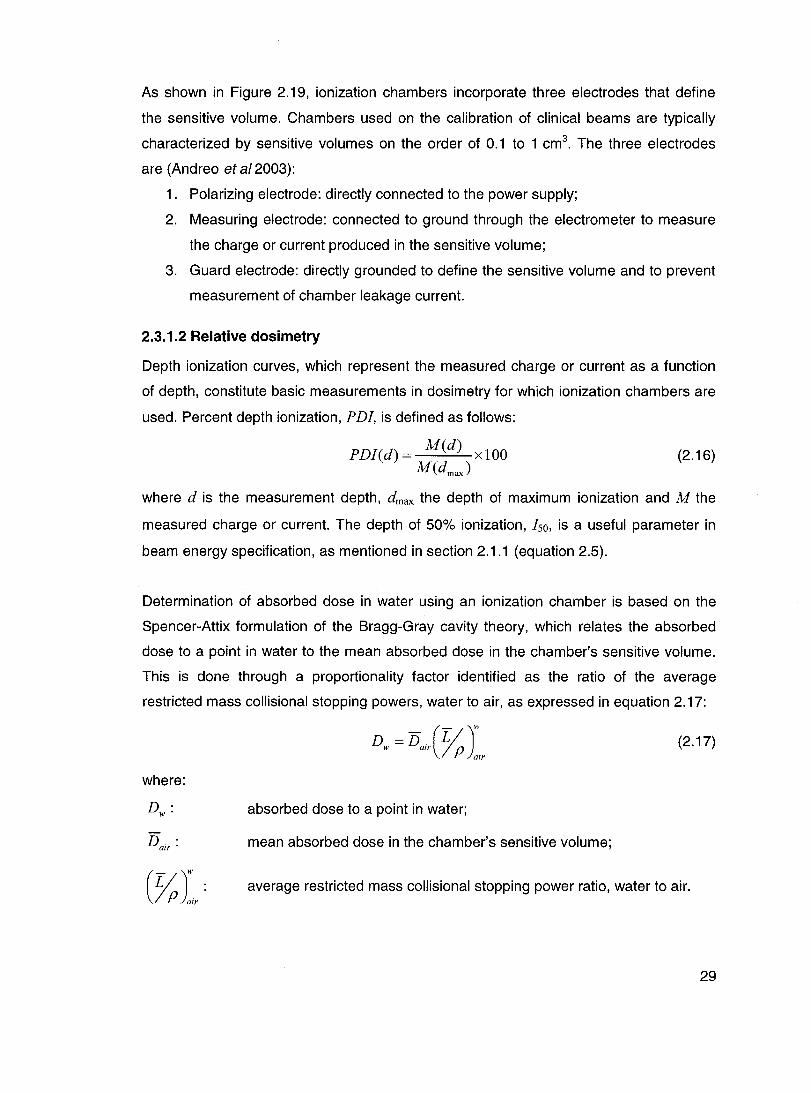
As shown in Figure 2.19, ionization chambers incorporate three electrodes that define

the sensitive volume. Chambers used on the calibration of clinical beams are typically

characterized by sensitive volumes on the order of 0.1 to 1 cm3. The three electrodes

are (Andreo et a/2003):

1. Polarizing electrode: directly connected to the power supply;

2. Measuring electrode: connected to ground through the electrometer to measure

the charge or current produced in the sensitive volume;

3. Guard electrode: directly grounded to define the sensitive volume and to prevent

measurement of cham ber leakage current.

2.3.1.2 Relative dosimetry

Depth ionization curves, which represent the measured charge or current as a function

of depth, constitute basic measurements in dosimetry for which ionization chambers are

used. Percent depth ionization, PDI, is defined as follows:

PDI(d) = M(d) xlOO M(dmaJ

(2.16)

where dis the measurement depth, dmax the depth of maximum ionization and M the

measured charge or current. The depth of 50% ionization, Iso, is a useful parameter in

beam energy specification, as mentioned in section 2.1.1 (equation 2.5).

Determination of absorbed dose in water using an ionization chamber is based on the

Spencer-Attix formulation of the Bragg-Gray cavity theory, which relates the absorbed

dose to a point in water to the mean absorbed dose in the chamber's sensitive volume.

This is done through a proportionality factor identified as the ratio of the average

restricted mass collisional stopping powers, water to air, as expressed in equation 2.17:

(2.17)

where:

absorbed dose to a point in water;

Dair : mean absorbed dose in the chamber's sensitive volume;

average restricted mass collisional stopping power ratio, water to air.

29

For electron beams, the water-to-air stopping power ratios are strongly dependent on

energy and depth because of considerable variation in energy spectra at various depths

in water. As a result, depth ionization curves obtained with air ionization chambers can

be converted to depth dose curves if corrections for the change in restricted stopping

power ratios with depth are applied. Therefore, equation 2.18 is necessary to obtain the

percent depth dose in water from ionization cham ber measurements:

(2.18)

PDD values can then be renormalized for shifts in dmax due to the conversion. Stopping

power ratio data can be found in tables or can be calculated as a function of depth using

the beam quality specifier R;o in equation 2.19 (Burns et a/1996):

where

A = 1.0752

E = -0.42806

B = -0.50867

F= 0.064627

C = 0.088670 D = -0.08402

G = 0.003085 H = -0.12460.

2.3.1.3 Calibration of high-energy electron beams

It is possible to perform the beam output calibration based on a dose-to-water cham ber

calibration coefficient from a standards laboratory. This calibration coefficient is obtained

by irradiating the cham ber in a reference beam quality, most often Cobalt-60 gamma

rays. For ail electron beams below 10 MeV nominal energy, the use of a parallel-plate

ionization cham ber is preferred and the reference medium should be water. The output

calibration should be carried out at a reference depth dref given by equation 2.20

(Almond et a/1999):

(2.20)

The absorbed dose to water at the reference depth dref in an electron beam of quality Q,

in the absence of the cham ber, is given by equation 2.21 (Andreo et a/2003):

30

where

M Q :

Po. gr·

k~ : 50

kecal :

N Co • D,w •

(2.21 )

Chamber signal corrected for influence quantities;

Gradient correction factor, unit y for parallel-plate chambers;

Electron quality conversion factor;

Photon-electron conversion factor;

Calibration coefficient in terms of absorbed dose to water for the

cham ber irradiated in a Cobalt-60 beam at standards laboratory.

Generally, the beam output is expressed at d max in a water phantom. The dose at dref

given by equation 2.21 is then converted to the dose at dmax using available POO data

for the linear accelerator of interest.

2.3.2 Radiographie films

Radiographic film dosimetry is commonly used to determine relative dose distributions of

electron beams. In clinical situations, films can be advantageous since they can be used

either in water, in plastic or in heterogeneous phantoms. Moreover, films can provide

entire two-dimensional relative dose distributions in a single irradiation. Even if the

photographic emulsion of radiographic films does not represent a homogeneous medium

with low atomic number, the short irradiation time required and the high spatial resolution

make films interesting radiation dosimeters to use in a radiation oncology clinic.

2.3.2.1 Photographie emulsion prineiple

The radiographic film is constituted by a photographic emulsion: microscopic grains of

silver halide in gelatine spread on cellulose acetate. When radiation is absorbed in a

grain, a latent image is formed after reduction of the grains to silver through chemical

development. Then, the unreacted grains are chemically removed and the reduced

grains that interacted with radiation form an image (Shani 1991, p. 117). On a uniformly

illuminated light box, exposed sections of the film are blackened, whereas non-exposed

sections appear translucent.

When a pencil light beam of intensity 10 is passed through a processed film, the optical

densityof the film (00) is defined as follows:

31

OD=lO{; ) (2.22)

where l is the intensity of the transmitted light. 00 is the quantity of interest in radiation

dosimetry since it is related to the radiation dose delivered to the film. However, there

are other factors to take into account when considering film blackening. Among others,

film type and batch, processing technique, developer temperature and fixation procedure

are ail parameters of influence. To perform reliable film dosimetry, these parameters

should be kept constant (Blais 1990, p. 21).

2.3.2.2 Dosimetry

The relation between radiation dose and the optical density of the film is described by

the sensitometrie eurve of the film, which represents the variation of net 00 as a function

of the delivered dose. Even non irradiated films show a significant 00 after processing.

This 00 is referred to as the background density. The net 00 caused by radiation is

obtained by subtracting the background density from the measured 00. The net 00 is

the quantity of interest for dosimetry. In general, a plot of the net 00 as a function of the

dose will ri se linearly from zero with increasing dose, up to a saturation region reached

at high doses. The dose ranges of the linear and saturation portions of the curve can be

different for different type of films. In film dosimetry, measurements in the saturation

region should be avoided.

A batch of films must be calibrated in order to use them as dosimeters. This calibration is

accomplished by building the sensitometrie curve of the batch. The calibration process

requires taking several films from the batch and irradiating each of them with a known

and different radiation dose, determined as precisely as possible by an absolute

dosimetry system. Then, the films are processed and the 00 of each film is measured. A

film that did not receive radiation must also be processed to determine the background

00. Net optical densities are calculated and plotted as a function of the delivered

radiation dose. The sensitometric curve obtained will be used to convert relative 00

distributions into relative dose distributions. For electron beam dosimetry, films can show

energy dependence, so calibration using the electron energy of interest for

measurements is recommended.

32

Considering the possible differences between films, the sensitometric curve (net 00 vs

radiation dose) should be measured for each type of film and for a given set of

processing conditions. According to the literature (Dutreix and Dutreix 1969), processing

conditions are not critical when relative measurements are made on the same film or on

series of films processed simultaneously, but this is not the case when films are

processed separately. Table 2.1 summarizes the uncertainty expected on relative dose

measurements using radiographic films:

Table 2.1 Expected uncertainty on relative dose measurements with films (Modified

from Dutreix and Dutreix 1969).

Measurement conditions

On the same film

On films processed simultaneously

On films of the same batch processed separately (identical processing conditions)

On films of different batches

Expected uncertainty

2%

3%

5%

Unknown

This explains why relative measurements do ne with films processed separately should

be restricted to films of the same batch.

One of the most common types of films used in radiotherapy verification is the Kodak

ready pack X-Omat-V (XV) film. These films have a high sensitivity and their response is

not linear over a wide dose range. Typically, XV films will show a linear response up to

50 cGy.

2.3.2.3 Film position with respect to beam axis direction

ln clinical situations, placing the film in a plane containing the beam axis can be most

convenient. This setup makes it possible to obtain, with a single irradiation, a full set of

isodoses in that plane. It has been observed that depth 00 curves obtained from paraI/el

or edge-on irradiations do not agree perfectly with depth curves obtained from a

perpendicular orientation. Particularly, in the region of the entrant surface of the film, an

underestimation of the absorbed dose (Iinked to differences in net 00 of about 5-10%) is

observed when the film is parallel to the beam axis. This phenomenon is attributed to the

33

increased scatter due to the high atomic number of the emulsion near the entry surface

(Dutreix and Dutreix 1969). At depth, this effect is not perceptible because of an

increase of the average scattering angle of electrons at lower energies. This

underestimation, for electron beams of nominal energies between 10 and 20 MeV, is

usually contained in the first 5 mm of the depth curve (Dutreix and Dutreix 1969).

Other complications can take place when irradiating a film in a direction containing the

beam axis. Two major precautions must be taken (Dutreix and Dutreix 1969):

1. Heavy pressure on the phantom to avoid any air gap on either side of the film;

2. Perfect alignment of the film edge with the surface.

If these conditions are not satisfied, distorsion of the depth OD curve will be observed,

as shown in Figures 2.20a, band c.

d (%) ::0 if'----.~~~

80 il! ~ 70 fi ';mm \

60 f: 50 e ~ \

40 =--. film \

20MeV~ \ .------------.'

110 1\,'· d (%) 1001f'i'o.",\'m.",...' ~=

BO

90

70 \

:: _e r:1/Z( \ 40 20 MeV vi ,1;1;; flIm \

.--, °0~----'5'-------"10'------

x (cm) o 1 2 3 4 5 6 7 8 9 10 x(cm)

o 1 2 3 4 5 6 7 8 9 10 x (cm)

(a)

Figure 2.20

(b) (c)

Film artefacts created by misalignment of the film in the phantom. The effects of (a) air gaps between the film and the phantom, (b) film edge extending beyond the phantom, and (c) film edge recessed within the phantom (Adapted from Khan 2003).

Respectively, the above figures show the impact of thin air gaps along the film surface,

of the edge of the film protruding from the phantom and of the edge of the film recessed

within the phantom.

2.3.3 Thermoluminescent dosimeters

Many dosimetry problems occurring in radiation therapy can be resolved by using

thermoluminescent dosimeters (TLD). Their small size and large range of useful dose

make TLDs a good choice to perform direct dose measurements under conditions for

which other types of dosimeters, such as ionization chambers, are impractical. Among

other clinical applications, TLDs can be used in patient dose monitoring, percentage

depth dose determination and dose monitoring in body cavities.

34

2.3.3.1 Thermoluminescence principle

The first stage of the thermoluminescence phenomenon is the perturbation of a system

from equilibrium to a metastable state. This step requires absorption of energy by the

thermoluminescent material and in the case of thermoluminescence, ionizing radiation or

UV light constitutes the external energy source. In thermoluminescence dosimetry, the

main goal is to determine the energy per unit mass of material that has been absorbed

during the irradiation process. This can be done during the second stage of the

thermoluminescence process: the thermally stimulated relaxation of the system.

The thermoluminescence phenomenon can be qualitatively explained by the

hypothetical energy diagram shown in Figure 2.21.

Figure 2.21

(a) Exposure to lonlzlng radiation.

(b) Heatlng: Electron trap is less stable, hole

trap Is the emitting center.

(c) Heating: Hole trap Is less stable, electron

trap Is the emltting center.

Schematic energy-Ievel diagram of an insulating crystal that exhibits TL due to radiation (Adapted from Cameron et a/1968).

The thermoluminescence phenomenon can take place in crystals containing defects

(impurity sites) in their crystal lattice. After absorbing ionizing radiation, electrons and

holes from su ch a crystal can get trapped in impurity sites, as shown in Figure 2.21 a.

The number of trapped electrons (holes) produced is proportional to the ionizing

radiation absorbed. Heating the crystal can lead either the electron trap or the hole trap

to be less stable than the other. As a result, the electron goes back to the conduction

band (Figure 2.21 b) or the hole goes back to the valence band (Figure 2.21 c). In both

cases, there is recombination between an electron and a hole resulting in light emission.

The temperature needed to release the electron (hole) from its trap is related to the

energy gap E.

ln practical situations, a large number of trapped electrons and holes are produced and

impurity sites are characterized by is more than one energy levaI. The probability of

35

releasing an electron (hole) is increased as the crystal is heated. During heating,

thermoluminescence starts weakly, goes to a maximum (unique for each energy level),

and then decreases to zero. This is due to the fact that, as the crystal is heated, the

probability of releasing a trapped electron (hole) increases, while the population of

trapped electrons (holes) is diminishing. This phenomenon is expressed by the glow

curve of the crystal, which is the light emitted as a function of time. The

thermoluminescence process can also be defined as a function of temperature if the

TLD heating profile function is linear. The integral of thermoluminescence as a function

of time (area under the glow curve) is proportional to the absorbed dose. Depending on

the thermoluminescent material, different peaks are observed on the glow curve, which

will be discussed in section 2.3.3.3.

2.3.3.2 Dosimetry

TLDs are relative dosimeters. In order to determine absorbed dose, they must be

calibrated against an abso/ute dosimetry system, such as an ionization cham ber. The

calibration process goes as follows: first, the TLDs are irradiated to a known dose, which

is determined by the absolute dosimetry system. Second, TLDs go through the readout

process, which consists of heating the TLDs in a systematic fashion and integrating the

glow curve over time to get the total thermoluminescence. The photomultiplying system

of TLD readers allows measured thermoluminescence to be expressed in terms of

electric charge. The given dose, D, is proportional to the measured charge, Q, and the

proportionality constant between the two is the calibration coefficient, C. For every TLD,

the calibration coefficient is determined with the following relationship:

D=C·Q. (2.23)

As long as the TLD response is linear with dose, which is usually true over a specified

dose range, the calibration coefficient is independent of the dose. If TLDs are used

beyond the linear region, a calibration curve (thermoluminescence vs delivered dose)

must be obtained to determine calibration coefficients applicable for every dose. Since

TLDs can be radiation quality dependent, it is recommended to perform calibration in

beams having a similar radiation quality to the one of interest.

One of the advantages of TLDs is that they are re-usable. However, to obtain reliable

results, it is necessary to follow a strict thermal annealing procedure, which is normally a

particular recipe of pre-irradiation annealing. This step will re-establish the

36

thermodynamic defect equilibrium that originally existed in the TLD before previous

irradiation and readout (McKeever et a/1995). The temperature, the time of heating and

the time of cooling required to optimize the dosimetric characteristics of the TLDs will

depend on the TLD mate rial. Post-irradiation annealing is also recommended but

optional. Many annealing schemes can be used, but to obtain reliable and reproducible

measurements it is crucial to always use the same recipe for a given TLD batch. To

improve precision, it is also necessary to repeat measurements or to use many TLDs for

the same measurement because thermoluminescence is a statistical process.

2.3.3.3 Characteristics of LiF :Mg,Ti (TLD-100)

ln a radiation therapy treatment, the total uncertainty on delivered dose to patients

should not exceed 5%. This means that any detector that is used to assess dose should

be as sensitive and as stable as possible. In absorbed dose determination through TLD

measurements, the method used to perform any of the previously mentioned steps has

an impact on both these characteristics. The following section details the procedure

recommended when using one of the most common TLD mate rials, LiF (TLD-100), in

order to optimize its useful dosimetric characteristics.

Figure 2.22 shows the typical glow CUNe of a LiF (TLD-100).

Figure 2.22

...J 1-.,

30

24--

.:: 16 1ii "ii Il::

8

-190"C (8O,Yr)

\

/1 [70\,'» i

(05;") 1 1 -105"'C y 1

(10 hr) / \. J

'l'V {5mln} /

r JI '\....--

Tlme (sec)

An example of glow curve of LiF (TLD-100) after phosphor has been annealed at 400°C for 1 hour and read immediately after irradiation showing 5 peaks with their respective half-lite (Adapted from Khan 2003).

After irradiation, peaks 1 through 5 decay at room temperature with the approximate

half-lives of 5 minutes, 10 hours, 0.5 year, 7 years and 80 years, respectively (Cameron

et a/1968). This makes peaks 3, 4 and 5 the most suitable for dosimetry, since they are

37

stable. Various combinations of thermal treatments can remove peak 1 and sometimes

even peak 2 from the glow curve.

Since the thermoluminescent response of TLD-100 is very sensitive to ail thermal

treatment, a general annealing procedure is recommended. Before use, the TLDs should

be submitted to a high temperature annealing of 1 hour at 400°C, followed by low

temperature annealing (80°C for 24 hours or 100°C for 2 hours). If this is not convenient

because of time constraints, only a 15 minute cooling period at a high cooling rate is

sufficient for the TLDs to keep constant sensitivity. During the readout process, a

constant heating rate is used, typicallY 5°C/s to go from 50°C to 300°C.

It should be emphasized that TLD-1 00 is considered sufficiently sensitive to enable dose

measurements down to 100 IlGy and to have a linear dose response for doses up to

1 Gy, depending on radiation quality. For higher doses, the response is supralinear up to

103 Gy and sublinear afterwards (McKeever et a/1995). However, this effect depends on

radiation quality. In terms of energy dependence, the response of TLD-100 has been

shown (Robar et a/1996) to depend on the energy of clinical electron beams, the effect

being more important at low energies. Energy dependence has also been shown to vary

with the TLD size.

38

CHAPTER 3 - MATERIALS AND METHODS

3.1 Materials

Ali measurements were performed with an Elekta SL-25 linear accelerator, using

10 MeV nominal energy electron beams. For this beam energy, dref and dmax are

respectively 2.14 cm and 2.01 cm in water for stationary beams.

3.1.1 Applicators and masks

Table 3.1 shows the different applicators and mask dimensions used during the study.

Table 3.1 Applicators and masks used in the different parts of the study.

Experiment Applicator

Oosimeter calibration Standard a

Static POO measurements Arc b

Arc irradiations Arc

Mask dimensions

20x20 cm2c

6x20 cm2c

20x20 cm2C

3x20 cm2d

6x20 cm2c

8x20 cm2d

a 5 cm between the end of the applicator and the machine isocentre;

b Arc therapy dedicated applicator; 18 cm between the end of the applicator and the machine isocentre.

c 1 cm thick masks made of a lead and aluminum al/oy;

d 1 cm thick cerrobend masks.

3.1.2 Phantoms

Water, solid water and acrylic phantoms were used throughout the study. Table 3.2

describes the phantoms related to each experiment.

For arc irradiations, in every cylindrical acrylic phantom, two sets of circular slabs were

dedicated to TLD measurements. Figure 3.1 a shows the first set of two slabs, each

1.27 cm thick, where TLDs are placed in the non-aligned configuration. This TLD

distribution allows measurement of radial PDDs, but also verification of dose uniformity

at dmax and near the surface for the totality of the arc. Figure 3.1 b shows the second set

of two slabs, both 2.54 cm thick, used only for radial PDD measurements. Holes for

39

TL Os were drilled along the central axis radius of two of the 2.54 cm thick slabs, giving

the vertically aligned configuration. A distance of 1 cm separates every TLO hole in each

plate and holes are ail shifted 0.5 cm from one plate to another so a radial POO with

points every 0.5 cm can be measured.

Table 3.2 Phantoms used in the different parts of the study.

Experiment

Oosimeter calibration

Static POO measurements

Arc irradiations

Water

Med-Tec water tank

model MT -100

WP700 Wellhôfer

water tank C

None

a Gammex RMI model 457;

Solid water a

Flat phantom of 14 cm thickness:

• 2 slabs of 2 cm; • 2 slabs of 5 cm.

Flat phantom of 19.5 cm thickness:

• 1 slab of 6 cm; • 1 slab of 4 cm; • 3 slabs of 2 cm; • 2 slabs of 1 cm; • 1 slab of 0.5 cm; • 2 slabs of 0.3 cm; • 2 slabs of 0.2 cm.

None

b Density 1. 17 g/cm3 measured by water displacement;

C Scanditronix Wellhofer.

Acrylic b


• 2 slabs of 1.8 cm; • 4 slabs of 2.5 cm.


• 2 slabs of 0.15 cm; • 3 slabs of 0.3 cm; • 2 slabs of 0.5 cm; • 1 slab of 0.6 cm; • 2 slabs of 1.25 cm; • 2 slabs of 2.5 cm; • 1 slabs of 5.0 cm.

5 cylindrical phantoms made of:

• 11 slabs of 2.54 cm thickness;

• 3 slabs of 1.27 cm thickness;

Phantom radii: • 5.1,7.6,10.2,12.7,

15.2 cm.

40

+- buildup #1

• brem #1

Figure 3.1

(a)

()

0

0

0

: t1cm

" (}

(b)

".~~~~-- .... --~ ............. "' ...

* * ...... --. .. -,-Il \~

-\ , , , 1

.. - !

-............ _-~--_ .. -..... ' "

()

0

0

0

1cmt:

"

" .' -'

~ , , :

.' ,/

• surface

* buildup#2

DR",

• brem #2

TLD plates for arc irradiations: (a) non-aligned configuration and (b) vertically aligned configuration.

One polystyrene plate (1 cm thick, 30x30 cm2) was available for TLD measurements and

referred to as the TLD calibration plate (Figure 3.2)

Figure 3.2

...--. 8.50m

300m

Calibration plate for TLDs. 50 TLD chips can be irradiated simultaneously.

41

3.1.3 Detectors

Table 3.3 summarizes ail the detectors used in the study as weil as their related reading

equipment.

Table 3.3 Detectors and related reading equipment.

Detectar

IC-10 cylindrical chamber a

NACPcal parallel-plate chamber b

NACP parallel-plate chamber a

Kodak X-Omat-V radiographie films

LiF thermoluminescent TLD-1 00 1 x1 x6 mm3 rods C

a Scanditronix We/lhOter;

b CAL CAM design trom Dosetek;

C Harshaw/Bicron.

Reading equipment

CU 500E dual processor based control unit a

Keithley electrometer model 35040 calibrated with NACPcal

Keithley electrometer model 35040

• AGFA Curix Compact Plus developer

• Wellhëfer film densitometer WP 102 a with WP700 software

• 5500 Automatic TLD reader C

with TLOshel! software

• Matlab 7.0 software

• Thermolyne Type 47900 Model F47925 Automatic TLD oven

The set NACPcal chamber/Electrometer was cross-calibrated, following AAPM TG-51

recommendations, against a clinically used Farmer type NE 2571 ionization chamber

and its dedicated Keithley electrometer, calibrated at the National Research Council of

Canada. This cross-calibration allowed the determination of Ni/w for the NACPcal

chamber.

3.2 Detector calibration

Please note that ail the following static irradiations were done at 100 cm SSD.

3.2.1 Depth scaling

Prior to performing arc measurements in cylindrical acrylic phantoms (section 3.4),

dosimeter calibration and validation in acrylic was required. It became necessary to

42

relate depths where the energy spectrum is assumed to be the same in acrylic and water

phantoms, which are called equivalent depths. The IPEM code of practice for electron

dosimetry for radiotherapy beams of initial energy from 4 to 25 Me V based on an

absorbed dose to water calibration (Thwaites et al 2003) provides a general depth

scaling method when conversion of a depth in a non-water phantom to an equivalent (or

effective) depth in water is required, or vice versa. An approximation of the effective

water depth is given by scaling the non-water phantom depth (Thwaites et al 2003):

dwater, effective = dnon-water . C pl (3.1 )

where Cpl is the depth scaling factor. Recommended values of Cp! for solid water and

acrylic are given in table 3.4:

Table 3.4 Recommended values of Cp! for solid water and acrylic (From Thwaites et

al 2003).

Phan tom material

Solid water (Gammex RMI model457)

Acrylic

Quoted standard density

[g/cm3]

1.04

1.185

Scaling factor

Cpl

1.00

1.13

If the measured density of a given sam pie of mate rial used locally is different than

quoted densities, equation 3.1 becomes:

Pnon-water

d - d .C. meas water, c:;ffective - non-wafer pl non-water

Pstd (3.2)

where p;~:~water and p;~n-water are respectively the measured and the quoted standard

densities of the non-water mate ria!.

Equivalent solid water depths in locally used acrylic were established by depth scaling

as follows:

1. Measurement of acrylic density (p;~:) and of solid water density (P:as) by

water displacement;

2. Scaling of solid water and acrylic depths (equation 3.2);

3. Obtaining depths in acrylic from depths in solid water:

43

C SW sw aery d = d . _pl_. Pmeas . Pstd

aery sw C aery sw aery pl P std P meas

(3.3)

3.2.2 NACP parallel-plate chamber calibration

The daily output of a linear accelerator can vary by up to 2%. To lower the uncertainty

level on measurements, a practical method to perform reliable and fast output

measurements was established. It consisted of finding a calibration coefficient in cGy/nC

for a NACP ionization cham ber under experimental conditions that could be precise and

reproducible every day without the need of a water tank. The following procedure shows

how to obtain the calibration coefficient for the NACP cham ber:

1. With a traceable calibration coefficient provided for the NACPcal chamber (N~~w)'

the beam output at dmax in the water phantom, following AAPM TG-51

recommendations (see section 2.3.1.3), is determined;

2. With NACP cham ber placed at dmax in the sol id water calibration phantom (table

3.2), an average collected charge from 4 irradiations of 200 MU each is obtained;

3. The calibration coefficient for the NACP chamber is calculated:

C _ D(NACPeal ) x 200 MU NACP - M

NACP

(3.4)

where

CNACP

:: Calibration coefficient for the NACP cham ber [cGy/nC];

D(NACPeal

): Beam output at dmax from NACPcal measurement [cGy/MU];

M NACp: Average collected charge from NACP measurement [nC].

Based on CNACP, the daily output of the machine at dmax in solid water (D ) is dmax

determined by repeating step 2 and using the following equation:

D - CNACP xM NACP

d max - 200MU (3.5)

44

3.2.3 Film calibration

3.2.3.1 Calibration in solid water and acrylic

Films were developed 18 hours after irradiation. In ail cases, a non-irradiated film of the

same batch was processed and used for background subtraction. Film calibration was

pertormed in both solid water and acrylic calibration phantoms (table 3.2) using the

following procedure:

1. Determination of Ddmox

with NACP chamber;

2. Positioning of the film in its ready pack envelope at dmax in the phantom,

perpendicular to the beam axis;

3. 1 rradiation of different films to the following number of MUs: 5, 10, 15, 20, 25, 50,

75,100,125 and 175 MU;

4. Film processing and net 00 measurements;

5. Dose assessment for every irradiation:

Dose d = D d • number MUs; max max

(3.6)

6. Building the sensitometric curve of the film batch by plotting the dose as a

function of the net 00.

A new sensitometric curve was obtained for every new batch of films.

3.2.3.2 Energy dependence verification

The energy dependence of X-Omat-V films in a clinical electron beam of 10 MeV

nominal energy has also been studied. The procedure consisted of film calibrations in

solid water as described above, where a sensitometric curve was determined for

different depths using the solid water phantom for static POO measurements (table 3.2).

Table 3.5 lists the different calibration depths with their corresponding approximate

electron energies, the POO values for each depth and the number of MUs delivered.

POO values come from measurements explained in section 3.3. Dose assessment

required the application of the appropriate POO value:

Dose( d) = D d • number MUs· P DD( d) . (3.7) ma,

45

Table 3.5 List of parameters for radiographie film energy dependence verification.

Calibration depth Ed a PDD

Number of MUs [cm] [MeV] ["fo]

0.8 7.4 93.6 25,50,75,100,125,150,175,200

1.5 6.2 98.1 25,50,75,100,125,150,175

2.0 5.4 100 25,50,75,100,125,150, 175

2.4 4.8 98.2 35, 70, 105, 140, 175

3.2 3.4 76.7 25,50,75,100,125,150,175,200

4.2 1.8 22.9 25,50,75,100,125,150,175,200

5.2 0.2 1.8 50,100,150,200,250,300,350,400

x-rays 7.2 1.6 100,200,300,400,500,600,700,800

:0; 10 MeV

a Calculated with equations 2.6 and 2.7 with Rso* = 3.73 cm and Rp = 5.3 cm.

3.2.4 TLD calibration

3.2.4.1 General TLD handling

Throughout the entire calibration process, TLDs were placed in the TLD calibration plate

shown in Figure 3.2. The same readout and annealing procedure was used for ail TLD

measurements. The following presents the TLD treatment 15 hours after irradiation:

1. Readout (Automatic TLD reader) with following time-temperature profile (TTP):

a. Heating from 50°C to 300°C at a rate of 5°C/s;

b. Annealing at 300°C for 5 s;

c. Cooling back to 50°C;

2. Exporting glow curve from TLDsheli to in-house deconvolution Matlab 7.0

program:

a. Deconvolution of the 5 peaks in the glow curve (Figure 2.22);

b. Subtraction of the first peak (around BO°C);

c. Calculation of total thermoluminescence (area under the curve) in

arbitrary units (a.u.);

46

3. Annealing (TLD oyen):

a. 400°C for 1 hour;

b. 15 minutes cooling between two copper plates.

Since thermoluminescence is a statistical phenomenon, the precIsion of the results

obtained with TLDs was improved by repeating the same measurements three times.

Then, it was possible to choose the most stable TLDs in a given batch, i.e. those that

showed the smaller standard deviation during calibration. Aiso note that, for ail TLD

measurements, Dd was determined with the NACP ionization chamber in a static field ma"

in solid water.

3.2.4.2 Individual TLD calibration

The following individual TLD calibration was performed, three times for each TLD:

1. Positioning of the calibration plate at dmax in the solid water phantom;

2. Irradiation of the TLDs to 200 MU;

3. Registration of total thermoluminescence (TL) for each TLD individually;

4. For each of the TLDs, calculation of (TLi )200 ' the average TL for the 3 individual

calibration readings [a.u.].

Only stable TLDs were selected to use throughout the experiments. Then, the average

of ail (TL i )200 of the batch was calculated and is referred to as (TL)200.

3.2.4.3 Non linearity correction of the dose response

ln this study, doses ranging between 50 and 900 cGy are used in electron arc

irradiations. It is weil known that TLD response is not linear over the whole dose range of

interest (Cameron et al 1968). The calibration coefficient of each TLD is dose

dependent. To obtain reliable dose measurements, a dose calibration curve,

representative of the entire TLD batch, is required in order to convert TL to dose. 50 TLD

rods were divided into 10 groups of 5 TLDs and each group was irradiated to a different

number of MUs, as shown in table 3.6. Ali TLDs were irradiated at dmax in solid water and

dose assessment was performed using the NACP cham ber for dose rate determination,

using equation 3.6. Then, the average TL for each group of 5 TLDs irradiated with a

given number of MUs, (TL):u' was calculated.

47

Table 3.6 Irradiation conditions for obtention of TLO calibration curve.

TLDs Number of MUs

1 ta 5 50

6 ta 10 150

11 ta 15 300

16 ta 20 400

21 ta 25 500

26 ta 30 600

31 ta 35 700

36 ta 40 800

41 ta 45 900

46 ta 50 989

3.2.4.4 Conversion of TL response to dose

Conversion of the measured TL to dose is based on the use of an analytical expression

representing the calibration curve, dependent on the ratio TLi /(TL)200' where TLi is the

measured thermoluminescence read for a given TLO rod. Thermoluminescence values

in this study are given in arbitrary units (a.u.).

ln every experiment, a control group of 5 TLOs (TLOs #1 to 5) was irradiated ta 200 MU

under individual calibration conditions. TL response for TLOs of the control group was

then converted to dose using a correction factor taking into account the individual

sensitivity of a given TLO, based on the individual calibration performed at 200 MU.

The second step of TL to dose conversion was dedicated to individual TL Os from the

current experiment. In addition to a correction for individual sensitivity, a correction factor

taking into account the daily sensitivity of the TLO batch and the TLO reader was also

applied, based on the behaviour of the control group. A detailed explanation will be given

in the next chapter.

48

3.2.4.5 Energy dependence verification

The energy dependence of the TLDs was studied by performing TLD calibration at

different depths in the solid water phantom for static PDD measurements (table 3.2).

Table 3.7 shows the set of parameters taken into account in this verification process:

Table 3.7 List of parameters for TLD energy dependence verification.

Calibration depth E a POO TLOs d

Number of MUs [cm] [MeV] [%]

#6 te 30 2.0 5.4 100 25,75,150,225,300

#31 te 50 4.2 1.8 22.9 75,150,225,300

a Calculated with equations 2.6 and 2.7 with R50* = 3.73 cm and Rp = 5.3 cm.

For each depth and each group of 5 TLDs, the same calibration steps were followed.

Dose assessment was done using equation 3.7.

3.3 Static POO measurements

3.3.1 ln water

PDDs in water along the beam central axis were measured using both IC-10 and NACP

ionization chambers. Continuous scans were performed over a 17 cm depth range.

Measured depth ionization data was converted to dose by applying restricted stopping

power ratio corrections according to equations 2.18 and 2.19.

3.3.2 ln solid water

PDDs in solid water were obtained with the NACP ionization cham ber, TLDs and

radiographie films. For ionization chamber and TLD measurements, detectors were

positioned at 21 different depths in a solid water phantom (table 3.2), covering a range of

depths from the surface down to 9 cm. The NACP ionization measurements were

converted to dose by applying the same restricted stopping power ratio corrections

previously indicated.

TLD measurements were performed using 3 TLDs for each depth of the PDD curve,

positioned along the beam central axis in the TLD calibration plate. 200 MUs were

delivered for every irradiation. Each data point is an average of the 3 TLD readings.

49

The POO curve was also measured with an X-Omat-V film following the procedure

described below:

1. Positioning of the film in the direction parallel to the beam axis, in its ready pack

envelope with edge aligned with phantom surface and sandwiched between

12 cm of solid water on each side;

2. Irradiation of the film to 40 MUs;

3. Film processing and two-dimensional scanning (film densitometer);

4. Extraction of central axis percent depth optical density curve and conversion to

POO using film sensitometric curve in solid water.

Please note that only the NACP chamber was used to measure POO curves for both the

standard 20x20 cm2 and the arc applicators.

3.3.3 ln acrylic

Using the same setups and procedures as for solid water measurements, POO curves

were measured in a fiat acrylic phantom with films and TLOs. The NACP ionization

cham ber and the standard 20x20 cm2 applicator were also used in the same phantom to

acquire ionization data. A corresponding depth dose distribution in water from ionization

cham ber measurements in acrylic was obtained using the depth scaling method (section

3.2.1).

3.4 Arc irradiations

3.4.1 Dosimetric measurements

3.4.1.1 Electron arc setup

Oosimetric measurements using a direct measurement method in electron arc fields

were performed. The geometric setup for electron arc irradiations is shown in Figure 3.3.

For ail arc irradiations, the center of each cylindrical phantom was positioned at the linac

isocentre. Four acrylic phantoms with different diameters were used, defining the

source-to-surface distance (SSO) as:

SSD = SAD - di. (3.8)

50

Figure 3.3

--.--""-.... = .......................................................... ..

al SAD

Geometry of an electron arc therapy technique. The arc parameters are defined as follows: di is the depth of isocentre, equivalent to the phantom radius, w is the field width defined by the light field at isocentre, a is the total arc angle and Radial POO means the POO measured along the phantom radius and the bisector of the total arc angle.

Table 3.8 presents a summary of ail experimental parameters that were used throughout

the entire dosimetric measurement process:

Table 3.8 Summary of ail experimental arc parameters used in film and TLD

measurements.

di [cm] 5.1, 7.6, 10.2, 15.2

w [cm] 3.7,7.3,9.8

60,90,120,160

Number of MUs per degree 0.5, 2, 3, 4, 5, 6, 7

3.4.1.2 Radial PDDs

Radial PDDs were measured with both films and TLDs. First, films were irradiated in the

four cylindrical phantoms according to the following procedure:

1. Cutting films in circles of radii 0.5 cm larger than the radius of the given phantom.

Positioning the film in a direction parallel to the beam axis, sandwiched between

phantom slabs with the isocentre position identified on the film. It is known from

section 2.3.2.3 that such a setup with the film protruding from the phantom

surface leads to artifacts in the buildup region (see figure 2.20b). However, this

configuration has been chosen to facilitate film positioning in a reproducible

manner and surface identification. Films were kept in their ready pack envelope

and black electric tape was used to seal ail cut edges;

51

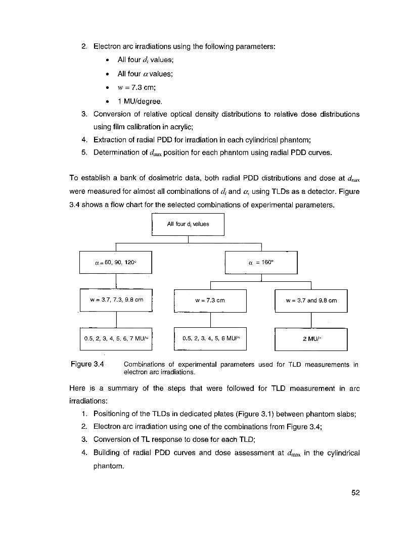
2. Electron arc irradiations using the following parameters:

• Ali four di values;

• Ali four avalues;

• w = 7.3 cm;

• 1 MU/degree.

3. Conversion of relative optical density distributions to relative dose distributions

using film calibration in acrylic;

4. Extraction of radial POO for irradiation in each cylindrical phantom;

5. Determination of dmax position for each phantom using radial POO curves.

To establish a bank of dosimetric data, both radial POO distributions and dose at dmax

were measured for almost ail combinations of di and a, using TL Os as a detector. Figure

3.4 shows a flow chart for the selected combinations of experimental parameters.

Ail four di values

1

1 1

a=60, 90,1200 a = 1600

\ 1

1 1

w = 3.7,7.3,9.8 cm w = 7.3 cm w = 3.7 and 9.8 cm

1 1 1

0.5, 2, 3, 4, 5, 6, 7 MU/o 0.5, 2, 3, 4, 5, 6 MU/o 2 MU/o

Figure 3.4 Combinations of experimental parameters used for TLD measurements in electron arc irradiations.

Here is a summary of the steps that were followed for TLD measurement in arc

irradiations:

1. Positioning of the TLDs in dedicated plates (Figure 3.1) between phantom slabs;

2. Electron arc irradiation using one of the combinations from Figure 3.4;

3. Conversion of TL response to dose for each TLD;

4. Building of radial POO curves and dose assessment at dmax in the cylindrical

phantom.

52

Ali radial POO measurements were performed down to a depth corresponding to the

isocentre in order to determine the bremsstrahlung contribution in this area. It should be

mentioned as weil that only measurements with Œ= 160° were done with TLOs in both

the non-aligned and the vertically aligned configurations.

3.4.1.3 20 dose distributions

Isodose distributions of electron arc irradiations were obtained by two-dimensional

scanning of each film acquired in the arc configuration, using the WP 102 densitometer

with a 3.0 mm spatial resolution.

T 0 verify how tertiary collimation affects the isodose distributions close to the field

edges, two different films were irradiated in an electron arc field under the following

conditions:

• w = 7.3 cm;

• 1 MU/o.

Tertiary collimation was different for each film:

Film #1: No tertiary collimation at one arc limit and lead sheets of 9 mm total

thickness covering the phantom starting on the other arc limit (Figure 3.5a);

Film #2: No tertiary collimation at one arc limit and lead sheets of 9 mm total

thickness covering the phantom starting 3 cm inside the other arc limit

(Figure 3.5b).

/Arc limits ""-

<lead_.,. )' ....

/ Arc limits ""-< L Lead sheets ... > ...... . ......... .

Figure 3.5

(a) (b)

Schematic diagram of the irradiation setup for tertiary collimation verification with films: (a) Film #1, (b) Film #2.

53

3.4.2 Predictive model for beam output

The main objective of this part of the study is to establish a practical method for beam

output determination. The method should predict how many MUs are necessary in order

to deliver the prescribed dose for a given electron arc irradiation. The method should be

simple to use and it has to be derived from the set of measured data coming from

electron arc irradiations with various di and a values. The predictive model should be

sufficiently precise in order to reproduce ail measured data within ± 3%. Moreover, it

should maintain the same level of precision for ail intermediate phantom sizes or a

values. This last feature will be tested in the model validation process.

The proposed method is based on the use of an arbitrary relationship that describes the

change of the dose rate at dmax, b;rc , as a function of di and a. For an arc irradiation max

with a given number of MUs, the absorbed dose at dmax , D;:,:, , is measured and the

corresponding dose rate is calculated as follows:

. Dd D arc =~

dmax #MU' (3.9)

The form of an analytical function was established from numerous curve fitting trials,

performed using a large number of functions applied to the same set of electron arc

beam output data. Direct comparison of calculated and measured output data for the set

of considered functions led to the selection of the most suitable one. The explicit form of

the chosen function is given in equation 3.10:

iJarc = a _ b . J~i2 ) . dmax

(3.10)

Parameters a, band c ail de pend on the total arc angle a and their relation can be

expressed as follows, using again curve fitting methods:

a = al·a+a2;

b = bl·a+b2;

loglO C = cl-c2 ·c3 Œ

(3.11 )

(3.12)

(3.13)

where al, a2, bl, b2, cl, c2 and c3 are constant model parameters. It should be

emphasized that the predictive model presented above (equations 3.10 to 3.13) was

systematically applied to the set of electron arc beam data generated with 10 MeV

54

nominal energy, the standard mask giving w of 7.3 cm at isocentre, four different

phantoms and arc angles.

To determine numerical values for ail constant parameters of the model, the following

method was applied:

1. Based on TLD measurements, registration of the dose at dmax, D are , for given dmax

phantom radius, arc angle and number of MUs;

2. Calculation of iJ;re in cGy/MU; max

3. Plot of iJ;:: as a function of (~i2) for ail available output data. Origin 7

software and equation 3.10 were used to fit the plotted data, leading to a set of

numerical values for constant parameters al, a2, b 1, b2, cl, c2 and c3.

The practical use of this predictive model is simple and straightforward. For a given

electron arc irradiation, di and a are used to calculate iJ;:.x' the dose rate at dmax ,. Then,

based on the dose at dmax prescribed bya physician, the number of MUs is calculated

with equation 3.9.

To validate the predictive ability of the model reflecting the iJ;re dependence on di and max

a, TLD measurements in dynamic electron arc fields were performed using a phantom of

different size and new arc angles. Table 3.9 shows the parameters used for this

verification.

Table 3.9 Experimental setup for verification measurements.

di [cm] 12.7

w [cm] 7.3

100, 140

Number of MUs per degree 2,6

55

The set of new measured output data was then treated in the following way:

1. Registration of the measured dose at dmax, D;eas , for a given number of MUs; ma,

2. Calculation of the measured dose rate, b;eas , using equation 3.9; ma,

3. Calculation of the corresponding fitted dose rate at dmax, bIit , using the ma,

predictive model;

4. Comparison between b meas and b fit .

dm~ dm~

Although preliminary, additional work was carried out on the effect of the field width w on

the dose rate at dmax • TLD measurements involving ail cylindrical phantoms and a = 1600

were performed. Three different field widths at isocentre were used: w = 3.7, 7.3 and

9.8 cm. Then, plots of b;rc as a function of w were built with the intent to establish a ma'

relationship between these two variables. As future work, it is planned to introduce the

field width effect on the electron arc beam output into the predictive model.

56

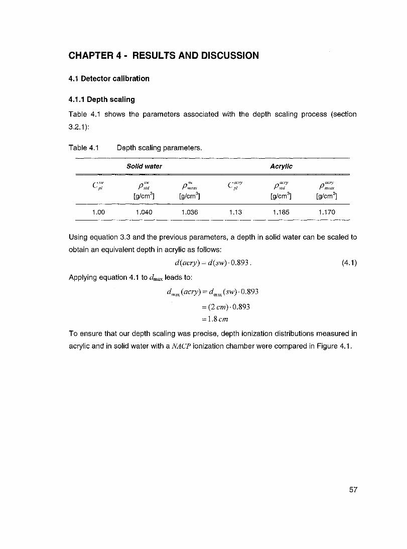
CHAPTER 4 - RESUL TS AND DISCUSSION

4.1 Detector calibration

4.1.1 Depth scaling

Table 4.1 shows the parameters associated with the depth scaling process (section

3.2.1):

Table 4.1

Csw pl

1.00

Depth scaling parameters.

Solid water

P:t~ sw

Pmeas

[g/cm3] [g/cm3

]

1.040 1.036

Acrylic

C acry pl

pacry std

pacry meas

[g/cm3] [g/cm3

]

1.13 1.185 1.170

Using equation 3.3 and the previous parameters, a depth in solid water can be scaled to

obtain an equivalent depth in acrylic as follows:

d(aery) = d(sw)· 0.893.

Applying equation 4.1 to dmax leads to:

dmax (aery) = dmax (sw)· 0.893

= (2 em)· 0.893

=1.8em

(4.1 )

To ensure that our depth scaling was precise, depth ionization distributions measured in

acrylic and in solid water with a NACP ionization chamber were compared in Figure 4.1.

57

Percent depth ionization curves 10 MeV - SSD 100 cm - 20 x 20 cm2

120,---------------------------------------------~

80

.... ~ f... 60 ëi a..

40

20

0

120

100

80

.... ~ CI 60 CI a..

40

20

0

Figure 4.1

0 2

. ....-. .. ~"'...... ,.

•

0 2

• • Acrylic

'" Solid water

•

•

• • 4 6

Depth [cm]

(a)

Percent depth dose curves in water 10 MeV - SSD 100 cm - 20 x 20 cm2

~

8

'" Measured in solid water

•

4

'" •

•

• Measured in acrylic

6 Depth [cm]

(b)

• 8 10

•

10

12

(a) Central axis percent depth ionization curves in acrylic and in solid water; (b) Central axis depth dose curves. Triangles (~) represent direct measurements in solid water. Diamonds (+) represent measurements in acrylic with equivalent depth correction fram acrylic to solid water. Ali measurements were performed with a 10 MeV electron beam, 20x20 cm2 field and SSD 100 cm using a NACP ionization chamber.

58

Figure 4.1 a shows differences in central axis depth ionization distributions between

measurements in solid water and in acrylic. This was expected since the density and the

effective atomic number of acrylic are different from those of sol id water. Then, a

correction factor of 1/0.893 (from equation 4.1) was applied to depth values associated

with measurements in acrylic to transform them into equivalent depths in solid water.

lonization data was then converted to dose using stopping power ratio corrections

previously described for water and the new corresponding depth values. The result of

this correction is shown in Figure 4.1 b. The corrected depth dose distribution (depths in

acrylic to depths in solid water) agrees with the depth dose distribution measured directly

in solid water, which means that the applied depth scaling factor is reliable.

4.1.2 NACP ionization chamber

As mentioned in section 3.2.2, an NACP ionization chamber was calibrated in a precise

experimental setup to provide a quick assessment of the Iinac output. The calibration

coefficient, CNACP, was determined from measurement and is given in table 4.2:

Table 4.2 Calibration coefficient for the NACP parallel-plate ionization chamber

used in daily output measurements.

CNACP [Gy/nC] Uncertainty [%]

0.1388 0.6

Considering the 0.6% uncertainty on the calibration coefficient and an average standard

deviation of 0.5% on the ionization readings combined in quadrature, this leads to a

relative uncertainty of 0.8% on the absorbed dose at dmax and it will be used throughout

the experiment.

4.1.3 Films

4.1.3.1 Film calibration curve

The sensitometrie curve for a given batch of X-Omat-V films in sol id water is shown in

Figure 4.2.

59

200

180

160

140

>: 120 (!)

.E. 100 (1) 1/1 0 80 c

60

40

20

0 '" 0

Figure 4.2

60

Sensitometrie eurve of X-Omat-V films

10 MeV - SSO 100 em - 20 x 20 cm2

~ :: "- 0.9971 ;7 " ,,1 & OZ 1 u"~ •• m.'$. il: 20 :: calibration ~ j~ ;?I

'"

0.5 1.5

netOD

'"

'" '"

1 2 3 4 5

net 00

Sensitometrie eurve for X-Omat-V films performed in a 10 MeV eleetron beam in solid water at depth of dose maximum dmax(sw)=2 em with a 20x20 em2 field and SSD 100 em. The inset represents a limited part of the sensitometrie eurve (net OD from 0 ta 2) and a linear relationship is fitted through the data points. The uneertainty on the dose is ineluded in the size of the dots.

Throughout the experiment, an absolute uncertainty of 0.02 on the net 00 values is

considered since it takes into account an uncertainty of 0.01, which stems from the film

densitometer, according to the technical specifications. This uncertainty is applied to

both the background and the film of interest 00 measurements.

From Figure 4.2, it is seen that the relationship between the net 00 and the dose is not

linear over the entire calibration dose range. The inset shows the linearity of the

response for doses up to 50 cGy. However, for higher doses, which are likely to be used

in clinical situations and certainly in electron arc irradiations, the sensitometrie curve has

to be applied to correctly convert relative 00 distributions to relative dose distributions.

This sensitometrie curve is applied to every film distribution using the WP 102 film

densitometer software, which performs linear interpolation between the points.

ln order to obtain more realistic results for electron arc irradiations, a sensitometrie curve

for X-Omat-V films was also built from measurements in an acrylic phantom and it is

60

shown in Figure 4.3. The comparison between calibrations in acrylic and sol id water is

also presented.

200

180

160

140

';:: 120 (!) (.)

-100 (1) III 0 80 c

60

40

20

0 0

Figure 4.3

Comparison between acrylic and solid water film calibrations

10 MeV - SSD 100 cm - 20 x 20 cm2

.. ..

" Il

1

• Acrylic

.6. Solid water

.. III

" III

2

net OD

.. Il

.. Il

3 4 5

Comparison between sensitometrie curves of X-Omat-V films pertormed at dmax in acrylic and in solid water for the same irradiation conditions: 10 MeV, 20x20 cm2

, SSD 100 cm. The uncertainty on the dose is included in the size of the dots.

Both calibrations are performed at equivalent depths, according to the depth scaling

method. Differences of the order of 6% for a dose of 125 cGy show that it is relevant and

necessary to have a special sensitometrie curve for film irradiations in acrylic.

4.1.3.2 Film energy dependence verification

The last step in film calibration was verification of the energy dependence of X-Omat-V

films in electron beams of energies of 10 MeV and lower. In Figure 4.4, the uncertainty

on net 00 measurements was included in the size of the dots to avoid visual confusion.

Please note that the dots are not representative of the uncertainty on the dose, which is

in general smaller. It is shown that, taking into account the uncertainty on net 00 values,

no significant differences appear in the calibration performed at different energies, in the

electron energy range from 3.4 to 7.4 MeV and for x-rays of 10 MeV and lower. For

energies of 0.2 and 1.8 MeV, differences appear in the net 00 as compared to the

61

calibration at the reference depth (5.4 MeV). The inset shows that, for calibration

performed at low energy (0.2 MeV), differences of the order of 10% relative to the

reference calibration occur for doses around 5 cGy. The energy dependence of these

films thus seems significant in the low energy region, close to the electron practical

range.

200

180

160

140

>: 120 (!)

~ 100 (1) CIl

~ 80

60

40

20

30

25

~ 20 u ~ 15 ., :; 10 0

5

0 0

Energy dependence verification - X-Omat-V films

10 MeV - SSD 100 cm - 20 x 20 cm2

)41 ..

l"d=20C~1 .. • +d= 5.2 cm .. " • ..

/ .. ~+++ • .. -; ++

+

.. x 0.5 1 ~. • d = 0.8 cm (7.4 MeV) net 00

• d = 1.5 cm (6.2 MeV) ,;." .. d = 2.0 cm (5.4 MeV)

~

" x d = 2.4 cm (4.8 MeV)

.~ " d = 3.2 cm (3.4 MeV)

" 0

o d = 4.2 cm (1.8 MeV) x 0

+ d = 5.2 cm (0.2 MeV) ~~ -cr" - d = 7.2 cm (x-rays)

:.. ... #++. o o

Figure 4.4

4.1.4 TLDs

1 2 3 4 5

net OD

Sensitometrie eurves of X-Omat-V films measured at different depths in a solid water phantom for a 10 MeV beam, 20x20 em2 mask, SSO 100 em. The uneertainty on net 00 measurements was ineluded in the size of dots.

4.1.4.1 Individual TLD calibration

Following the series of TLD irradiations of 200 MU in reference conditions, an average

TL value, (TL;)200' was established for each TLD in order to account for its individual

response. The maximum standard deviation on (TL;)200 for the 71 TLDs of the batch

was of 3.0%. The value of (TL)200' the average of ail (TL;)200' was also obtained:

(TL)200 = 283 ± 6 a.u.

62

The ove rail (TL)200 variation is ± 2.1%.

4.1.4.2 Non linearity correction of the dose response

As mentioned previously, groups of 5 TLDs were irradiated to different number of MUs,

giving an average value for each group, (TL):u' Then, based on (TL):u' the

corresponding TL response of the whole TLD batch to the same number of MUs,

(TL)MU' was extrapolated following equation 4.2:

(TL) = (TL)gr x (TL)200 MU MU (TL)gr '

200

(4.2)

where (TL)~~o is the average TL of the same group of 5 TLDs from the individual

calibration at 200 MU.

1200

1000

800 ->. (!) .2. 600 4) III 0 c

400

200

o

Figure 4.5

o

Calibration curve of the TLD batch

10 MeV· SSD 100 cm· 20 x 20 cm2

Y = -4.74686x2 + 208.81495.x

R2 = 0.99986

(TL}MU x=--

(TL},oo

y = Dose [cG)! 1

• d = 2 cm

- Polynomial (d = 2 cm)

2 4 5 6

Calibration curve for the whole TLD batch, performed at dmax. The uncertainty is included in the size of the dots.

The calibration curve of the TLD batch is shown in Figure 4.5, with the corresponding

analytical expression in the inset. In order to apply an appropriate correction for the

individual sensitivity of each TLD, a relationship between the group calibration and the

63

individual calibration performed at 200 MU was necessary. This relationship was found

by using the constant parameter (TL)200 to normalize ail (TL)MU values of the calibration

curve. Then, dose was plotted as a function of the variable (TL)MU I(TL\oo and an

analytical relationship was fitted through the data points. The uncertainty on (TL)MU is

calculated from the uncertainty on (TL):u' which is the standard deviation on the

response from the 5 TLDs constituting one group.

4.1.4.3 Conversion of TL response to dose

Firstly, for TLDs of the control group, TL response was converted to dose according to

equation 4.3:

Dtontrol =[-4.74686'( TL; J2 +208.81495.( TL; J~x (TL)200 , (4.3) (TL)200 (TL)200 J (TL;)200

where tL~,", is the correction factor taking into account the individual sensitivity of a TL; 200

given TLD, obtained from the individual calibration at 200 MU. Numerical coefficients

come from the curve fitting equation in Figure 4.5.

The dose associated with each TLD of the experiment is given by equation 4.4:

DTLD =[-4.74686'[ TL; J2 +208.81495'[ TL; Jlx (TL)200 X Ddmax , (4.4)

1 (TL)200 (TL)200 J (TL;)200 (DtOntrol)

where

(Dt°ntrol) :

D . dmax •

is the correction factor taking into account the daily sensitivity of the TLD

batch and the TLD reader;

is the average of DtOntrol for the 5 TLDs in the control group;

is obtained with NACP measurements.

For each TLD of a given experiment, the uncertainty on the TLD dose is calculated using

the partial derivatives method, taking into account the uncertainty on D ,/ Deontrol) , dma... \ l

64

4.1.4.4 TLO energy dependence verification

350

300

250

-~200 (.) .... CI)

~ 150 c

100

50

0 0 0.2

Energy dependence verification - TLDs 10 MeV - SSD 100 cm - 20 x 20 cm2

• d = 2.0 cm (5.4 MeV)

:t: d = 4.2 cm (1.8 MeV)

0.4 0.6

t---+-I HIH

0.8

<TL>/<TL>200

1 1.2 1.4 1.6

Figure 4.6 Calibrations at dmax and at d=4.2 cm. The uncertainty on the dose is included in the size of the dots.

Figure 4.6 shows the comparison between calibrations performed at two different depths

in order to verify the energy dependence of the TLO response. Uncertainty accounted

for, no significant differences in TL may be noted in the energy range of interest. This

feature will be evaluated and discussed in more detail in the section describing POO

data (section 4.2).

4.2 Static POO measurements: film and TLO reliability

4.2.1 ln water and solid water

The main goal of static POO measurements was to establish the reliability of films and

TLOs in electron fields by comparing obtained results to the corresponding ionization

chamber measurements. Figure 4.7 gives a summary of ail static POO measurements in

water and in solid water for electron irradiation under the same conditions.

65

100

80

-?f!. 60 ..... 0 0 D..

40

20

o o

Figure 4.7

Detector validation - Static PDDs 10 MeV - SSD 100 cm - Arc applicator with 6 x 20 cm2 mask

-IC-10 water

............. NACPwater

t:,. NACP solid water

-- Film X-Omat-V solid water

0 TLDs solid water

2 3 4 5 6 7 8 9 10 11 12

Depth [cm]

Static PDDs in water and sol id water measured with different detectors using 10 MeV nominal energy, arc applicator with a 6x20 cm2 mask and SSD 100 cm. Error bars are associated with TLD measurements.

TLO measurements agree with ionization cham ber measurements, within the margin of

error, for ail depths. This shows that the energy dependence of TLOs in electron fields,

as shown in Figure 4.6, is not a concern in this study when measuring depth dose

distributions. In the build-up region, from the surface down to 1 cm, film measurements

are not reliable. Because of the parallel orientation of the film, underestimation of the

dose from increased scatter due to the high atomic number of the emulsion occurred at

the entrant surface (section 2.3.2.3). As expected from film energy dependence

verification, a discrepancy between film and ionization chamber measurements is

observed, starting at depths greater than 4 cm. The maximum difference is observed at

a depth of 5 cm and is less than 3%.

4.2.2 ln acrylic

Since ail arc irradiations were performed in acrylic phantoms, the agreement between

TLOs and film in an acrylic phantom was checked by comparing static POO

66

measurements in a fiat acrylic phantom with both types of detectors. Figure 4.8 shows

the comparison between the two PDDs.

Figure 4.8

Comparison between statie PDDs in aerylic 10 MeV - SSD 100 cm - Arc applicator with 6 x 20 cm2 mask

Static POO in a fiat acrylic phantom measured with TLOs and X-Omat-V film using 10 MeV nominal energy, arc applicator with a 6x20 cm2 mask and SSO 100 cm. The uncertainty on the TLO position (depth) is included in the size of the dots.

It is clear from this figure that dose measurements with both detectors are practically the

same at ail depths, except in the build-up region where film fails due to its orientation.

4.3 Arc irradiations

4.3.1 Dosimetric measurements

4.3.1.1 Radial PDDs

Radial PDDs constitute an important part of the dosimetric data required for electron arc

irradiation treatments. Figure 4.9 shows a comparison of two radial PDDs for the same

arc irradiation, measured with film and TLDs. This figure is representative of the film

behaviour for the majority of the arc irradiations that were performed.

67

100

80

-<:ft. 60 .... Q Q Il..

40

20

o o

Figure 4.9

1

Comparison between electron arc radial PDDs 10 MeV - rli = 10.2 cm -w = 7.3 cm - a = 1600

\ ~ + TLDs

\

I\ --Film X-Omat-V

\ \ ,

\

. ...

2 3 4 5 6 7 8 9 10 11 12 Depth [cm]

Radial PDD measured with TLDs and X-Omat-V film in an electron arc irradiation using 10 MeV nominal energy, arc applicator with a 6x20 cm2 mask and SSD 100 cm. The uncertainty on the TLD position (depth) is included in the size of the dots.

ln the build-up region, the film underestimates the dose. This result was expected since

films were irradiated in a direction parallel to the beam axis. Furthermore, the shape of

the film POO in that region clearly demonstrates the effect of the film protruding from the

phantom surface, as previously shown in Figure 2.20b. Beyond the build-up region,

down to the depth of 4 cm, radial POOs measured with film and TL Os show reasonable

agreement. Oeeper in the phantom, the dose, measured with film, is overestimated by at

most 8% at the depth of 5 cm. Oiscrepancies between TLO and film measurements can

be explained by the fa ct that the energy spectrum of arc irradiations differs from the

spectrum of static field irradiations at the same depth in a fiat phantom. It should be

emphasized that such overestimation of dose in film measurements was not seen in

static irradiations. The situation improves in the bremsstrahlung region, where a 2%

overestimation from film measurement is observed, as in static irradiations. Clinically,

68

such discrepancies at depths greater than 4 cm are not negligible. In order to use film as

a method of clinical verification, these discrepancies must be accounted for.

Radial POOs for the same beam, measured with TLOs in two different configurations

(Figure 3.1), have been compared, as shown in Figure 4.10.

100

80

-~ 60 c C Il.

40

20

a

Figure 4.10

Radial POO measured with TLOs placed in different configurations

10 MeV - fli = 10.2 cm -w = 7.3 cm - a = 1600

a

! 1:

1

i

2

..

3 4 5

• non-aligned configuration

o vertically aligned configuration

6 7 8 9 10 11 12 Oepth [cm]

Radial PDDs measured with TLDs in an electron arc irradiation with di=10.2 cm, w=7.3 cm and a=160° for both TLD configurations. The uncertainty on the TLD position (depth) is inc/uded in the size of the dots.

For a total arc angle of 160°, both TLO configurations give the same POO. This means

that, under these irradiation conditions and particularly for these electran energies, the

influence of one TLO on another is not of concern when they are separated by 1 cm,

even if they are vertically aligned in the beam. This also confirms that, for large avalues,

the unaligned configuration is suitable even if TLOs do not lie exactly along the beam

central axis. For small a values such as 60°, a slight underestimation of dose is caused

by the fact that, in the unaligned configuration, TLOs in the build-up region are 15° away

fram the central axis. This effect will be discussed in more detail.

69

Effect of di

The influence of di on radial PDDs and on the dose at dmax has been studied. For fixed

field width and total arc angle, radial PDDs in cylindrical phantoms of different radii are

compared in Figure 4.11, which is a representative sam pie of ail similar measurements

that were performed.

100

80 J

.... 'èf!. 60 -c c D...

40

20

0

0

Figure 4.11

B

ri! 1-!lE II:

"1-

Il j[

li; ~

+

2 4

Radial PDDs measured with TLDs

10 MeV - w = 7.3 cm - a = 1600

2 MU/de ree

• di = 5.1 cm

• di = 7.6 cm

l> di = 10.2 cm

o di = 15.2 cm

+ l' <> .. .. t. ...

6 8 10 12

Depth [cm]

... ~

14 16

Radial PDDs measured with TLDs for a fixed w of 7.3 cm, a=160° and varying di values. The uncertainty on the TLD position (depth) is included in the size of dots.

The variation of the isocentre depth in electron arc irradiation was expected to influence

the surface dose and the position of dmax• From this figure, it is seen that the surface

dose increases for larger di values. This behaviour is similar to static irradiations, where

higher surface dose is obtained when the phantom is closer to the applicator. A slight

shift in the position of dmax with varying di is observed. Values of dmax for each radius of

curvature are presented in table 4.3. The positions of dmax were first determined using

films and then confirmed using both TLD configurations.

70

Table 4.3 Values of depth of maximum dose in acrylic for each cylindrical phantom,

for a=160° and w=7.3 cm.

di [cm] dmax [cm]

5.1 1.9

7.6 2.0

10.2 2.1

15.2 2.2

Our results are comparable to the British-Columbia team's. They observed sm ail

variations in the position of dmax with varying isocentre depth under similar irradiation

conditions (short electron applicator as secondary collimation, field widths of 2, 5 and

10 cm and radii of curvature in the range 10 to 17.5 cm). The McGili te am also observed

a shift of the depth of maximum dose to greater depths for larger di (Pla et al 1988).

However, they measured a 1 cm shift in dmax when di changed from 5 cm to 10 cm, for a

field width of 7 cm (Figure 2.12). It should be mentioned that the geometric setup used

by the McGili team differs from ours since they did not use an applicator as secondary

collimator. Our results show only a 2 mm shift in dmax for approximately the same change

in arc conditions.

Beyond dmax, the depth dose is not significantly influenced by the value of di, for a field

width of 7.3 cm. Variations of the therapeutic range were found to be similar to variations

of dmax• No significant variation in bremsstrahlung contribution at the isocentre was

established as a function of di.

Even though radial PDDs remain similar while varying di under the previously described

conditions, Figure 4.12 shows that the arc dose for depths down to the electron practical

range is greatly affected by the isocentre depth. It is clear from this figure that a much

lower beam output is measured for larger phantoms.

71

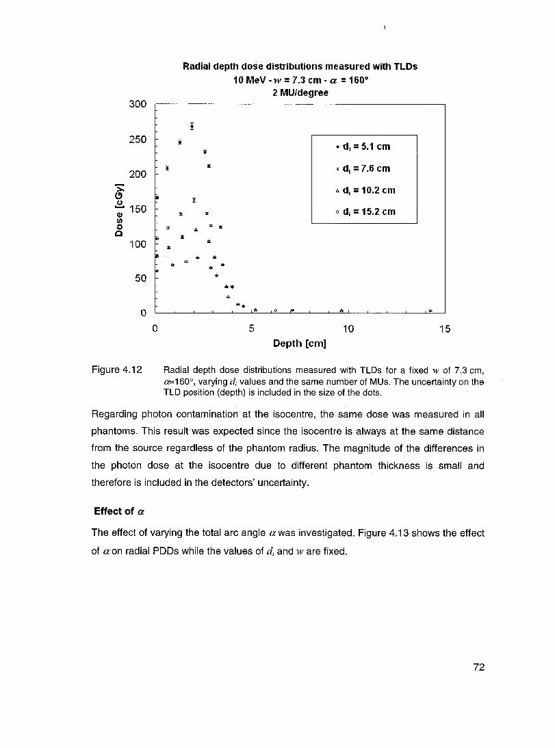
300

250

200 .... >. e" (..) .... 150 CI) /1) 0 Cl

100

50

0

0

Figure 4.12

~

:z:

li;

..

~

li:

Radial depth dose distributions measured with TLDs 10MeV-w=7.3cm-a =160·

2 MU/degree

f

~ • di = 5.1 cm

., x di = 7.6 cm

6. di = 10.2 cm l

:z: o di = 15.2 cm

A :r; •

A li;

... i!i

'" '" ... .... .;. ...

.!t <l-

5 10 Depth [cm]

15

Radial depth dose distributions measured with TLDs for a fixed w of 7.3 cm, a=160°, varying di values and the same number of MUs. The uncertainty on the TLD position (depth) is included in the size of the dots.

Regarding photon contamination at the isocentre, the same dose was measured in ail

phantoms. This result was expected since the isocentre is always at the same distance

from the source regardless of the phantom radius. The magnitude of the differences in

the photon dose at the isocentre due to different phantom thickness is small and

therefore is included in the detectors' uncertainty.

Effect of a

The effect of varying the total arc angle a was investigated. Figure 4.13 shows the effect

of a on radial PDDs while the values of di and w are fixed.

72

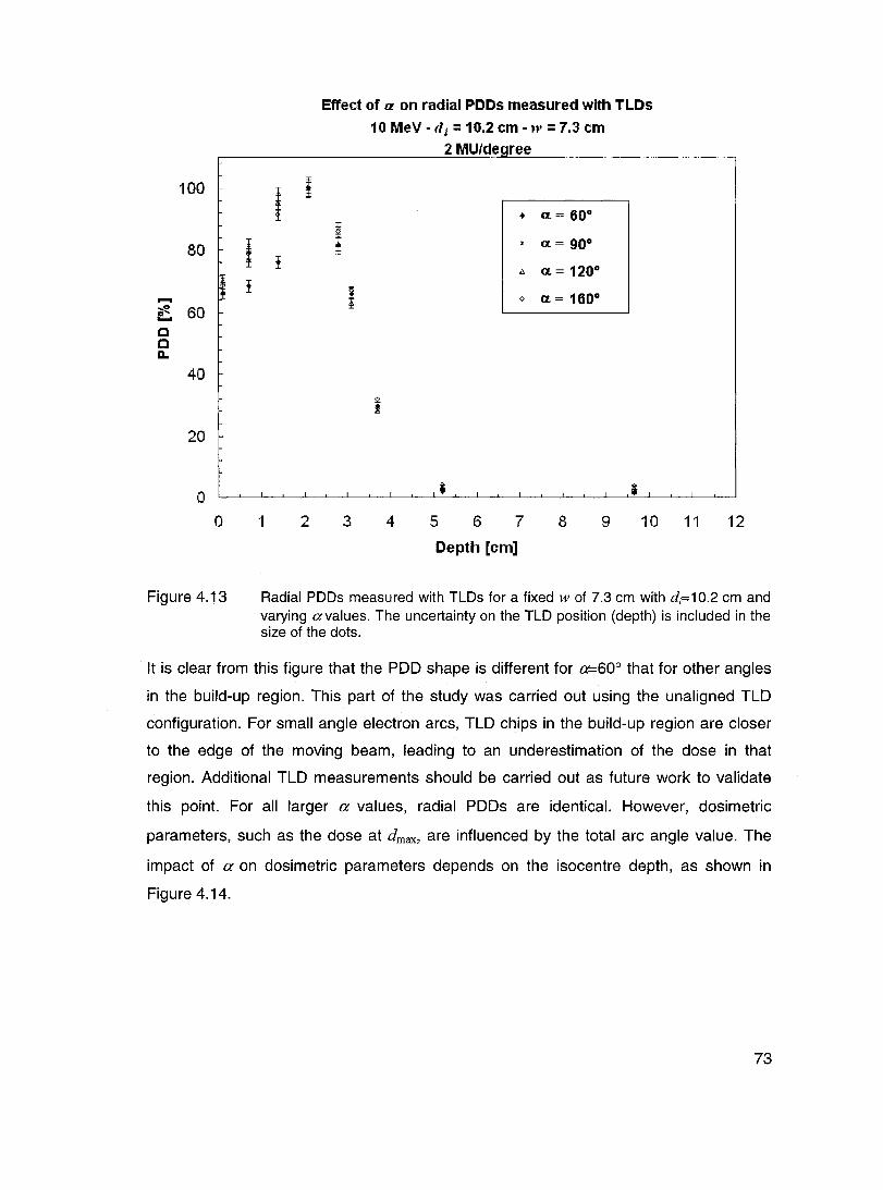
100

80 ! ! -~ 60

c C D..

40

20

o o

Figure 4.13

l ;

!

1 2

Effect of a on radial PDDs measured with TLDs

10 MeV - fli = 10.2 cm -w = 7.3 cm 2 MU/de ree

• Œ= 600

1 . Œ= 900

1:. Œ = 1200

! 0 Œ = 1600

3 4 5 6 7 8 9 10 11

Depth [cm]

12

Radial PDDs measured with TLDs for a fixed w of 7.3 cm with di=1 0.2 cm and varying avalues. The uncertainty on the TLD position (depth) is included in the size of the dots.

It is clear from this figure that the POO shape is different for a=60° that for other angles

in the build-up region. This part of the study was carried out using the unaligned TLO

configuration. For small angle electron arcs, TLO chips in the build-up region are closer

to the edge of the moving beam, leading to an underestimation of the dose in that

region. Additional TLO measurements should be carried out as future work to validate

this point. For ail larger a values, radial POOs are identical. However, dosimetric

parameters, such as the dose at dmax, are influenced by the total arc angle value. The

impact of a on dosimetric parameters depends on the isocentre depth, as shown in

Figure 4.14.

73

300

250

200

->0-C) (,)

-150 .. 1'$ E

C

100

50

o 50

Figure 4.14

Dose at dnwr. as a function of a

10 MeV"w = 7.3 cm 2 MU/de ree

• di = 5.1 cm

• di = 7.6 cm

t.d i =10.2cm

o di = 15.2 cm !

l l

.. •

70 90 130 150 170

Dose at dmax measured with TLDs for every di and a value, for a field width w=7.3 cm.

From this figure, it is seen that the effect of Œ on the dose at dmax is important for small

size phantoms (e.g. di=5.1 cm) and absent for large size phantoms (e.g. di=15.2 cm).

This effect can be explained geometrically by Figure 4.15. Let's consider an arc

irradiation as a sum of multiple beams delivered at different gantry angles with small

increments. For small radii of curvature (on the left), a point at dmax receives

contributions from ail beams of the complete arc, even for large Œ values. For larger radii

of curvature (on the right), beams constituting the entire arc contribute to the dose at

d max only up to a limit Œ value, Œ/imi!. This angle is somewhat analogous to McGill's

characteristic angle p, except that the matching point is not at the surface. When the

beams are delivered at an angle greater than Œlimit, no significant dose is added at dmax.

The value of ŒUmit is different for every radius of curvature, getting larger as the phantom

diameter is smaller. According to our results, Œlimit is smaller than 60° for di of 10.2 and

15.24 cm. For di = 7.6 cm, Œ/imit is around 90°, whereas it is over 160° for di = 5.1 cm.

74

Figure 4.15

alimil ~

Schematic diagram explaining the effect of aon the dose at dmax for different di values.

Photon contamination

Measured radial PDDs were used to establish the bremsstrahlung contribution to the

isocentre for electron arc irradiations. For ail measurements, the field width was always

kept constant at w=7.3 cm. Table 4.4 presents the photon contamination values

obtained under the given conditions.

Table 4.4 Values of the bremsstrahlung contribution at the isocentre, PDDx, from

electron arc irradiations of a= 1200 with w = 7.3 cm. Measurements were

done with TLDs at the isocentre.

MU/degree PDDx [%]

di =5.1 cm di =7.6 cm di = 10.2 cm di = 15.2 cm

0.5 3.5 2.3 3.2 3.3

2 3.5 2.1 3.7 3.4

3 3.4 2.3 2.8 3.2

4 3.3 2.0 2.5 3.5

5 3.2 2.0 2.5 3.3

6 3.0 1.9 2.7 3.1

7 3.0 1.9 2.4 3.1

75

For a 10 MeV nominal energy and a w of 7.3 cm, the bremsstrahlung at the isocentre is

always lower than 4% of the maximum dose. This level of photon contamination is much

lower than what was previously reported for a Clinac 18, e.g. 15% with a 15 MeV

nominal energy (Pla et a/ 1989). However, it should be mentioned that the conditions

leading to 15% contamination are not used clinically by the McGili team. Contamination

is maintained lower than 4% for clinical cases. In Elekta SL-25 linacs, the dual scattering

foil system is used to generate clinical electron beams, resulting in such low photon

contamination. Clinically, it makes the SL-25 linac very suitable for electron arc

treatments under the selected conditions (field width and energy).

It was previously mentioned that the absolute dose at the isocentre was the same, taking

the uncertainty into account, for ail phantoms in the same irradiation conditions. Since

the dose at dmax is higher for smaller di values, we would expect the PDDx value to

become larger as the phantom radius gets larger. This behaviour is observed (table 4.4)

for di values going from 7.6 to 15.2 cm, but the photon contribution relative to the dose at

dmax is larger for di = 5.1 cm. This is due to the fact that, for this phantom, there are still

electrons contributing to the dose at the isocentre position since it is still within the

electron practical range.

Effect of w

Increasing the field width causes an increase in the surface dose and a shift of dmax to

shallower depths, for di values of 5.1 and 7.6 cm (Figure 4.16a and b). The same

observations were also reported by Pla et a/1988. For larger di values su ch as 10.2 and

15.2 cm, there is no clear evidence of the same behaviour (Figure 4.16c and d). For the

larger phantoms, the effect of the field width on the photon contamination is clearly

observed. As expected, the bremsstrahlung contribution at the isocentre is greater for

smaller fields due to the forward peaked nature of the photon distribution. In the worst

case in our set of experimental conditions (di = 15.2 cm and w = 3.7 cm), the photon

contamination reaches 8% of the maximum dose (Figure 4.16d).

76

120

100 + + '" ...... +

~ 80 ...... C 60

x ....

c :.... Il..

40

20

a 0

120

100 • • ,. 1

;;;i' 80 ~ 1 ...... C 60 C D.. 40

20

0 0 2

Figure 4.16

Effeet of field width on radial PDDs 10 MeV - a=160°

2 MU/degree

~ .... '" .... + + M

'" .... +w= 9.8 em + '" .... +w= 9.8 cm '" ; .... +

*' '" w=7.3em .... >:w=7.3cm + .... w= 3.7 cm ... ....w= 3.7 cm

'" >: ....

d;=5.1 cm + + .... d;= 7.6 cm

>: >: + +

.... ~ ..... • .a ~ ~~~~~ .

2 3 4 5 a 2 4 6 8

Depth [cm] Depth [cm]

(a) (b)

• . .... +w= 9.8 cm • 1· w = 7.3 CI~ 1 , ~w= 7.3clI1 • w= 3.7em .... w=3.7clI1 .. + • di = 10.2 cm di = 15.2 cm

• • +

.... • • • t • • t • t t t t t + : .

4 6 8 10 0 5 10 15 20

Depth [cm] Depth [cm]

(c) (d)

Radial PDDs measured with TLDs for 0:=160° and varying w values. (a) di=5.1 cm; (b) di=7.6 cm; (c) d;=10.2 cm; (d) d i=15.2 cm.

The field width, as in any electron irradiation, greatly influences the output at dmax in the

phantom. This will be discussed further in section 4.3.2.

4.3.1.2 20 dose distributions

X-Omat-V radiographie films were used in arc irradiations to obtain full two-dimensional

dose distributions inside the phantoms. The main disadvantage of using this type of film

is the low saturation dose, making them unsuitable for simultaneous irradiation with

TLOs in electron arc fields. However, they proved to be reliable for the needs of this

study, particularly to provide qualitative 20 information.

77

0

1

2 E ~3 ..c +-' a. U) 4 0

5

6

-5

0

2

4 E ~ 6 ..c ...... a. U) 8 0

10

12

Figure 4.17

Isodose maps measured with X-Omat-V films 10 MeV - w=7.3 cm - a=160°

d,=5.1 cm Isodose [%]

-4 -3 -2 -1 0 1 2 3 4 5 Off-axis distance [cm]

(a)

d,=10.2 cm Isodose [%]

-8 -6 -4 -2 0 2 4 6 8 Off-axis distance [cm]

(b)

Comparison of isodose distributions for an electron arc irradiation with w=7.3 cm and a=160° (a) d;=5.1 cm; (b) d;=10.2 cm.

For ail isodose distributions, data from the surface to the depth of 1 cm is not reliable

due to the parallel orientation of the film and the fact that it is protruding from the

phantom. The same comment applies to depths greater than 4 cm where an

overestimation of the dose, up to 8%, was observed. In Figure 4.17, the effect of varying

the radius of curvature of the phantom is illustrated.

78

Considering the central axis distribution, the behaviour of dmax is the same as observed

in previous radial POO analysis: dmax is deeper for the larger phantom size.

The main advantage of electron arc therapy comes from its ability to provide treatment

dose uniformity to a layer of tissue under a curved surface. If we consider the ove rail

distribution, this advantage is lost when electron arc is applied to a surface with a sm ail

radius of curvature. In the case of di=5.1 cm, the uniformity region represents a

significantly smaller portion of the distribution than it does for di=10.2 cm, where the

therapeutic region has the same thickness along the curved surface for almost the entire

arc. Concerning Figure 4.17b, the rippled dose distribution is an artefact introduced by

data processing during the transfer from Wellhofer to Matlab softwares. Although not

shown here, the measured film dose distributions are smooth and regular.

Figure 4.18 presents the comparison between electron arc irradiations using different

total arc angles. These distributions confirm that the a value does not influence the dmax

position for a given phantom, as was observed earlier for TLO measurements (Figure

4.13). As expected, a uniform dose distribution extends over a larger surface with a

larger arc angle. In the future, dose uniformity will also be verified with TLOs, placed in

an unaligned configuration. Note that, in both cases, significant dose is delivered beyond

the arc limits, showing the importance of tertiary collimation to more sharply define the

field edges. This aspect of electron arc treatment is shown in Figure 4.19.

79

0

2

4 ........ E ~ 6 .c +-' 0.. Q) 8 0

10

12

-8

0

2

........ 4 E

~ .c

6 +-' 0.. Q)

0 8

10

-8

Figure 4.18

Isodose maps measured with X-Omat-V films 10 MeV - d;=l 0.2 cm - w=7.3 cm

ct= 60° Isodose [%]

-6 -4 -2 0 2 4 6 8 Off-axis distance [cm]

(a)

-6 -4 -2 0 2 4 6 8 Off-axis distance [cm]

(b)

Comparison of isodose distributions for an electron arc irradiation with d;=10.2 cm and w=7.3 cm (a) a=60o; (b) a=120°.

80

E .2-.c ë. <Il

o

5

o 10

15

Figure 4.19

-10

-10

Isodose maps with tertiary collimation 10 MeV - d;=15.2 cm - w=7.3 cm - a=90°

Lead at the arc limit

-5 0 5 Off-axis distance [cm]

(a)

Lead inside the arc limit

-5 0 5 Off-axis distance [cm]

(b)

Isodose [%]

10

Isodose [%]

10

Comparison of two different configurations for tertiary collimation (see Figure 3.5) (a) lead strips on the left arc limit; (b) lead strips inside the left arc limit.

A simple comparison of both distributions clearly shows that lead shielding on the

phantom surface provides a sharp dose distribution. Lead strips were positioned in the

environs of the region corresponding to the left side of the images. No lead strips were

placed near the region corresponding to the right side of the images. Due to the nature

81

of electron scatter, significant dose is delivered close to the edge of the lead cast. It can

be appreciated from both figures that the dose in this area is always lower than the

maximum dose of the 20 dose distribution and that it is close to the 80% isodose level. It

should be mentioned that 9 mm thick lead shielding is necessary to maintain less than

2% transmission under the cast for a 10 MeV electron beam. It is obvious from our

results that tertiary lead collimation is necessary in order to provide the treatment field

with sharp edges and to insure uniform dose coverage of the area. To build such a lead

shielding, a physician has to define the treatment area first, let us say the area covered

by the 90% isodose. Then, the corresponding lead cast can be built. The total arc angle

is determined, taking into account that the arc must scan past the lead edge in such a

way that a complete field is delivered beyond this edge, as suggested by Khan et al

1977.

4.3.2 Predictive model for beam output

4.3.2.1 Model elaboration

As mentioned in section 3.4.2, the beam output for electron arc irradiations was found to

be a function of di and a. Figure 4.20a shows a plot of the arced beam dose rate at dmax

in the phantom as a function of (1/d/). Each solid data point in this figure is defined by a

particular combination of di and a and represents a beam output that is an average of 7

TLO measurements performed at different MU/degree (details in Figure 3.4). It should be

mentioned that 6 TLO measurements were done for ail arcs involving a=160°. Comparison between measured

and predicted output data Histogram oferrors between measured

and predicted average output 1.2 .--~------------.

s e _ 0.8 QI::I "'jiê .g » 0.6 -Cl '$.!::!. ~ OA

o 0.2

Figure 4.20

0.01

a. = 900

a. = 1200

a. = 1600

0.02 0.03 0.04

1/d,' [cm·')

(a)

0.05 D

16 data points

-3.0 -2,5 -2,D -1,5 -1,0 ..[]$ 1],(1 0.6 1.0

Error [%]

(b)

(a) Plot of the average beam output as a function of (1/di2

). The fitting curve is an asymptotic relationship (equation 3.10); (b) Histogram of errors on the average output.

82

ln the next step, the complete set of beam output data from TLD measurements was

used for curve fitting with an asymptotic relationship defined by equations 3.10 to 3.13

(predictive model). The adependence of the beam output was introduced by assuming a

mathematical form for each of the model parameters, a, band c, as a function of a. As a

result of the curve fitting process, a set of numerical values was obtained for the

constant parameters of the model and is given in table 4.5.

Table 4.5 Values of fitting parameters in the analytical predictive model of the beam

output.

al 0.00073

a2 1.03295

hl 0.00128

h2 0.82638

cl -9.38458

c2 368.15393

c3 0.97099

The predictive model was then used to generate dose rate values as a function of di and

a. Results are represented by the solid lines in Figure 4.20a. From this figure, it is clear

that the predictive model can be used to predict or reproduce beam output for different

radii of curvature and arc angles.

Figure 4.20b shows the ove rail quality of our mathematical approximation in the form of

a percentage error histogram. It can be appreciated from this figure that ail calculated

data points are within a 3% error range and the largest error is smaller than 2.75%. The

asymmetric spread of the errors is due to the fact that curve fitting was performed with

ail measured individual beam output data points and not with beam output average

values. The reason for such a choice is the following: due to the large number of fitting

parameters (7), 108 data points allow for more accu rate curve fitting th an 16 averaged

data points.

83

Figure 4.21 represents the a dependence of the model parameters a, band c,

respectively. Diamonds (.) represent the initial guess of numerical values for a, band c

obtained from the best fit with average output data corresponding to 60, 90, 120 and

1600 arcs. Continuous lines represent the a, band c dependence on a according to the

predictive model and numerical parameters given in table 4.5. Parameter a vs the total arc angle a

1.3 ~-----~----,

12 1.1 _____ ~

1.0

09

0.8

0.7

06~~~~~~~

60 80 100 120

«1"]

(a)

140 160

Parameter b vs the total arc angle Cl log (Parameter c) vs the total arc angle a 110 ,--------------,

00 00 100 120 1~ 160

1.05

085 --~~-~

60 80 100 120 140 160

(b) (c)

Figure 4.21 Plots of fitting parameters of equation 3.10 as a function of the total arc angle a (equations 3.11 to 3.13) (a) a vs cr; (b) b vs cr; (c) log1Qc vs a.

It is clear from the results above that the predictive model offers an excellent

approximation for the average beam output data as a function of the phantom radius of

curvature and the total arc angle. This represents a major advantage for treatment

planning, since it then allows the MU calculation to become a simple hand calculation,

done in a few minutes, for a given treatment.

4.3.2.2 Model validation

Beam output verification measurements were performed using an intermediate size

phantom of 12.7 cm radius as weil as intermediate arc angles. The corresponding beam

output data was calculated using the predictive model (equations 3.10 to 3.13). Results

are shown in table 4.6, where iJIu and iJ;eas represent the calculated and the m~ m~

measured beam output, respectively. Direct comparison of the results shows that

differences between calculated and measured beam output data are smaller than 3% for

both arc angles. This verification is not exhaustive, being limited to one phantom size.

However, the results are promising. Use of the predictive model is valid and it should be

considered as part of the treatment planning process. It should be noted that, since ail

electron arc dose measurements were performed in acrylic, a depth scaling correction

from acrylic to water should be applied when considering actual patients.

84

Table 4.6 Calculated (predictive model) and measured beam output for electron arc

irradiation in a 12.7 cm radius phantom with w=7.3 cm.

a iJfit dma.x

iJmeas dmax

Difference

[0] [cGy/MU] [cGy/MU] [%]

100 0.473 0.461 ± 0.006 2.6

140 0.327 0.335 ± 0.004 2.4

4.3.2.3 Field width effect

It was shown that the field width influences depth dose distributions and also influences

the beam output, as it would in any electron irradiation. Figure 4.22 shows a plot of the

beam output versus the field width. It is clear from this figure that the change in the

beam output with treatment field width is practically linear for ail phantoms. However, the

effect is more pronounced for phantoms of small radii. Continuous lines show linear

approximation of the measured output under the condition of zero dose for w=O cm.

1.2

1

Si ~ >.0.8 C) (.) -.. " =06 ~ .

'S -~0.4 .... ::::1 0

0.2

0

0

Figure 4.22

Output at 11m= as a function of the field width at isocentre 10 MeV· u. = 1600

2 MU/degree

• d i = 5.1 cm !

• d i = 7.6 cm y = 0.1075x

R2 = 0.9441 ô. di = 10.2 cm

o di = 15.2 cm y= 0.0724x

R2 = 0.9987

• y = 0.052x

R2 = 0.9991

~0.034X R2 = 1

2 4 6 8 10 ft' [cm]

12

Bearn output as a function of field width for electron arc irradiations with varying di values.

85

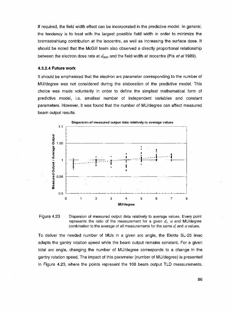
If required, the field width effect can be incorporated in the predictive modal. In general,

the tendency is to treat with the largest possible field width in order to minimize the

bremsstrahlung contribution at the isocentre, as weil as increasing the surface dose. It

should be noted that the McGiII team also observed a directly proportional relationship

between the electron dose rate at dmax and the field width at isocentre (Pla et a/1989).

4.3.2.4 Future work

It should be emphasized that the electron arc parameter corresponding to the number of

MU/degree was not considered du ring the elaboration of the predictive modal. This

choice was made voluntarily in order to define the simplest mathematical form of

predictive model, i.e. smallest number of independent variables and constant

parameters. However, it was found that the number of MU/degree can affect measured

beam output results.

1.1

5 c. 5 o 1.05 CI)

E ~ « 5 c. 5 o

" ~ 0.95 :::1

~ CI)

:E

0.9

Figure 4.23

o

Dispersion of measured output data relatively ta average values

+ + : ...... ' .... ---r .. i ----- ; . +

1 2 3

+ + •

• * +

~ ....... i-------! .... · .. I : , . ; +

*

4

MUfdegree

5 6 7 8

Dispersion of measured output data relatively to average values. Every point represents the ratio of the measurement for a given di, a and MU/degree combination to the average of ail measurements for the same di and avalues.

To deliver the needed number of MUs in a given arc angle, the Elekta SL-25 linac

adapts the gantry rotation speed while the beam output remains constant. For a given

total arc angle, changing the number of MU/degree corresponds to a change in the

gantry rotation speed. The impact of this parameter (number of MU/degree) is presented

in Figure 4.23, where the points represent the 108 beam output TLD measurements.

86

From this figure, it is clear that the number of MU/degree has an impact on the beam

output. This parameter is closely linked to the gantry rotation speed and, therefore, it is

linac related. Since the effect of varying the number of MU/degree was not incorporated

in the predictive model, it will become a source of additional errors when individual TLD

measurements are compared to the predicted values.

Figure 4.24 summarizes the impact of the MU/degree parameter on the overall precision

of the beam output calculation method. The entire set of measured output data, not

average values like in Figure 4.20a, was compared to the corresponding set generated

by the mode!. Despite the spread in the measured data, Figure 4.24 shows that the

calculated beam output data remains a very good approximation for ail measured

electron beam outputs, for ail phantoms and arc angles. Our predictive model remains

clinically acceptable since 89% of the calculated values are within ± 3% of the measured

ones and ail points are within a ± 5% error range (Figure 4.24b).

However, these results clearly demonstrate that the number of MU/degree has to be

considered for further improvement of the mode!. Until full validation of the method is

completed, each calculated number of MUs for a given treatment should be validated

with TLD measurement with phantom of appropriate size and arc conditions before

treatment delivery. Moreover, before clinical implementation, electron arc irradiation

should be performed on different sites of a humanoid phantom. This would allow us to

study every step of the treatment from scanning to delivery and would represent a more

exhaustive verification.

87

Figure 4.24

Comparison between measured and predicted output data

1.2 ,--------------------,

-CIl ... ~ 0.8 ClIS' 111:= .g >. 0.6

-" '5~ a. 0.4 ... ::1 o

0.2

o

a. = 60°

o 0.01 0.02 0.03 0.04

1/djZ [cm·z]

(a)

Histogram of errors between 10 fitted and measured output val ues 9

8

7

~ 6

~ 5

5- 4 ~ 3 iL

2

·4 -2 o Error[%]

(b)

2

108 data points

4

0.05

(a) Comparison between measured data (dots) and curves (solid lines) generated by the predictive model; (b) Histogram of errors: fitted beam output compared to measured beam output for ail individual measurements.

4.4 Clinical implementation

8ased on our results, clinical implementation of the electron arc therapy technique is

possible and it should be facilitated by the following observations regarding our

irradiation conditions:

88

• only small variations of the dmax position;

• a bremsstrahlung contribution always lower than 4.0%;

• a measured therapeutic range R90 between 2 and 3 cm, as required by our

radiation oncologists. Table 4.7 presents a summary of the values obtained in

our treatment configuration after applying a depth scaling correction from acrylic

to water.

Table 4.7 Therapeutic range in acrylic and in water as a function of di, taken from

radial POO measurements in arc irradiations with 0=160° and w=7.3 cm.

di [cm] R;~ry [cm] ~ater [cm]

5.1 2.4 2.7

7.6 2.5 2.8

10.2 2.6 2.9

15.2 2.7 3.0

For clinical cases requiring the R90 of a 10 MeV electron arc beam, the first step is to

establish the total arc angle a and a suitable di from the patient geometry. This part of

the treatment planning can be accomplished based on the CT scan of the patient. A

radiation oncologist has to define the treatment volume first. Then, the volume

information should be used to define the most suitable electron arc in terms of di and a.

Based on the prescribed dose at dmax , the predictive model (equations 3.10 to 3.13) can

be used to calculate the corresponding beam output. At this point, the MU calculation

becomes straightforward, using equation 3.9. Of course, tertiary collimation is necessary

and an appropriate cast has to be built for each patient.

To expand the technique to treat different sites or to cover a wider range of clinical

cases, it would be useful to further investigate certain parameters, such as field width

and energy. According to physicians, increasing the surface dose would be useful to

treat many of the cases that require electron arc therapy. To attain this goal, larger field

sizes would be useful. Oosimetric measurements like the ones performed in this study

89

should also be carried out with lower nominal energies su ch as 6 and 8 MeV. Finally,

extending the study to larger arc angles would be clinically relevant.

90

CHAPTER 5 - CONCLUSION

ln order to characterize the behaviour of electron arc fields, thermoluminescent

dosimeters and film were used in arc irradiation measurements. TLD and film

measurements were compared to measurements performed with an ionization cham ber

in fixed fields. It was shown that TLDs are reliable at ail measurement depths, whereas

films in a parallel orientation are not reliable in the build-up region and that they

overestimate the dose at depths greater than 4 cm. For a 10 MeV nominal energy beam,

this corresponds to the electron practical range region. TLDs were then used to perform

dosimetric measurements including radial PDDs and electron arc beam output at dmax on

the central axis. Films were used to find the positions of dmax for different phantom sizes

and to obtain relative 2D dose distributions in two dimensions, Le. isodose maps for arc

irradiations. At depths greater than 4 cm, 2D isodose maps need to be corrected. This

can be done by referring to TLD measurements. It was observed that overestimation of

dose by films around the electron practical range was greater in arc irradiations than in

fixed fields.

Measurement of radial PDDs along the central axis of cylindrical acrylic phantoms were

performed with a 1 ° MeV nominal energy electron arc beam produced by an Elekta SL-

25 linear accelerator and a dedicated arc applicator. Measurements were performed for

combinations of the following parameters: di values of 5.1, 7.6, 10.2 and 15.2 cm, a

values of 60,90, 120 and 1600 and w values of 3.7,7.3 and 9.8 cm. The influence of

these three parameters was th en studied.

First, the influence of the phantom radius on the PDD and on the dose at dmax was

observed. A change in the phantom radius of curvature (or isocentre depth), di, does not

significantly influence the shape of radial PDDs for the radii values used in this study,

except for a slight shift of the position of dmax to greater depths when the radius

increases. A small increase in the surface dose is also observed when increasing the

phantom diameter. However, the beam output at dmax is larger for phantoms with smaller

radiL

91

Second, the impact of the total arc angle a was studied. Concerning the dose at dmax, an

increase in the angle increases the dose, up to a certain limit angle, after which

additional beams do not contribute significantly to the dose at dmax on the central axis.

For small radii of curvature, dmax receives contributions from ail beams which form the

complete arc, even for large a values. For larger radii of curvature, beams constituting

the entire arc contribute to the dose at dmax only up to a limit avalue, Œ!imit. When beams

are delivered at an angle greater than alimit, no significant dose is added at dmax• This

limit angle is different for every radius of curvature, increasing when the radius gets

sm aller.

The field width at isocentre, w, was shown to have an important influence on radial

PDDs and on the beam output. Increasing w leads to a greater surface dose and to a

shift of dmax towards shallower depths. However, these effects are noticeable only for the

smaller di values in our experiment (smaller than 8 cm).

The influence of field width on the bremsstrahlung contribution to the isocentre was also

studied. It was shown to have a noticeable effect on the bremsstrahlung level in electron

arc irradiations. For small field sizes, on the order of 4 cm, the bremsstrahlung

contribution reaches 8% of the maximum dose in the worst case, whereas it remains

smaller than 4% for ail larger field sizes. As for the output at dmax, an increase in field

size increases the output.

A predictive model was developed, relating the beam output to the phantom size and the

arc angle for a 10 MeV nominal energy electron beam. The model is able to predict the

average measured output data within 3% of the measured values. This was

corroborated by two verification measurements using an intermediate size phantom.

Before clinical use, electron arc irradiation should be performed on a humanoid

phantom. It would allow us to study every step of the treatment, from scanning to

delivery.

As future work, dosimetric measurements with other energies and field sizes should be

carried out, mainly to be able to cover a wider range of clinical cases. To achieve this

goal, characterization of another type of film, such as EOR (Extended Dose Range)

92

radiographie film could be useful for treatment verification. These films could be more

suitable for measurement of higher doses since they have a wider linearity range than

XV films, making them suitable for simultaneous measurements with TLDs.

Also, casts for tertiary collimation on or close to the patient must be built. These casts

must shield radiation efficiently while remaining as comfortable as possible for the

patient. It was shown that a 9 mm thickness of lead meets the shielding requirement.

ln addition, the predictive model for MU calculation should be improved by taking into

account the effect of the field width and the number of MUs per degree.

Finally, a quality assurance (QA) program also needs to be developed for electron arc

therapy, addressing both dosimetric and technical aspects. The dosimetric QA could be

based on what is done for IMRT treatments, which consists of delivery of the treatment

plan to a phantom. For the technical aspect, it should be noted that electron arc therapy,

when delivered dynamically, requires a very reliable linear accelerator. For example,

constancy of the gantry rotation speed should be checked regularly.

93

REFERENCES ALMOND, P.R. et a/ (1999). "AAPM's TG-51 protocol for clinical reference dosimetry of

high-energy photon and electron beams". Med. Phys. 26 (9).1847-1870.

ANDREO, P., SEUNTJENS, J.P., PODGORSAK, E.B. (2003). Review of Radiation

On c%gy Physics: a Handbook for Teachers and Students. E.B. Podgorsak editor.

International Atomic Energy Agency. Vienna, Austria. P. 249-292.

BLAIS, N. (1990). Modified Fermi-Eyges e/ectron scattering in tissue equiva/ent media.

282p. PhD Thesis in Physics, McGili University. Montreal, Canada.

BURNS, D.T., DING, G.X., ROGERS, D.W.O. (1996). "Rso as a beam quality specifier

for selecting stopping-power ratios and reference depths for electron dosimetry". Med.

Phys. 23 (3),383-388.

CAMERON, J.R., SUNTHARALINGAM, N., KENNEY, G.N. (1968). Thermo/uminescent

dosimetry. University of Wisconsin Press, Wisconsin, U.S.A .. 232 pages.

CHILDRESS, N.L., ROSEN, 1.1. (2004). "Effect of processing time delay on the dose

response of Kodak EDR2 film". Med. Phys. 31 (8).2284-2288.

DUTREIX, J., DUTREIX, A. (1969). "Film dosimetry of high-energy electrons". Ann. NY

Acad. Sci. 161, 33-43.

EL-KHATIB, E., ANTOLAK, J, SCRIMGER, J. (1992). "Radiation dose distributions for

electron arc therapy using electrons of 6-20 MeV". Phys. Med. Bio/., Vol. 37, No 6.1375-

1384.

KHAN, F.M. (2003). The Physics of Radiation Therapy. Third edition, Lippincott William

& Wilkins, Philadelphia, U.S.A. 560 pages.

KHAN, F.M., FULLERTON, G.D., LEE, J.M.F., MOORE, V.C., LEVITT, S.H. (1977).

"Physical Aspects of Electron-Beam Arc Therapy". Radi%gy 124.497-500.

94

KLEVENHAGEN, S.C. (1985). Physics of Electron Beam Therapy. Adam Hilger Ltd,

Bristol, England. 204 pages.

LEAVITT, 0.0., PEACOCK, L.M., GIBBS Jr, F.A., STEWART, J.R. (1985). "Electron arc

therapy: physical measurement and treatment planning techniques". Int. J. Radiation

Oncology Biol. Phys., Vol. 11.987-999.

LEAVITT, 0.0., STEWART, J.R., MOELLER, J.H., LEE, W.L., TAKACH Jr, G.A. (1989).

"Electron arc therapy: design, implementation and evaluation of a dynamic multi-vane

collimator system". Int. J. Radiation Oncology Biol. Phys., Vol. 17. 1089-1094.

McKEEVER, S.W.S., MOSCOVITCH, M., TOWNSEND, P.O. (1995).

Thermoluminescence Dosimetry Materials: Properties and Uses. Nuclear Technology

Publishing, England. 204 pages.

McNEELY, L.K., JACOBSON, G.M., LEAVITT, 0.0., STEWART, J.R. (1988). "Electron

arc therapy: chest wall irradiation of breast cancer patients". Int. J. Radiation Oncology

Biol. Phys., Vol. 14. 1287-1294.

PHILIPS MEDICAL SYSTEMS. Patient Support System & Accessories Manual.

Operator's Manuel, Document No. 4522 984 11271 764.

PLA, M., PLA, C., PODGORSAK, E.B. (1988). "The influence of beam parameters on

percentage depth dose in electron arc therapy". Med. Phys. 15 (1). 49-55.

PLA, M., PODGORSAK, E.B., PLA, C. (1989). "Electron dose rate and photon

contamination in electron arc therapy". Med. Phys. 16 (5).692-697.

PLA, M., PODGORSAK, E.B., PLA, C., FREEMAN, C.R. (1993). "Determination of

secondary collimator shape in electron arc therapy". Phys. Med. Biol. 38. 999-1006.

ROBAR, V., ZANKOWSKI, C., OLIVARES PLA, M., PODGORSAK, E.B. (1996).

"Thermoluminescent dosimetry in electron beams: Energy dependence". Med. Phys.23

(5). 667-673.

95

RUEGSEGGER, D.R., LERUDE, S.D., LYLE, D. (1979). "Electron-beam arc therapy

using a high energy betatron". Radiology 133. 483-489.

SHANI, G. (1991). Radiation dosimetry Instrumentation and Methods. CRC Press.

Florida, U.S.A 255 pages.

STRYDOM, W., PARKER, W., OLIVARES, M. (2003). Review of Radiation Oncology

Physics: a Handbook for Teachers and Students. E.S. Podgorsak editor. International

Atomic Energy Agency. Vienna, Austria. P. 225-248.

THWAITES, D.I., DUSAUTOY, AR., JORDAN, T., McEWEN, M.R., NISSET, A,

NAHUM, A.E., PITCHFORD, W.G. (2003). "The IPEM code of practice for electron

dosimetry for radiotherapy beams of initial energy from 4 to 25 MeV based on an

absorbed dose to water calibration". Phys. Med. Biol. 48. 2929-2970.

ZHU, X.R., YOO, S., JURSINIC, P.A, GRIMM, D.F., LOPEZ, F., ROWND, J.J., GILLlN,

M.T. (2003). "Characteristics of sensitometrie curves of radiographie films". Med. Phys.

30 (5). 912-919.

96

5L-25 - McGill Universitydigitool.library.mcgill.ca/thesisfile97944.pdf · ELECTRON ARC THERAPY...

Documents

Transcript of 5L-25 - McGill Universitydigitool.library.mcgill.ca/thesisfile97944.pdf · ELECTRON ARC THERAPY...