5G Radio Measurement Analysis - DiVA...

FACULTY OF ENGINEERING AND SUSTAINABLE DEVELOPMENT .

5G Radio Measurement Analysis

Yves Teganya

June 2016

Master’s Thesis in Electronics

Master’s Program in Electronics/Telecommunications

Examiner: Daniel Rönnow

Supervisors: José Chilo & Magnus Thurfjell

Yves Teganya 5G Radio Measurement Analysis

i

Preface

I would like to thank my supervisors Magnus Thurfjell in Ericsson Research and José Chilo at the

University of Gävle in particular, Ericsson staff in general for the guidance and help in completing this

thesis. I was able to acquire a lot during my short stay in Ericsson.

I would like to thank the academic staff of the Master’s program of Electronics/ Telecommunications

at the University of Gävle and the Swedish Institute for having provided the financial support up to the

completion of the program.

At last, I cordially thank my parents and friends for their moral support, encouragement and love

throughout my studies.


ii

Abstract

The wireless smartphone success, applications and services that keep increasing nowadays, raise the

demand to provide high bitrate; there is a need to find solutions for that requirement. 5G is the next

generation networks that will provide data rates beyond 1Gbps. The aim of this master thesis is to

analyze radio measurements gathered with a 5G radio prototype system operating at 15 GHz, which is

one of the 5G frequency candidates. The focus of this thesis is to primarily search for different

expected and unexpected radio propagation behaviors by comparing measurement results with existing

models and characteristics of existing lower frequency bands. This has been done by modeling the

blocking objects using MATLAB and mapping the results of the blocking model with the

measurements gathered during the blocking.

From the obtained results, it was found that the model response was moving close to the average of the

measurement for reasonable estimation of the obstacles’ dimensions. The model was found to be

sensitive to the height of the obstacles, especially those near the User Equipment (UE). The knife-edge

diffraction model was verified and results were in close agreement with the measurements. The

outcome of the channel estimate analysis is that the signal penetration varied behind the studied tree,

depending on the density of the foliage. Channel gains for the co-polarized antennas at the

Transmission Point (TP) and the UE were found to be 9 dB higher than channel gains for the cross-

polarized antennas at the TP and the UE. Furthermore, the physical separation between antenna

elements at the UE was observed on the MIMO paths when the average channel estimates during the

road sign blocking were calculated and plotted.


iii

Table of contents

Preface ...................................................................................................................................................... i

Abstract ................................................................................................................................................... ii

Table of contents .................................................................................................................................... iii

List of figures .......................................................................................................................................... v

List of tables .......................................................................................................................................... vii

List of abbreviations ............................................................................................................................. viii

1 Introduction ..................................................................................................................................... 1

1.1 Background ............................................................................................................................. 1

1.1 Problem Statement .................................................................................................................. 2

1.2 Aim and methodology ............................................................................................................. 2

1.3 Thesis outline .......................................................................................................................... 2

2 Theory ............................................................................................................................................. 3

2.1 Radio Propagation models ....................................................................................................... 3

2.2 Blocking model ....................................................................................................................... 6

2.3 Knife-edge diffraction model .................................................................................................. 8

2.4 Data rate and beamforming at high frequency bands .............................................................. 9

3 Process, results and discussions .................................................................................................... 10

3.1 Process ................................................................................................................................... 10

3.2 Estimation of the path loss exponent ..................................................................................... 10

3.3 Outdoor blocking Characteristics and model comparison results ......................................... 11

3.3.1 Measurement setup and environment ............................................................................ 11

3.3.2 Road sign ....................................................................................................................... 11

3.3.3 Light pole ...................................................................................................................... 13

3.3.4 Small tree ....................................................................................................................... 15

3.3.5 Big tree .......................................................................................................................... 16

3.3.6 Small truck .................................................................................................................... 17

3.3.7 Van ................................................................................................................................ 18


iv

3.3.8 Garbage truck ................................................................................................................ 20

3.3.9 Sensitivity of the model on the height of the obstacle ................................................... 22

3.3.10 Knife-edge diffraction model response for the van, small truck, and garbage truck ..... 25

3.4 Channel estimate analysis ..................................................................................................... 26

3.4.1 Noisy misaligned and noisy aligned channel estimates ................................................. 26

3.4.2 Channel estimate analysis for the big tree blocking ...................................................... 29

3.4.3 Channel estimate analysis for the garbage truck blocking ............................................ 31

3.5 Impact on polarization and MIMO channel properties ......................................................... 32

4 Conclusions ................................................................................................................................... 35

4.1 Summary of results ................................................................................................................ 35

4.2 Future work ........................................................................................................................... 35

References ............................................................................................................................................. 37

Appendix .............................................................................................................................................. A1


v

List of figures

Figure 1. Classification of fading channels [8]. ...................................................................................... 4

Figure 2. Large-scale and small-scale fading [11]. ................................................................................ 4

Figure 3. Schematic drawing of scattering model [6]. ........................................................................... 6

Figure 4. Shadowing screen model [7]. ................................................................................................... 7

Figure 5. a) Knife-edge diffraction model, b) attenuation as a function of diffraction parameter v [13].8

Figure 6. Difference in path loss as a function of the path loss exponent n in Eq. 1. ........................... 10

Figure 7. a) Transmission Point (TP), b) User Equipment (UE) ........................................................... 11

Figure 8. a) Blocking scenario [21], b) received signal strength for the road sign blocking. ............... 12

Figure 9. Model response mapped with the measurement for the road sign blocking. ......................... 12

Figure 10. a) Blocking scenario [21], b) received signal strength for the light pole blocking. ............. 13

Figure 11. Model response mapped with the measurement for the light pole blocking. ....................... 14

Figure 12. Model response mapped with the measurement for the light pole and the person blocking.

............................................................................................................................................................... 14

Figure 13. a) Blocking scenario [21], b) received signal strength for the small tree blocking. ............ 15

Figure 14. Model response mapped with the measurement for the small tree blocking. ...................... 15

Figure 15. a) Blocking scenario [21], b) received signal strength for the big tree blocking. ............... 16

Figure 16. Model response mapped with the measurement for the big tree blocking. .......................... 17

Figure 17. a) Blocking scenario [21], b) received signal strength for the small truck blocking. ......... 17

Figure 18. Model response mapped with the measurement for the small truck blocking. .................... 18

Figure 19. Blocking scenario: a) van, b) pedestrians ............................................................................ 18

Figure 20. Received signal strength for a blocking combination made of tree, van, and pedestrians. .. 19

Figure 21. Model response mapped with the measurement for the van blocking. ................................ 19

Figure 22. Garbage truck blocking scenario.......................................................................................... 20

Figure 23. Received signal strength for the big garbage truck blocking. .............................................. 20

Figure 24. Truck modelling and position along the street (m). ............................................................. 21

Figure 25. Model response mapped with the measurement for the garbage truck blocking. ................ 22

Figure 26. Garbage truck model response for UE antenna height ranging from 0 to 3 m. ................... 23

Figure 27. Relative power as a function of the UE antenna height for the garbage truck blocking. ..... 23

Figure 28. Big tree model response: a) for the assumed tree height and ±2 % on tree height, b) for UE

antenna height ranging from 0 to 4 m. .................................................................................................. 24

Figure 29. Relative power as a function of the UE antenna height for the big tree blocking. .............. 24

Figure 30. UE test route with position of the road sign, the small tree, the big tree, and the TP [21]. . 27

Figure 31. Misaligned channel estimate. ............................................................................................... 27

Figure 32. Aligned channel estimate. .................................................................................................... 28


vi

Figure 33. a) Propagation scenarios (both LoS), b) PDPs at the 123rd and the 125th seconds. ............ 29

Figure 34. a) Propagation scenarios, b) PDPs at the 123rd, 138th, and 139th seconds. ........................... 29

Figure 35. a) Propagation scenarios, b) PDPs at the 123rd, 148th, and 149th seconds. ........................... 30

Figure 36. Reflections at the 123rd and 148th (or 149th) seconds. ........................................................... 31

Figure 37. a) Some of Ki30 façade structures, b) PDPs at the 20th, 22.45, 22.55, 22.7, 23, and 23.5

seconds. ................................................................................................................................................. 32

Figure 38. Average channel gains of a 2.5-second long LoS scenario. The paths TX1-RX3 and TX3-

RX1 are for the co-polarization. The paths TX2-RX4 and TX4-RX2 are for the cross polarization.... 33

Figure 39. Channel gains during the road sign blocking. ...................................................................... 34

Figure 40. Channel gains during the garbage truck blocking. ............................................................... 34


vii

List of tables

Table 1. Dimensions of the obstacles used in the modeling and the distance to the UE. ...................... 25

Table 2. Comparison of the measurement attenuation and the knife-edge diffraction model response

for the van, the small truck, and the garbage truck. .............................................................................. 25

Table 3. Obstacles’ blocking loss for outdoor to outdoor and outdoor to indoor measurements [20],

[21]. ....................................................................................................................................................... 26

Table 4. Average channel gains in dB of a 2.5-second long LoS scenario for the 4×4 MIMO paths ... 32


viii

List of abbreviations

CDM Code Division Multiplexing

HDR High Dynamic Range

HSPA High Speed Packet Access

IRR Infrared reflecting

LTE Long Term Evolution

LoS Line of Sight

METIS Mobile and wireless communications Enablers for the Twenty-twenty

Information Society

MIMO Multiple Input Multiple Output

OFDM Orthogonal frequency division multiplexing

OLoS Obstructed Line of Sight

PDP Power Delay Profile

TDM Time Division Multiplexing

TP Transmission Point

TX Transmitter

RX Receiver

UE User Equipment

WCDMA Wideband Code Division Multiple Access


1

1 Introduction

This section contains the background, introduces the problem to be solved, and gives the aim of the

thesis with the methodology used in solving the problem. Furthermore, it gives the outline of the rest

of the thesis.

1.1 Background

The area of telecommunications has become very rich; there is continuity in the upgrade of services

and platforms from one generation to another. There has been tremendous development from the first

generation networks (1G) deployed in 1980, which were entirely analog for voice communications, up

to now [1]. Digital modulation schemes such as TDM, CDM were implemented in the second

generation networks (2G). In the third generation networks (3G), there was a high improved

multimedia streaming with the use of HSPA and WCDMA. 3G networks were improved to Evolved

HSPA (HSPA+). LTE is the radio access for 4G networks; it is an OFDM technique that uses up to 20

MHz of bandwidth with multiple antenna transmission structure. The data rate with 4G network goes

beyond 100Mbps [2].

The wireless smartphone success increases the demand to provide high bitrate. Applications and

services that keep increasing nowadays are expected to be available wireless with the same experience

as if provided over fiber (with or greater than 1Gigabit per second of data rate). The wireless bitrate is

limited by physical constraints such as the frequency bandwidth. At frequency bands today used for

LTE and Wi-Fi, it is difficult to find contiguous and suitable frequency regions to expand emerging

accesses into. For 5G radio access there is therefore research on the possibility to use even higher

frequency bands, from 6 GHz all the way up to mm-wavelength at 60 GHz. At higher frequency bands

the radio propagation and its corresponding characteristics are expected to be somewhat different,

which might require different solutions and features.

With 5G networks, bandwidths of several hundreds of MHz are expected, going even beyond 1GHz

[2]. High data rates will be achieved at the expense of the propagation distance [3, 4] due to the small

effective area of the antenna and high path loss. 5G networks will enable broadband experience

everywhere, anytime in crowed areas, public transport, and event platforms. 5G is found to be much

useful in smart vehicles, transport and infrastructure with self-driving and connected cars in order to

avoid traffic jam and accidents. Media everywhere is one of the use cases of 5G where in-home and

mobile TV, ultimate video quality (4K, 8K, HDR) are expected. 5G will be crucial in critical control

of remote devices where robots are operated remotely, remote surgery is possible, and automation of

industries. None can leave behind human interactions through Internet of Things with 5G; this is


2

where one can say that everything will be smart, such as smart houses and many tools and equipment

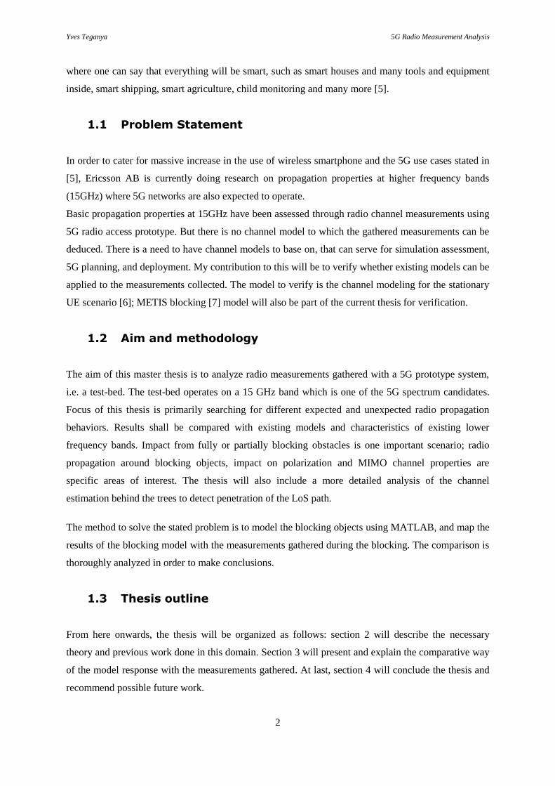
inside, smart shipping, smart agriculture, child monitoring and many more [5].

1.1 Problem Statement

In order to cater for massive increase in the use of wireless smartphone and the 5G use cases stated in

[5], Ericsson AB is currently doing research on propagation properties at higher frequency bands

(15GHz) where 5G networks are also expected to operate.

Basic propagation properties at 15GHz have been assessed through radio channel measurements using

5G radio access prototype. But there is no channel model to which the gathered measurements can be

deduced. There is a need to have channel models to base on, that can serve for simulation assessment,

5G planning, and deployment. My contribution to this will be to verify whether existing models can be

applied to the measurements collected. The model to verify is the channel modeling for the stationary

UE scenario [6]; METIS blocking [7] model will also be part of the current thesis for verification.

1.2 Aim and methodology

The aim of this master thesis is to analyze radio measurements gathered with a 5G prototype system,

i.e. a test-bed. The test-bed operates on a 15 GHz band which is one of the 5G spectrum candidates.

Focus of this thesis is primarily searching for different expected and unexpected radio propagation

behaviors. Results shall be compared with existing models and characteristics of existing lower

frequency bands. Impact from fully or partially blocking obstacles is one important scenario; radio

propagation around blocking objects, impact on polarization and MIMO channel properties are

specific areas of interest. The thesis will also include a more detailed analysis of the channel

estimation behind the trees to detect penetration of the LoS path.

The method to solve the stated problem is to model the blocking objects using MATLAB, and map the

results of the blocking model with the measurements gathered during the blocking. The comparison is

thoroughly analyzed in order to make conclusions.

1.3 Thesis outline

From here onwards, the thesis will be organized as follows: section 2 will describe the necessary

theory and previous work done in this domain. Section 3 will present and explain the comparative way

of the model response with the measurements gathered. At last, section 4 will conclude the thesis and

recommend possible future work.


3

2 Theory

This section discusses the previous work done on some existing propagation models and fading.

Furthermore, it presents the techniques used for the obtainment of high data rates at high frequency

bands.

2.1 Radio Propagation models

The behavior of a communication channel determines the performance of a wireless system. The

wireless channel behaves in a stochastic way (thus making it unpredictable) compared to the wired

channel. High performance and bandwidth efficient communication systems can be achieved if

wireless channels are better understood [8].

In wireless communication systems, radio waves travel in different ways from the transmitter to the

receiver. In addition to propagation in the air, the three main mechanisms in radio propagation are [9],

[10]:

Reflection: where the propagating wave hits an object with dimensions larger compared to the

wavelength. Surface of earth, buildings, cars are examples where reflections can occur.

Diffraction: phenomenon that occurs when there is obstruction in the direct radio path

between the transmitter and the receiver. Diffraction can happen on surfaces with sharp

abnormalities or apertures.

Scattering: occurs when the propagating medium is made of objects smaller than the

wavelength of the radio wave. Objects that can cause scattering are foliage, street signs, and

lamp posts.

These mechanisms make the channel unpredictable. The propagation from the transmitter to the

receiver may occur without any of the three phenomena to happen; in other cases, all or some of them

can happen in different scenarios depending on the environment. As the propagating wave goes

through the different mechanisms, its amplitude reduces, its frequency and phase change (Doppler

effect). This is known as fading. Additive noise, interfering signals are also the causes of the signal

fading [8].

Fading is of two types: large-scale fading and small-scale fading. Large-scale fading is caused by loss

of signal when the receiver is moving over large distances passing through different terrain profiles

such as buildings, intervening pastures, and vegetation. Large-scale fading is the average path loss and

shadowing. On the other hand, when the receiver moves over short distances, there are rapid variations

of signal level due to the additive and subtractive interference of multiple signal paths (multi-paths).

This is known as small-scale fading. In small-scale fading, we have frequency selective fading or flat


4

fading when the coherence bandwidth of the channel is smaller or greater than the bandwidth of the

signal to be transmitted.

Small-scale fading can as well be classified as either fast fading or slow fading depending on whether

the coherence time of the channel is smaller or greater than the symbol period of the transmitted

signal. Fig. 1 shows the classification of fading in radio propagation [8].

Figure 1. Classification of fading channels [8].

Small-scale fading is usually considered to be Rayleigh distributed when no strong LoS component is

present and Ricean distributed if there is such a component. Large-scale fading is usually modelled as

log-normally distributed. Fig. 2 shows the received signal power for large-scale and small-scale fading

as a function of the distance [11].

Figure 2. Large-scale and small-scale fading [11].

In the link budget calculation of a radio channel, the free space path loss FSL (for n=2), is given by

[12]

n

R

TFS

d

P

PL

4 (1)


5

with f

c (2)

where TP - is the transmitted power in W

RP - is the received power in W

d - is the distance between the transmitter and the receiver in m

c - is the speed of light in m/s

f - is the carrier frequency in Hz.

In dB, the free space path loss is given by

)log(20)log(204.32 dfLFS (3)

where the frequency f is in MHz and the distance d is in km.

For the plane earth model, the path loss PEL , in dB is given by [13]

)log(40)log(20 21 dhhLPE (4)

where 1h and 2h are the transmitter and the receiver antenna heights, respectively.

Free space and plane earth path loss models are examples of what is denoted as power law models

with path loss expressed in dB as [13]

KdnL log10 (5)

with knK log10 (6)

where n - is the path loss exponent

k- is a constant depending on the propagation scenario

K-is the clutter factor.

Another example of power law model is the Delisle-Egli model described in [14].

While dealing with a more realistic channel, the log-normal shadowing model is used. If G is a

Gaussian random variable with zero mean and standard deviation , reference distance 0d , and path

loss exponent n; the path loss )(dL , at distance d from the transmitter is given by [15]

Gd

dnLL dd

0

)()( log100

(7)

where )( 0dL is the path loss at the reference known distance 0d .

Okomura [16] made comprehensible empirical path loss models for a range of antenna heights,

frequency range and coverage areas. Hata [17] changed Okumura’s results and obtained parametric

formulae.


6

2.2 Blocking model

Using Fourier series and according to fig. 3, the expression for shadowing shF , is given by [6]

N

Nk

ik

ksh efF . (8)

where

ki

k

kf

sh

k .2

exp..

).sin(

(9)

For plane waves,

2

1

5R (10)

Figure 3. Schematic drawing of scattering model [6].

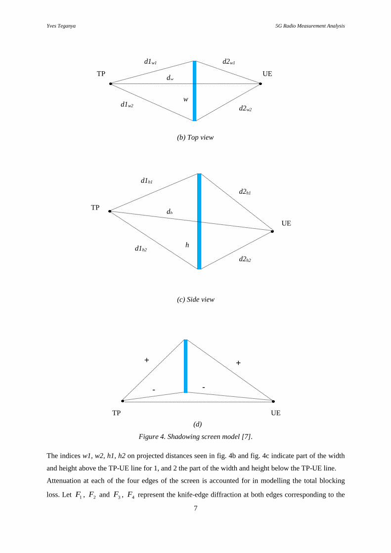
For simplicity in the modeling, the obstacle between the TP and the UE is estimated as a rectangular

screen (see fig. 4a). The screen is assumed to be vertical and moves along a vertical axis through its

center whenever either node (TP or UE) is moving so that the screen is always perpendicular to the

line connecting the TP and the UE [7]. Top and side views are seen in fig. 4b and fig. 4c, respectively.

Fig. 4a

TP UE


7

(b) Top view

(c) Side view

(d)

Figure 4. Shadowing screen model [7].

The indices w1, w2, h1, h2 on projected distances seen in fig. 4b and fig. 4c indicate part of the width

and height above the TP-UE line for 1, and 2 the part of the width and height below the TP-UE line.

Attenuation at each of the four edges of the screen is accounted for in modelling the total blocking

loss. Let 1F , 2F and 3F , 4F represent the knife-edge diffraction at both edges corresponding to the

TP UE

TP

UE

TP UE

+

+

-

-

d1w1 d2w1

d1w2 d2w2

dw

w

d1h1

d2h1

d1h2

d2h2

dh

h


8

width w and the height h, respectively. The overall blocking (shadowing) loss of the screen is modeled

as

)))((1(log20)( 432110 FFFFdBL (11)

For one edge, the shadowing is calculated using the knife-edge diffraction as [7]

ddd

F

21

1

2tan

(12)

where 1d - is the projected distance between the TP and the edges of the screen ( 11wd , 21wd , 11hd ,

and 21hd on fig. 4b and 4c)

2d - is the projected distance between the UE and the edges of the screen ( 12wd , 22wd , 12hd ,

and 22hd on fig. 4b and c)

d - is the projected distance between the TP and the UE

- is the wavelength.

The plus sign in Eq. 12 stands for the shadow zone. When the TP and the UE are in OLoS, the plus

sign applies to all edges of the screen. In the LoS scenario, the plus sign is applied to the edge farther

from the link (considered to be in shadow zone) and the minus sign to the edge closer to the link (see

fig. 4d) [7].

2.3 Knife-edge diffraction model

The knife-edge diffraction model seen in fig. 5 is used to approximate the additional attenuation

introduced by an obstacle (in green) due to diffraction. The received signal depends on the height h.

(a) (b)

Figure 5. a) Knife-edge diffraction model, b) attenuation as a function of diffraction parameter v [13].


9

Assuming h < < 1d , 2d and h >> , the diffraction parameter v is given by [13]

21

21 )(2

dd

ddhv

(13)

The parameter v obtained using Eq. 13 for a given obstruction allows, using the graph in fig. 5b to

obtain the corresponding attenuation.

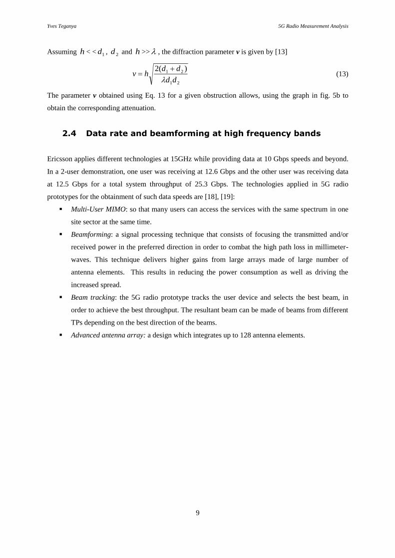
2.4 Data rate and beamforming at high frequency bands

Ericsson applies different technologies at 15GHz while providing data at 10 Gbps speeds and beyond.

In a 2-user demonstration, one user was receiving at 12.6 Gbps and the other user was receiving data

at 12.5 Gbps for a total system throughput of 25.3 Gbps. The technologies applied in 5G radio

prototypes for the obtainment of such data speeds are [18], [19]:

Multi-User MIMO: so that many users can access the services with the same spectrum in one

site sector at the same time.

Beamforming: a signal processing technique that consists of focusing the transmitted and/or

received power in the preferred direction in order to combat the high path loss in millimeter-

waves. This technique delivers higher gains from large arrays made of large number of

antenna elements. This results in reducing the power consumption as well as driving the

increased spread.

Beam tracking: the 5G radio prototype tracks the user device and selects the best beam, in

order to achieve the best throughput. The resultant beam can be made of beams from different

TPs depending on the best direction of the beams.

Advanced antenna array: a design which integrates up to 128 antenna elements.


10

3 Process, results and discussions

This section explains the process, presents and discusses the results of each blocking object.

Furthermore, it contains the channel estimate analysis through the power delay profiles (PDPs). The

impact of polarization and MIMO channel properties are also addressed herein.

3.1 Process

Dimensions of the blocking objects as well as the distance to the TP and the UE have been used in

Eqs. 2, 11 and 12 to produce the model response in MATLAB. The produced model has then been

mapped with the gathered logged measurement for comparison and analysis. For some objects,

dimensions were slightly changed to see and better understand the model verification. Before delving

into the measurements and blocking model, the estimation of the path loss exponent has been done.

3.2 Estimation of the path loss exponent

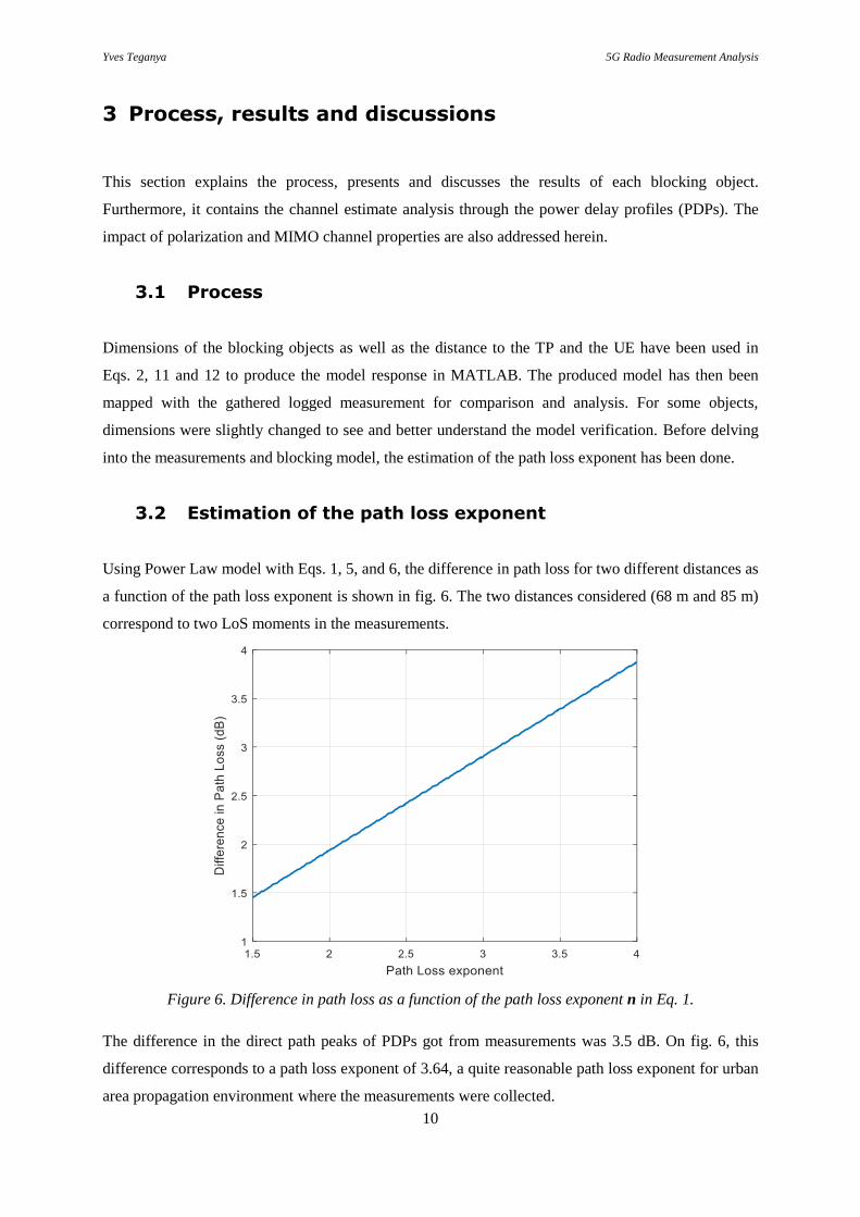
Using Power Law model with Eqs. 1, 5, and 6, the difference in path loss for two different distances as

a function of the path loss exponent is shown in fig. 6. The two distances considered (68 m and 85 m)

correspond to two LoS moments in the measurements.

Figure 6. Difference in path loss as a function of the path loss exponent n in Eq. 1.

The difference in the direct path peaks of PDPs got from measurements was 3.5 dB. On fig. 6, this

difference corresponds to a path loss exponent of 3.64, a quite reasonable path loss exponent for urban

area propagation environment where the measurements were collected.


11

3.3 Outdoor blocking Characteristics and model comparison

results

3.3.1 Measurement setup and environment

The measurement equipment is made of a TP mounted at an office building at a height of 12 m. The

UE is installed on an electric scooter and moves approximately at a speed of 0.5 m/s with its antenna

mounted at 1.5 m above the ground. The TP and the UE are seen in fig. 7. The measurements were

gathered in Kista, an urban area in Stockholm.

(a) (b)

Figure 7. a) Transmission Point (TP), b) User Equipment (UE)

A 100 MHz bandwidth carrier at 14.9 GHz is used. When two carriers are used, the total transmitted

power is 1 W. The gain of each antenna element is 15 dBi with half power beamwidths being 90º and

8.6 º for azimuth and elevation, respectively. The UE antenna is considered to be omnidirectional with

a gain of -3 dBi and 4 dB feeder loss. We have an array with two dual-polarized antenna elements at

the TP and the UE; thus, allowing 4×4 MIMO spatial multiplexing per carrier. The multiplexing

scheme of the radio channel is OFDM and the noise floor is considered to be -75 dBm; below this

power level, the synchronization between the TP and the UE fails [20]. Blocking object cases

considered are road sign, light pole, small tree, big tree, small truck, van, and garbage truck [21].

The carrier 1 was used. In the received signal variations and the mapped measurements with the model

response (in figures of subsection 3.3.2 to subsection 3.3.9), a new sample was taken after an interval

of 5 milliseconds, yielding to 200 samples in a second [20].

3.3.2 Road sign

The blocking is illustrated in fig. 8a. In fig. 8b, the received power as the UE moves and the road sign

obstructs the TP –UE link can be seen.

In fig. 8b, the red box frames the received signal variations when the road sign blocks the LoS. The

maximum signal attenuation is around 5 dB. The two peaks before and after the signal fade indicate

the scattering effects when passing the road sign [21].


12

(a) (b)

Figure 8. a) Blocking scenario [21], b) received signal strength for the road sign blocking.

The attenuation components accounting for the knife-edge diffraction corresponding to the height of

the road sign 3F and 4F in the equation

)))((1(log20)( 432110 FFFFdBL

with

ddd

F

21

1

4/3/2/1

2tan

are approximately equal to 0.5 each. Adding these two components leads roughly to 1. Besides, there

is no lower edge of the screen as the road sign is planted into the ground. For simplicity, the road sign

was considered to be infinitely high. The attenuation of the incoming signal caused by the road sign is

mainly due to the road sign side edges (diameter). The model response of the road sign mapped with

the measurement is seen in fig. 9.

Figure 9. Model response mapped with the measurement for the road sign blocking.


13

From fig. 9, the Ø60 mm road sign gave the response seen in green. There was around 1 m between

the road sign and the UE, the distance between the TP and the UE was estimated to 68 m. The model

response follows the mean of measurement, but a difference of 2 dB at the maximum blocking

moment is observed. The response seen in red corresponds to a Ø100 mm road sign. The increment in

the road sign radius brings the model to fit better in the measurement with only a difference of 0.5 dB

at the maximum obstruction moment.

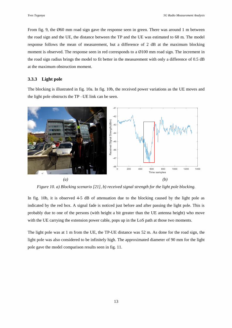
3.3.3 Light pole

The blocking is illustrated in fig. 10a. In fig. 10b, the received power variations as the UE moves and

the light pole obstructs the TP –UE link can be seen.

(a) (b)

Figure 10. a) Blocking scenario [21], b) received signal strength for the light pole blocking.

In fig. 10b, it is observed 4-5 dB of attenuation due to the blocking caused by the light pole as

indicated by the red box. A signal fade is noticed just before and after passing the light pole. This is

probably due to one of the persons (with height a bit greater than the UE antenna height) who move

with the UE carrying the extension power cable, pops up in the LoS path at those two moments.

The light pole was at 1 m from the UE, the TP-UE distance was 52 m. As done for the road sign, the

light pole was also considered to be infinitely high. The approximated diameter of 90 mm for the light

pole gave the model comparison results seen in fig. 11.


14

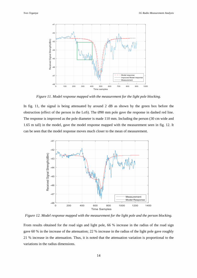
Figure 11. Model response mapped with the measurement for the light pole blocking.

In fig. 11, the signal is being attenuated by around 2 dB as shown by the green box before the

obstruction (effect of the person in the LoS). The Ø90 mm pole gave the response in dashed red line.

The response is improved as the pole diameter is made 110 mm. Including the person (30 cm wide and

1.65 m tall) in the model, gave the model response mapped with the measurement seen in fig. 12. It

can be seen that the model response moves much closer to the mean of measurement.

Figure 12. Model response mapped with the measurement for the light pole and the person blocking.

From results obtained for the road sign and light pole, 66 % increase in the radius of the road sign

gave 60 % in the increase of the attenuation; 22 % increase in the radius of the light pole gave roughly

21 % increase in the attenuation. Thus, it is noted that the attenuation variation is proportional to the

variations in the radius dimensions.


15

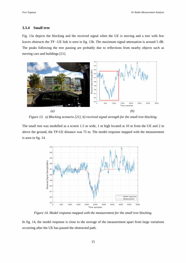
3.3.4 Small tree

Fig. 13a depicts the blocking and the received signal when the UE is moving and a tree with few

leaves obstructs the TP –UE link is seen in fig. 13b. The maximum signal attenuation is around 5 dB.

The peaks following the tree passing are probably due to reflections from nearby objects such as

moving cars and buildings [21].

(a) (b)

Figure 13. a) Blocking scenario [21], b) received signal strength for the small tree blocking.

The small tree was modelled as a screen 1.5 m wide, 1 m high located at 10 m from the UE and 2 m

above the ground, the TP-UE distance was 75 m. The model response mapped with the measurement

is seen in fig. 14.

Figure 14. Model response mapped with the measurement for the small tree blocking.

In fig. 14, the model response is close to the average of the measurement apart from large variations

occurring after the UE has passed the obstructed path.


16

3.3.5 Big tree

The blocking and the received signal variations when the UE is moving and a tree with more leaves

obstructs the TP –UE link are seen in fig. 15a and 15b, respectively.

(a) (b)

Figure 15. a) Blocking scenario [21], b) received signal strength for the big tree blocking.

In fig. 15b, the red boxes indicate the rapid variations due the scattering objects of the obstacle

(leaves). The average attenuation compared to the free space received power is around 7 dB. In the

same figure, the dashed green line acting as line of symmetry indicates the point of return (the point

where the UE takes the reverse direction and returns back to its starting point).

The length and the height of the tree (modelled as a screen) were approximated to 7.8 m and 4 m,

respectively. The TP-UE distance was 95 m and the tree was at a distance of 35 m from the UE and 2

m above the ground. The tree stem was omitted for simplicity in the modelling as it was much below

TP-UE link. The model comparison results are seen in fig. 16. Despite its “see-through” properties,

the tree fits the model. The model response simulation ends at the turning point of the UE, a similar

response would have been obtained if the UE had continued in the same direction and move out of the

tree obstruction; it can also be seen that the response follows the mean of the measurement.


17

Figure 16. Model response mapped with the measurement for the big tree blocking.

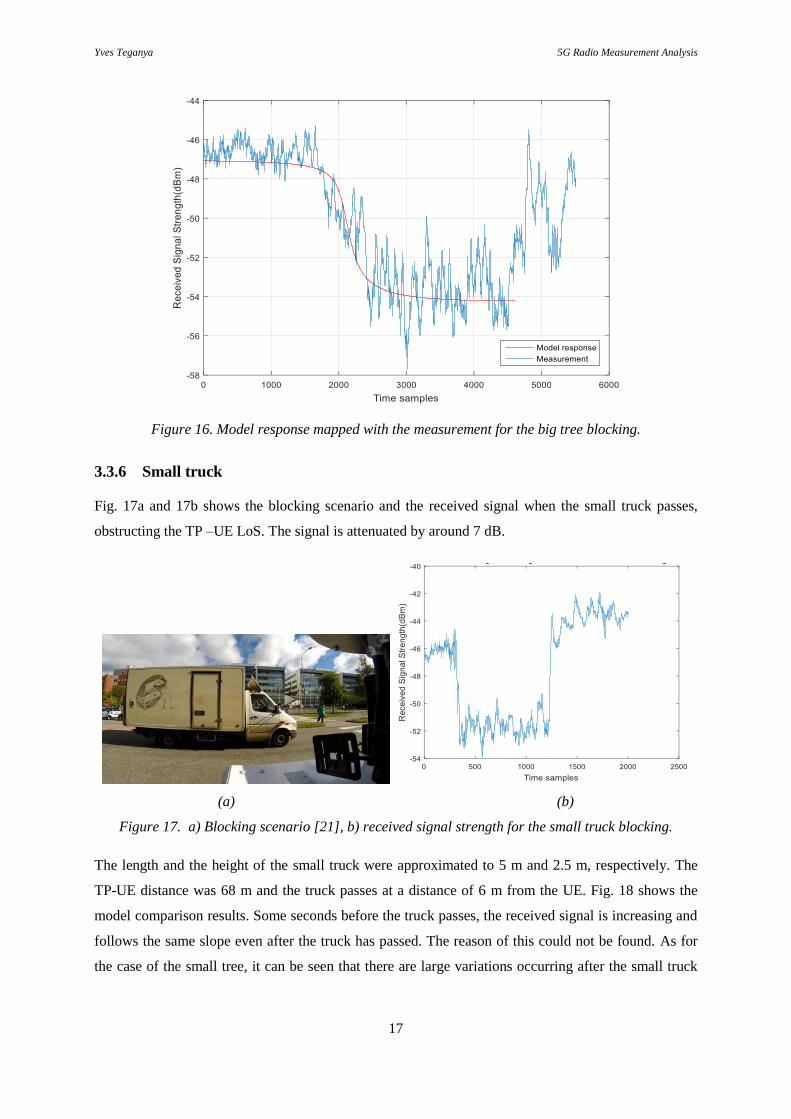
3.3.6 Small truck

Fig. 17a and 17b shows the blocking scenario and the received signal when the small truck passes,

obstructing the TP –UE LoS. The signal is attenuated by around 7 dB.

(a) (b)

Figure 17. a) Blocking scenario [21], b) received signal strength for the small truck blocking.

The length and the height of the small truck were approximated to 5 m and 2.5 m, respectively. The

TP-UE distance was 68 m and the truck passes at a distance of 6 m from the UE. Fig. 18 shows the

model comparison results. Some seconds before the truck passes, the received signal is increasing and

follows the same slope even after the truck has passed. The reason of this could not be found. As for

the case of the small tree, it can be seen that there are large variations occurring after the small truck


18

has passed and the model response deviates from the measurement. Reasons might be reflections from

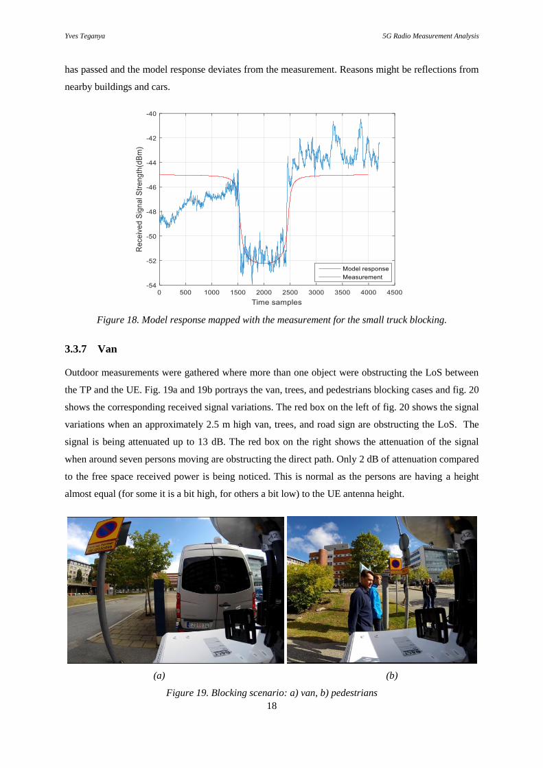
nearby buildings and cars.

Figure 18. Model response mapped with the measurement for the small truck blocking.

3.3.7 Van

Outdoor measurements were gathered where more than one object were obstructing the LoS between

the TP and the UE. Fig. 19a and 19b portrays the van, trees, and pedestrians blocking cases and fig. 20

shows the corresponding received signal variations. The red box on the left of fig. 20 shows the signal

variations when an approximately 2.5 m high van, trees, and road sign are obstructing the LoS. The

signal is being attenuated up to 13 dB. The red box on the right shows the attenuation of the signal

when around seven persons moving are obstructing the direct path. Only 2 dB of attenuation compared

to the free space received power is being noticed. This is normal as the persons are having a height

almost equal (for some it is a bit high, for others a bit low) to the UE antenna height.

(a) (b)

Figure 19. Blocking scenario: a) van, b) pedestrians


19

Figure 20. Received signal strength for a blocking combination made of tree, van, and pedestrians.

The dimensions of the van used are 3 m and 2.5 m for width and height, respectively. The estimated

width exceeds the physical van width because of the parking condition and TP location (see fig. 19a).

The van was assumed to be parked at 4.5 m from the UE route with the TP-UE distance being 60 m.

Initial and improved model responses in dashed and solid red lines are seen in fig. 21.

Figure 21. Model response mapped with the measurement for the van blocking.

Blocking combination made of a van,

trees, and road sign

Pedestrians in the LoS


20

In fig. 21, 2 seconds (400 measurement samples) after entering the van shadow zone, the measurement

deviates from the model response and the signal is increased by around 3 dB, but still in the

obstruction. This is due to the change in the obstruction scenario, the UE moves from the rear part of

the van to the lateral part of it where the signal is better received due to less effect caused by

diffraction. Decreasing the “effective” obstruction width of the van by 10 %, gave the improved

model response shown in the solid red line on the same figure fitting better with the measurement.

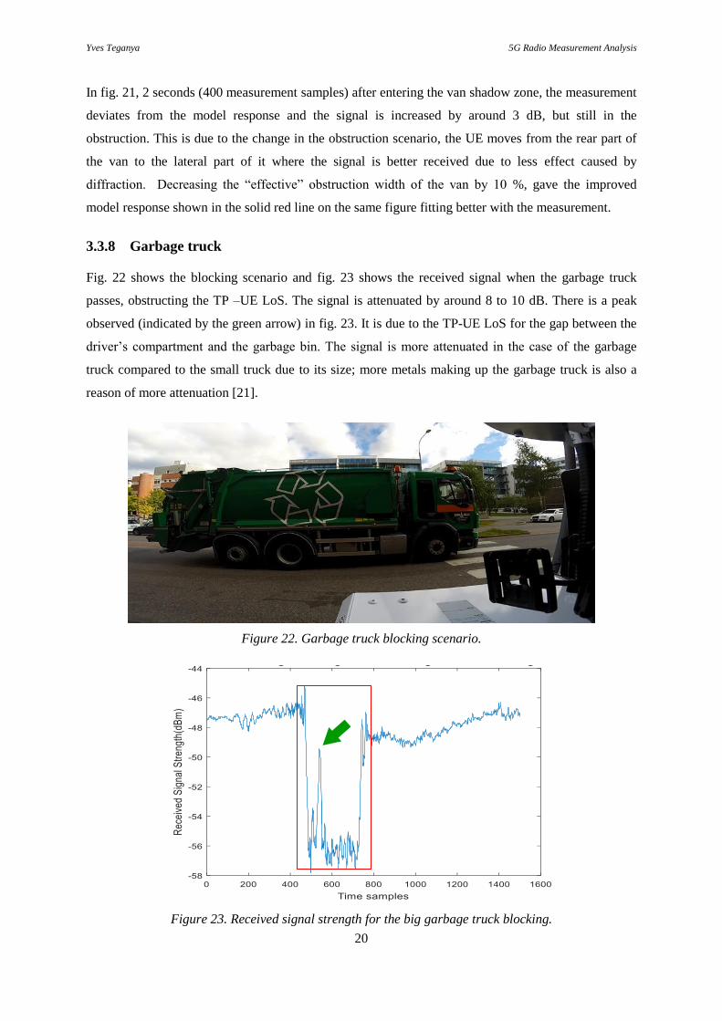
3.3.8 Garbage truck

Fig. 22 shows the blocking scenario and fig. 23 shows the received signal when the garbage truck

passes, obstructing the TP –UE LoS. The signal is attenuated by around 8 to 10 dB. There is a peak

observed (indicated by the green arrow) in fig. 23. It is due to the TP-UE LoS for the gap between the

driver’s compartment and the garbage bin. The signal is more attenuated in the case of the garbage

truck compared to the small truck due to its size; more metals making up the garbage truck is also a

reason of more attenuation [21].

Figure 22. Garbage truck blocking scenario.

Figure 23. Received signal strength for the big garbage truck blocking.


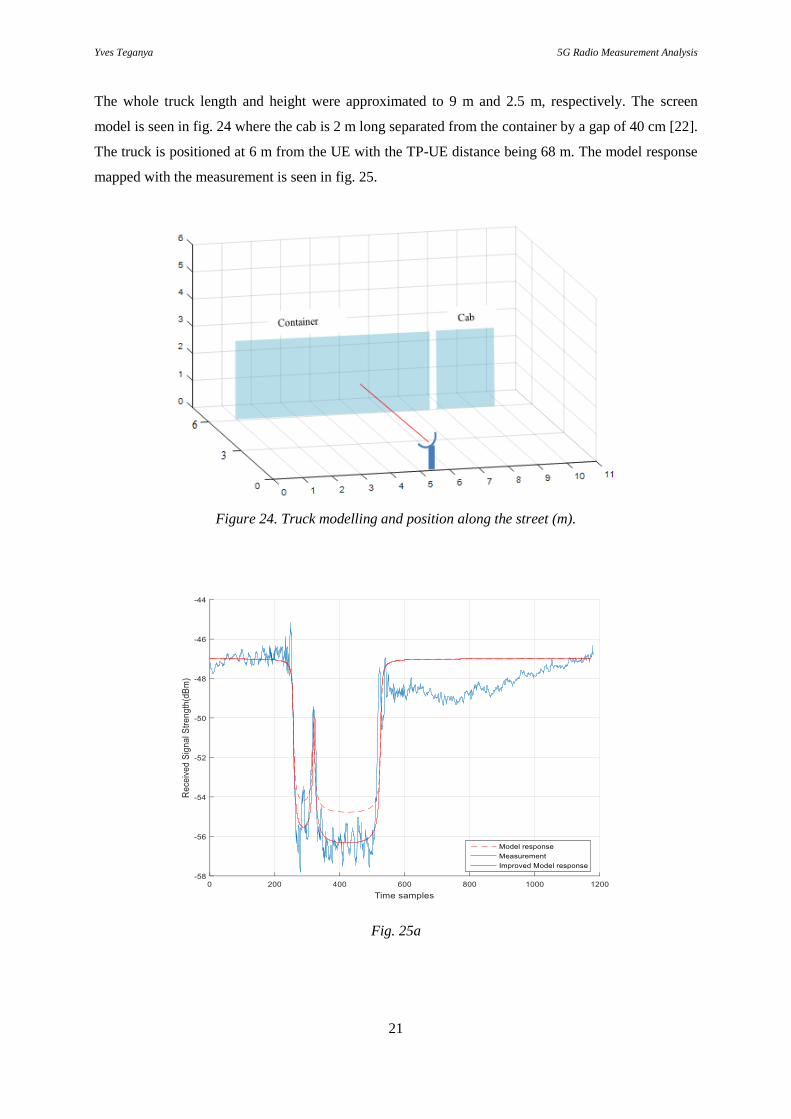
21

The whole truck length and height were approximated to 9 m and 2.5 m, respectively. The screen

model is seen in fig. 24 where the cab is 2 m long separated from the container by a gap of 40 cm [22].

The truck is positioned at 6 m from the UE with the TP-UE distance being 68 m. The model response

mapped with the measurement is seen in fig. 25.

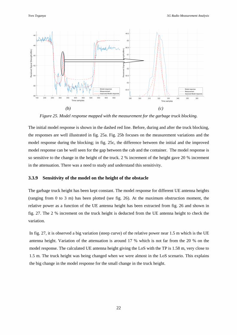
Figure 24. Truck modelling and position along the street (m).

Fig. 25a


22

(b) (c)

Figure 25. Model response mapped with the measurement for the garbage truck blocking.

The initial model response is shown in the dashed red line. Before, during and after the truck blocking,

the responses are well illustrated in fig. 25a. Fig. 25b focuses on the measurement variations and the

model response during the blocking; in fig. 25c, the difference between the initial and the improved

model response can be well seen for the gap between the cab and the container. The model response is

so sensitive to the change in the height of the truck. 2 % increment of the height gave 20 % increment

in the attenuation. There was a need to study and understand this sensitivity.

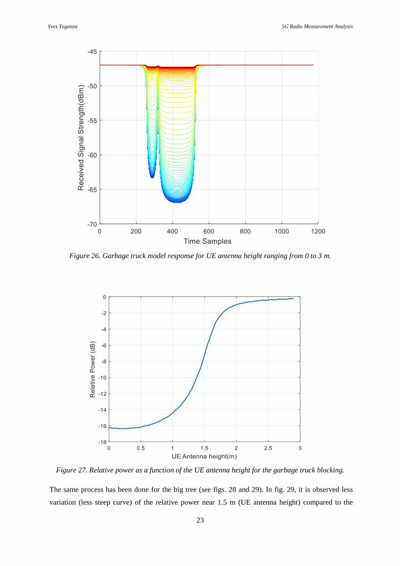
3.3.9 Sensitivity of the model on the height of the obstacle

The garbage truck height has been kept constant. The model response for different UE antenna heights

(ranging from 0 to 3 m) has been plotted (see fig. 26). At the maximum obstruction moment, the

relative power as a function of the UE antenna height has been extracted from fig. 26 and shown in

fig. 27. The 2 % increment on the truck height is deducted from the UE antenna height to check the

variation.

In fig. 27, it is observed a big variation (steep curve) of the relative power near 1.5 m which is the UE

antenna height. Variation of the attenuation is around 17 % which is not far from the 20 % on the

model response. The calculated UE antenna height giving the LoS with the TP is 1.58 m, very close to

1.5 m. The truck height was being changed when we were almost in the LoS scenario. This explains

the big change in the model response for the small change in the truck height.


23

Figure 26. Garbage truck model response for UE antenna height ranging from 0 to 3 m.

Figure 27. Relative power as a function of the UE antenna height for the garbage truck blocking.

The same process has been done for the big tree (see figs. 28 and 29). In fig. 29, it is observed less

variation (less steep curve) of the relative power near 1.5 m (UE antenna height) compared to the


24

garbage truck case. The main reason is that the tree is far from the UE compared to the truck, which

passes closer to the UE. The variation of the attenuation is around 9 % while we have 14 % on the

model response.

(a) (b)

Figure 28. Big tree model response: a) for the assumed tree height and ±2 % on tree height, b) for UE

antenna height ranging from 0 to 4 m.

Figure 29. Relative power as a function of the UE antenna height for the big tree blocking.

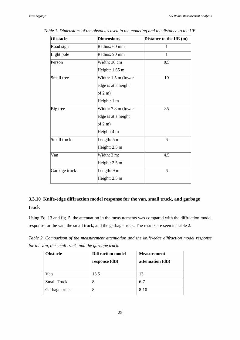
Table 1 summarizes the dimensions of the obstacles used in the modeling and their respective

distances to the UE.


25

Table 1. Dimensions of the obstacles used in the modeling and the distance to the UE.

Obstacle Dimensions Distance to the UE (m)

Road sign Radius: 60 mm 1

Light pole Radius: 90 mm 1

Person Width: 30 cm

Height: 1.65 m

0.5

Small tree Width: 1.5 m (lower

edge is at a height

of 2 m)

Height: 1 m

10

Big tree Width: 7.8 m (lower

edge is at a height

of 2 m)

Height: 4 m

35

Small truck Length: 5 m

Height: 2.5 m

6

Van Width: 3 m:

Height: 2.5 m

4.5

Garbage truck Length: 9 m

Height: 2.5 m

6

3.3.10 Knife-edge diffraction model response for the van, small truck, and garbage

truck

Using Eq. 13 and fig. 5, the attenuation in the measurements was compared with the diffraction model

response for the van, the small truck, and the garbage truck. The results are seen in Table 2.

Table 2. Comparison of the measurement attenuation and the knife-edge diffraction model response

for the van, the small truck, and the garbage truck.

Obstacle Diffraction model

response (dB)

Measurement

attenuation (dB)

Van 13.5 13

Small Truck 8 6-7

Garbage truck 8 8-10


26

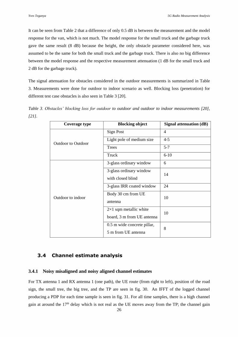
It can be seen from Table 2 that a difference of only 0.5 dB is between the measurement and the model

response for the van, which is not much. The model response for the small truck and the garbage truck

gave the same result (8 dB) because the height, the only obstacle parameter considered here, was

assumed to be the same for both the small truck and the garbage truck. There is also no big difference

between the model response and the respective measurement attenuation (1 dB for the small truck and

2 dB for the garbage truck).

The signal attenuation for obstacles considered in the outdoor measurements is summarized in Table

3. Measurements were done for outdoor to indoor scenario as well. Blocking loss (penetration) for

different test case obstacles is also seen in Table 3 [20].

Table 3. Obstacles’ blocking loss for outdoor to outdoor and outdoor to indoor measurements [20],

[21].

Coverage type Blocking object Signal attenuation (dB)

Outdoor to Outdoor

Sign Post 4

Light pole of medium size 4-5

Trees 5-7

Truck 6-10

Outdoor to indoor

3-glass ordinary window 6

3-glass ordinary window

with closed blind 14

3-glass IRR coated window 24

Body 30 cm from UE

antenna 10

2×1 sqm metallic white

board, 3 m from UE antenna 10

0.5 m wide concrete pillar,

5 m from UE antenna 8

3.4 Channel estimate analysis

3.4.1 Noisy misaligned and noisy aligned channel estimates

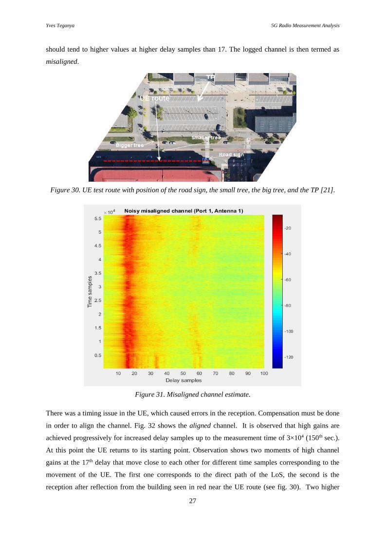
For TX antenna 1 and RX antenna 1 (one path), the UE route (from right to left), position of the road

sign, the small tree, the big tree, and the TP are seen in fig. 30. An IFFT of the logged channel

producing a PDP for each time sample is seen in fig. 31. For all time samples, there is a high channel

gain at around the 17th delay which is not real as the UE moves away from the TP; the channel gain


27

should tend to higher values at higher delay samples than 17. The logged channel is then termed as

misaligned.

Figure 30. UE test route with position of the road sign, the small tree, the big tree, and the TP [21].

Figure 31. Misaligned channel estimate.

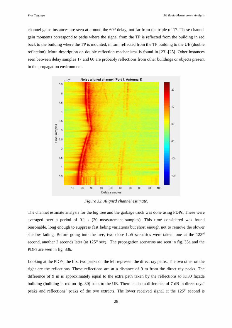
There was a timing issue in the UE, which caused errors in the reception. Compensation must be done

in order to align the channel. Fig. 32 shows the aligned channel. It is observed that high gains are

achieved progressively for increased delay samples up to the measurement time of 3×104 (150th sec.).

At this point the UE returns to its starting point. Observation shows two moments of high channel

gains at the 17th delay that move close to each other for different time samples corresponding to the

movement of the UE. The first one corresponds to the direct path of the LoS, the second is the

reception after reflection from the building seen in red near the UE route (see fig. 30). Two higher

TP

UE route


28

channel gains instances are seen at around the 60th delay, not far from the triple of 17. These channel

gain moments correspond to paths where the signal from the TP is reflected from the building in red

back to the building where the TP is mounted, in turn reflected from the TP building to the UE (double

reflection). More description on double reflection mechanisms is found in [23]-[25]. Other instances

seen between delay samples 17 and 60 are probably reflections from other buildings or objects present

in the propagation environment.

Figure 32. Aligned channel estimate.

The channel estimate analysis for the big tree and the garbage truck was done using PDPs. These were

averaged over a period of 0.1 s (20 measurement samples). This time considered was found

reasonable, long enough to suppress fast fading variations but short enough not to remove the slower

shadow fading. Before going into the tree, two close LoS scenarios were taken: one at the 123rd

second, another 2 seconds later (at 125th sec). The propagation scenarios are seen in fig. 33a and the

PDPs are seen in fig. 33b.

Looking at the PDPs, the first two peaks on the left represent the direct ray paths. The two other on the

right are the reflections. These reflections are at a distance of 9 m from the direct ray peaks. The

difference of 9 m is approximately equal to the extra path taken by the reflections to Ki30 façade

building (building in red on fig. 30) back to the UE. There is also a difference of 7 dB in direct rays’

peaks and reflections’ peaks of the two extracts. The lower received signal at the 125th second is


29

possibly due to the reflected paths shown on the lower side of fig. 33a which are destructive (out of

phase) to the direct path.

(a) (b)

Figure 33. a) Propagation scenarios (both LoS), b) PDPs at the 123rd and the 125th seconds.

3.4.2 Channel estimate analysis for the big tree blocking

The PDPs during the big tree obstruction have been extracted at different moments of the blocking (at

the seconds 138, 139, 148, and 149) as illustrated in figs. 34 and 35. The PDP for the LoS scenario at

the 123rd second before entering the tree obstruction has been added for comparison.

(a) (b)

Figure 34. a) Propagation scenarios, b) PDPs at the 123rd, 138th, and 139th seconds.


30

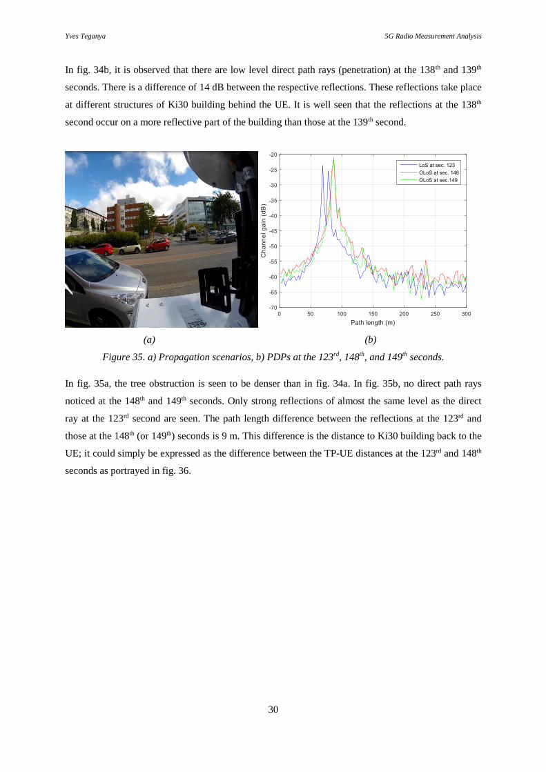
In fig. 34b, it is observed that there are low level direct path rays (penetration) at the 138th and 139th

seconds. There is a difference of 14 dB between the respective reflections. These reflections take place

at different structures of Ki30 building behind the UE. It is well seen that the reflections at the 138th

second occur on a more reflective part of the building than those at the 139th second.

(a) (b)

Figure 35. a) Propagation scenarios, b) PDPs at the 123rd, 148th, and 149th seconds.

In fig. 35a, the tree obstruction is seen to be denser than in fig. 34a. In fig. 35b, no direct path rays

noticed at the 148th and 149th seconds. Only strong reflections of almost the same level as the direct

ray at the 123rd second are seen. The path length difference between the reflections at the 123rd and

those at the 148th (or 149th) seconds is 9 m. This difference is the distance to Ki30 building back to the

UE; it could simply be expressed as the difference between the TP-UE distances at the 123rd and 148th

seconds as portrayed in fig. 36.


31

Figure 36. Reflections at the 123rd and 148th (or 149th) seconds.

3.4.3 Channel estimate analysis for the garbage truck blocking

In fig. 37b, PDPs for the LoS and OLoS by the garbage truck are shown. Ki30 building structures

remain the main source of reflections as the difference in path length with the direct path rays is 9 m.

Double reflection involving Ki30 building and the TP building is seen with other two peaks of the LoS

at path lengths of 168 m and 177 m; they are different in levels (3.5 dB), the first one is the truck-

diffracted ray while the other is only reflected on Ki30 building again. The extracts during the

blocking are seen in the same figure as well; their direct path rays occur at the same path length as the

LoS but attenuated due to diffraction around the top and side edges of the truck. Some of their

respective double-reflected components are visible but weak.

(a)


32

(b)

Figure 37. a) Some of Ki30 façade structures, b) PDPs at the 20th, 22.45, 22.55, 22.7, 23, and 23.5

seconds.

3.5 Impact on polarization and MIMO channel properties

Average channel gains over the entire bandwidth for the 4×4 MIMO paths are summarized in Table 4.

The channel gains are computed for the LoS scenario during 2.5 s.

Table 4. Average channel gains in dB of a 2.5-second long LoS scenario for the 4×4 MIMO paths.

TX

Rx

1 2 3 4

1 -19.3840 -21.1744 -17.2737 -19.3302

2 -25.7728 -25.4875 -26.2719 -26.4787

3 -16.4443 -18.9748 -16.0649 -18.4826

4 -28.1819 -25.5713 -25.2513 -25.3216

It has been found from previous work that vertically and horizontally (at both the transmitter and the

receiver) polarized or simply co-polarized waves undergo the same path loss by averaging [26], [27].

In [26], the cross-polarization between the transmitter and the receiver antennas (when the transmitting

antenna is vertically polarized and the receiving antenna horizontally polarized or vice-versa, with the


33

same radio path effect) yields to an attenuated wave compared to the co-polarization due to the

polarization mismatch loss.

Fig. 38 shows the results of the two channel pairs on the polarization analysis. The paths TX1-RX3,

TX3-RX1 are accounted for the co-polarized (vertically and horizontally) waves while the paths TX2-

RX4, TX4-RX2 are for the cross-polarization. As the ground wave component of the RF noise is

largely vertically polarized [28], it is expected that the vertically polarized wave is to be more affected

than the horizontally polarized wave. Thus, the path TX1-RX3 is for the vertical polarization and

TX3-RX1 for the horizontal polarization. The path TX2-RX4 is for the cross-polarization when the

transmitting antenna is vertically polarized, and TX4-RX2 accounts for the cross-polarization when

the transmitting antenna is horizontally polarized. It can also be seen in fig. 38 and Table 4, a

difference of 9 dB on average between the co-polarization and cross-polarization.

Figure 38. Average channel gains of a 2.5-second long LoS scenario. The paths TX1-RX3 and TX3-

RX1 are for the co-polarization. The paths TX2-RX4 and TX4-RX2 are for the cross polarization.

The average channel gains shown in figs. 39 and 40 have been computed for the road sign and the

garbage truck blocking, considering the TX and RX combinations in fig. 38.


34

Figure 39. Channel gains during the road sign blocking.

Figure 40. Channel gains during the garbage truck blocking.

In figs. 39 and 40, it should be noted that the road sign and the garbage truck blocking have a

considerable effect on the co-polarized waves than cross-polarized ones. In fig. 39, there is 0.2 s

between the dips of co-polarization effects during the blocking. With the estimated UE speed of 0.5

m/s, the distance between the blocking effects is 10 cm, which is real to be the physical separation

between antenna elements at the UE (see fig. 7).


35

4 Conclusions

This section summarizes the findings of the thesis. Moreover, it suggests possible future improvement

that could be done.

4.1 Summary of results

The measurements gathered using a 5G radio prototype have been analyzed by modelling the blocking

caused by different obstacles. The considered obstacles during this thesis are: road sign, light pole,

small bare tree, big lush tree, small truck, van, and garbage truck. It was found that:

The model response was moving close to the average of the measurement for reasonable

estimations of the obstacles’ dimensions.

For the road sign, the light pole, and the van, the model response was varying in the same

proportion as the variation in the radius of the road sign (light pole) and the width of the van.

The model response was sensitive to the height of the garbage truck. 2 % increment of the

truck height caused 20 % increment of the attenuation. This was so because the variation was

being done in regions close to the LoS scenario. This cause of sensitivity holds for the small

truck as well.

The knife-edge diffraction model was verified on the measurements. It was discovered that the

attenuation from the model was close to the attenuation in the measurements for the van, the small

truck, and the garbage truck.

The channel estimate analysis for the big lush tree was done and compared to that of a solid obstacle

(garbage truck). The signal penetration varied behind the studied tree, depending on the density of the

foliage.

On polarization and MIMO channel properties, there was a difference of 9 dB between the co-

polarized and cross-polarized paths. Furthermore, the physical separation between antenna elements at

the UE was observed on the MIMO paths when the average channel estimates during the road sign

blocking were calculated and plotted.

4.2 Future work

Modeling a tree as a screen is very simple and one could not rely much on the response from such an

assumption. Leaves move in any directions; this affects the radio wave propagation. Moisture on

leaves is also another factor that was not accounted for in the current thesis. More accurate modelling


36

of trees can be done by using computational scattering from a tree with Foldy’s approximation or

Monte Carlo Simulation for instance.

The blocking model did not include the material of the obstacle: whether reflective like metals or

dielectrics that can let the signal through. With the obstacles’ dimensions, another difference between

the small truck and garbage truck when the type of material is included in the modeling could be

observed.


37

References

[1] J. Chedia, B. Asma, and C. Belgacem, ‘‘Enabling and challenges for 5G Technologies,’’

WCITCA, 2015 World Congress on, June 2015.

[2] T. S. Rappaport et al., “Millimeter Wave Mobile Communications for 5G Cellular: It Will

Work!,” IEEE Access, vol. 1, no. 1, pp. 335-349, May 2013.

[3] G. R. MacCartney, J. Zhang, S. Nie, and T.S Rappaport, “Path loss models for 5G millimeter

wave propagation channels in urban microcells,” IEEE Globecom Wireless Commun. Symp.,

Atlanta, GA, 2013, pp. 3948-3953.

[4] B. Malila, O. Falowo, N.Ventura, “Millimeter wave small cell backhaul: An analysis of

diffraction loss in NLOS links in urban canyons,” IEEE AFRICON, 2015.

[5] Ericsson, 5G Use Cases, 2015 [Online]. Available: http://www.ericsson.com/res/docs/2015/5g-

use-cases.pdf. [Accessed: 9-Feb-2016].

[6] J. Medbo and F. Harrysson, “Channel Modeling for the Stationary UE Scenario,” 7th EUCAP,

pp. 2811-2815, 2013.

[7] METIS, ‘Final report on architecture’, 2015 [Online]. Available:

https://www.metis2020.com/wp-content/uploads/METIS_D1.4_v3.pdf. [Accessed: 9-Feb-2016].

[8] S. C. Yong, K. Jaekwon, Y. Y. Won, and G. K. Chung, MIMO-OFDM Wireless

Communications with MATLAB, John Wiley & Son (Asia) Pte Ltd, ch. 1, pp. 1-10, 2010.

[9] T. S. Rappaport, Wireless Communications Principles and Practice, 2nd ed., Englewood Cliffs,

NJ, USA: Prentice Hall, Ch. 3, p. 77, 2002.

[10] ITU, ‘Rec. ITU-R P.526-6 Propagation by diffraction’, 1999 [Online]. Available:

https://www.itu.int/dms_pubrec/itu-r/rec/p/R-REC-P.526-6-199910-S!!PDF-E.pdf. [Accessed:

15-Feb-2016].

[11] B. Sklar, “Rayleigh fading channels in mobile digital communication systems. I.

Characterization,” IEEE Commun. Mag., vol. 35, no. 9, Sept. 1997.

[12] F. Pérez Fontán and P. Mariño Espiñeira, Modeling the Wireless Propagation Channel A

Simulation Approach with MATLAB, John Wiley & Son Ltd, ch. 1, pp. 1-10, 2008.

[13] L. Ahlin, J. Zander, and B. Slimane, Principles of Wireless Communications. Studentlitteratur

AB, August 23, 2006.

[14] G.Y. Delisle, J. Lefevre, M. Lecours, and J. Chouinard, “Propagation loss prediction: A

comparative study with application to the mobile radio channel,” IEEE Trans. Veh. Technol.,

vol. 34, no. 2, pp. 86-96, May 1985.

[15] J. B. Andersen, T. S. Rappaport, and S. Yoshida, “Propagation Measurements and Models for

Wireless Communications Channels,” IEEE Commun. Mag., vol. 33, no. 1, p. 43, Jan. 1995.

http://ieeexplore.ieee.org.webproxy.student.hig.se:2048/xpl/mostRecentIssue.jsp?punumber=7352733

http://www.ericsson.com/res/docs/2015/5g-use-cases.pdf

http://www.ericsson.com/res/docs/2015/5g-use-cases.pdf

https://www.metis2020.com/wp-content/uploads/METIS_D1.4_v3.pdf

https://www.itu.int/dms_pubrec/itu-r/rec/p/R-REC-P.526-6-199910-S!!PDF-E.pdf


38

[16] Y. Okumura, E. Ohmori, and K. Fukuda, “Field Strength and its Variability in VHF and UHF

Land Mobile Radio Service,” Rev. Elec. Com. Lab, vol. 16, no. 9, 1968, pp. 825-73.

[17] M. Hata, “Empirical Formulae for Propagation Loss in Land Mobile Radio Services,” IEEE

Trans. Veh. Technol., vol. 29, no. 3, pp. 317-325, 1980.

[18] Ericsson, ‘Ericsson and Verizon 5G field trial Hits multi-Gbps speeds’, 2016 [Online].

Available: http://www.ericsson.com/news/1987883. [Accessed: 11-Apr-2016].

[19] W. Roh et al., “Millimeter-wave beamforming as an enabling technology for 5G cellular

communications: Theoretical feasibility and prototype results,” IEEE Commun. Mag., vol. 52,

no. 2, pp. 106–113, Feb. 2014.

[20] P. Ökvist et al., “15 GHz Propagation Properties Assessed with 5G Radio Access Prototype,”

2015 IEEE 26th PIMRC: Workshop on 5G Channel Measurement and Modeling, Stockholm,

2015.

[21] P. Ökvist et al., “15 GHz Street-level Blocking Characteristics Assessed with 5G Radio Access

Prototype,” in 2016 IEEE VTC - Spring, 2016.

[22] Ericsson and Keysight, ‘R1-160845 Modeling of blocking,’ [Online]. Available:

http://portal.3gpp.org/ngppapp/CreateTdoc.aspx?mode=view&contributionId=685535.

[Accessed: 11-Apr-2016].

[23] S. Mostarshedi et al., “Building Facade Homogenization in Multiple Reflection Mechanism,” in

APWC, 2011 IEEE-APS Topical Conf., pp. 1168 - 1171, Sept. 2011.

[24] M. F. Iskander and Z. Yun, “Propagation prediction models for wireless communication

systems,” IEEE Trans. Microwave Theory Tech., vol. 50, no. 3, pp. 662-673, Mar. 2002.

[25] N. Iya et al., “Ultra-wideband characterization of obstructed propagation,” in Proc. 7th IWCMC,

July 2011, pp. 624–629.

[26] H. Asplund et al., “Propagation characteristics of polarized radio waves in cellular

communications,” in Proc. IEEE 66th VTC-Fall, 2007, pp. 839–843.

[27] I. Rodriguez et al., “Analysis of 38 GHz mmWave Propagation Characteristics of Urban

Scenarios,” in Proc. European Wireless 2015; 21th European Wireless Conf., Offenbach,

Berlin, 2015, pp. 374-381.

[28] B. A. Witvliet et al., “A Novel Method for the Evaluation of Polarization and Hemisphere

Coverage of HF Radio Noise Measurement Antennas,” IEEE EMC and EMC Europe Symp.,

Dresden, Germany, Aug. 2015.

http://www.ericsson.com/news/1987883

http://portal.3gpp.org/ngppapp/CreateTdoc.aspx?mode=view&contributionId=685535


A1

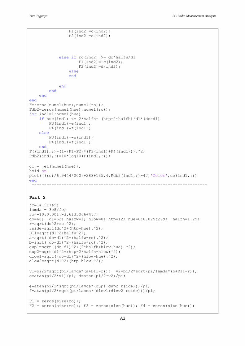
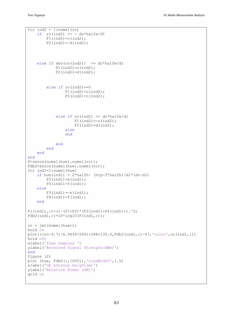
Appendix

This appendix contains the MATLAB script used in modeling the garbage truck and the model

sensitivity on the height change. All other obstacles were modeled in the same way.

Part 1

clear all close all fc=14.917e9; %Carrier frequency lamda = 3e8/fc; ro=-3.6135066:0.001:26; %Distance Range of the model plotting do=68; % TP-UE Distance; d1=62; % Obstacle-TP Distance halfw=3.3; %1/2 of the container length hlow=0; htp=12; %TP Height; hue=0:0.025:2.9; % UE height range halfh=1.25; %1/2 of the truck height

%%Computing different distances r=sqrt(do^2+ro.^2); rside=sqrt(do^2+(htp-hue).^2); D11=sqrt(d1^2+halfw^2); a=sqrt((do-d1)^2+(halfw-ro).^2); b=sqrt((do-d1)^2+(halfw+ro).^2); dup1=sqrt((do-d1)^2+(2*halfh+hlow-hue).^2); dup2=sqrt(d1^2+(htp-2*halfh-hlow)^2); dlow1=sqrt((do-d1)^2+(hlow-hue).^2); dlow2=sqrt(d1^2+(htp-hlow)^2);

v1=pi/2*sqrt(pi/lamda*(a+D11-r)); v2=pi/2*sqrt(pi/lamda*(b+D11-r));

%Computing different diffraction components c=atan(pi/2*v1)/pi; d=atan(pi/2*v2)/pi; e=atan(pi/2*sqrt(pi/lamda*(dup1+dup2-rside)))/pi; f=atan(pi/2*sqrt(pi/lamda*(dlow1+dlow2-rside)))/pi;

F1 = zeros(size(ro)); F2 = zeros(size(ro)); F3 = zeros(size(hue)); F4 = zeros(size(hue));

for ind2 = 1:numel(ro) if ro(ind2) <= - do*halfw/d1 F1(ind2)=c(ind2); F2(ind2)=-d(ind2);

else if abs(ro(ind2)) <= do*halfw/d1 F1(ind2)=c(ind2); F2(ind2)=d(ind2);

else if ro(ind2)==0


A2

F1(ind2)=c(ind2); F2(ind2)=c(ind2);

else if ro(ind2) >= do*halfw/d1 F1(ind2)=-c(ind2); F2(ind2)=d(ind2); else end

end end end end F=zeros(numel(hue),numel(ro)); Fdb2=zeros(numel(hue),numel(ro)); for ind1=1:numel(hue) if hue(ind1) <= 2*halfh- (htp-2*halfh)/d1*(do-d1) F3(ind1)=e(ind1); F4(ind1)=f(ind1); else F3(ind1)=-e(ind1); F4(ind1)=f(ind1); end F((ind1),:)=(1-(F1+F2)*(F3(ind1)+F4(ind1))).^2; Fdb2(ind1,:)=10*log10(F(ind1,:));

cc = jet(numel(hue)); hold on plot(((ro)/6.9444*200)+288+135.4,Fdb2(ind1,:)-47,'Color',cc(ind1,:)) end -----------------------------------------------------------------------

Part 2

fc=14.917e9; lamda = 3e8/fc; ro=-10:0.001:-3.6135066+4.7; do=68; d1=62; halfw=1; hlow=0; htp=12; hue=0:0.025:2.9; halfh=1.25; r=sqrt(do^2+ro.^2); rside=sqrt(do^2+(htp-hue).^2); D11=sqrt(d1^2+halfw^2); a=sqrt((do-d1)^2+(halfw-ro).^2);

b=sqrt((do-d1)^2+(halfw+ro).^2); dup1=sqrt((do-d1)^2+(2*halfh+hlow-hue).^2);

dup2=sqrt(d1^2+(htp-2*halfh-hlow)^2); dlow1=sqrt((do-d1)^2+(hlow-hue).^2);

dlow2=sqrt(d1^2+(htp-hlow)^2);

v1=pi/2*sqrt(pi/lamda*(a+D11-r)); v2=pi/2*sqrt(pi/lamda*(b+D11-r)); c=atan(pi/2*v1)/pi; d=atan(pi/2*v2)/pi;

e=atan(pi/2*sqrt(pi/lamda*(dup1+dup2-rside)))/pi; f=atan(pi/2*sqrt(pi/lamda*(dlow1+dlow2-rside)))/pi;

F1 = zeros(size(ro)); F2 = zeros(size(ro)); F3 = zeros(size(hue)); F4 = zeros(size(hue));


A3

for ind2 = 1:numel(ro) if ro(ind2) <= - do*halfw/d1 F1(ind2)=c(ind2); F2(ind2)=-d(ind2);

else if abs(ro(ind2)) <= do*halfw/d1 F1(ind2)=c(ind2); F2(ind2)=d(ind2);

else if ro(ind2)==0 F1(ind2)=c(ind2); F2(ind2)=c(ind2);

else if ro(ind2) >= do*halfw/d1 F1(ind2)=-c(ind2); F2(ind2)=d(ind2); else end

end end end end F=zeros(numel(hue),numel(ro)); Fdb2=zeros(numel(hue),numel(ro)); for ind1=1:numel(hue) if hue(ind1) < 2*halfh- (htp-2*halfh)/d1*(do-d1) F3(ind1)=e(ind1); F4(ind1)=f(ind1); else F3(ind1)=-e(ind1); F4(ind1)=f(ind1); end

F((ind1),:)=(1-(F1+F2)*(F3(ind1)+F4(ind1))).^2; Fdb2(ind1,:)=10*log10(F(ind1,:));

cc = jet(numel(hue)); hold on plot(((ro-4.7)/6.9444*200)+288+135.4,Fdb2(ind1,:)-47,'Color',cc(ind1,:)) hold off xlabel('Time Samples ') ylabel('Received Signal Strength(dBm)') end figure (2) plot (hue, Fdb2(:,10001),'LineWidth',1.5) xlabel('UE Antenna height(m)') ylabel('Relative Power (dB)') grid on

5G Radio Measurement Analysis - DiVA...

Documents

Transcript of 5G Radio Measurement Analysis - DiVA...