550.448 Assignment Financial Engineering and …daudley/448/jhuonly/550.448 SP14 Wk4 (CF...

1

550.448Financial Engineering and

Structured Products

Week of February 17, 2014Cash Flows,

Static Valuation & Credit Elements for Structured Finance

1.1 1.2

Assignment

Reading Read Chapters 4 & 5 of R&R Allman: Introduction and Chapters 1-2 Allman: Chapter 3-4 (next)

Assignment See Website (2 problems) Problem 1 due next Wednesday (February 26) Problem 2 due on Monday, March 3

1.3

Assignment

Last day of Class – Wednesday, April 31st

Final Exam Tuesday, May 13, 2pm-5pm Whitehead 304

1.4

Plan for This Week

The Corporate Structure for Securitization Finish-Up

Allman Chapter 1-2 Material Static Valuation Model (BOTE) Elements of Credit Analysis for Structured

Finance

2

1.5

Deconstructing the Corporation

The Context for Describing Operations and Operational Risk Structured Finance Micro-Market Timely incremental movements of cash through accounts in the

payment system Risks associated w/corresponding title/custody arrangements

governed under the indenture

Macro Market Relationship between Buyers Sellers Others (Agents, Professional support, Regulators and Data Vendors)

1.6


The Context for Describing Operations and Operational Risk Meta (Macro) Market Mesh of Credit, Operating, and Governance systems Through which Structured Transactions flow Changing the velocity of money Transforming the structures of capital & risk

1.7


Market Micro-Structure Operation Servicing an amortizing loan pool is simple, compared to operating

a corporation Enables the true sale SPE (QSPE under FASB 140) to be

amenable to rule-based governance and automation Fortunate for the borrower as it facilitates the capture of cost-of-funds arbitrage

SPE is structured to satisfy bankruptcy-remoteness with rigorous constraints on scope of operations – the funding “machine” Servicers, trustees, custodians, swap counterparties are the proverbial cogs in

the machine

1.8


Market Micro-Structure Constitution: The Pooling and Servicing Agreement The most important operational document is the PSA Spells out precisely how to Segregate cash inflows from the general accounts of the seller/servicer Set up trust accounts And to whom funds of the trust are distributed, including for reinvestment

All important to analysis when modeling the deal because it is the definitive, contractually binding transaction structure

3

1.9


Market Micro-Structure Payment Mechanics Account structure enforces segregation of collections from the

servicer/seller by passing the receivables directly into a trust account owned by the SPE

Following the Money – The Time Line Record Date – end of each collection period Collection Period (usually, 1 month) Collection Account & the daily sweep – nothing is left exposed

Determination Date (focus on the asset side of SPE balance sheet) Servicer summarizes the most recent collection period: interest, penalty interest,

principal, prepays, delinquencies, defaults/recoveries, surety bond payments, etc.

1.10


Market Micro-Structure Following the Money – The Time Line (continued) Calculation Date (focus on the liability side of SPE balance sheet) Servicer establishes the amounts due bond holders and all third parties as a

consequence of the Determination Includes trigger provisions, reserve/spread accounts, etc

Distribution Date Servicer passes the amounts Calculated to the paying agent with payment

instructions to pay the ultimate recipients

Payment Date Amounts sitting in the various sub-accounts are wired to their intended recipients

(servicer, note holders, trustee, etc)

1.11


Market Micro-Structure Primary Market & the Closing Lien on title is transferred to issuer in exchange for cash at closing Investors receive the notes in exchange for cash at closing

3rd Parties not in flow

• IB: advisor, underwriting, distribution (commission)• Lawyers: Opinions (TS & NC) + Documents (fees)• Accountants (fees)• Ratings Agencies (commission)

1.12


Market Micro-Structure Operational Flows

3rd Parties not in flow

• Ratings Agencies (annual fee)• Mark-to-market Advisories• Data Vendors

• Data from trustee• Clean & normalize• Publish in raw form or with value-add

4

1.13


Market Macro-Structure Buyers Sellers – Originator, (Transferor), Issuer (SPE) Agents Intermediaries bringing buyer & seller together Collateral Managers/Servicers/ Program Administrators Custodians/Trustees Clearing & Settlement Agents Issuing & Paying Agents

Professional Services – Lawyers & Accountants Regulators Data Vendors 1.14


More About Agents Arranging the Transaction (prior to Origination) An Investment/Commercial Bank Placement Underwriting/Structuring the Transaction

Structuring: Creating the design for redistributing the risks of the pool across different classes of securities According to prevailing market risk/return demands Meeting investor appetite In “compliance” with rating agency criteria As the underwriter may become an investor, has the potential to represent both

sides of the transaction

Servicer – Sell-side allegiance Trustee – Buy-side allegiance

1.15


More About Agents Clearing Agent – collects funds and verifies transaction information Settlement Agent – Finalizes sale and oversees transfer of ownership

from seller to buyer Data Vendors – Huge, new role in supporting this market Aggregation and transmission of performance data (servicer reports) and trustee

reports Describing the “state” of a transaction adds value

1.16


Market Meta-Structure: To Build A Better Model Nationally Recognized Statistical Rating Organization

(NRSRO) SEC-licensed credit rating agency Designs contracts for off-balance sheet financing Focus is on primary issuance Little support for secondary trading

What is in the future?

Over the Counter Market Can this be improved?

5

1.17

Questions?

Now to Allman

Asset Cash Flow Generation

Cash Flow (CF) Structure/Model for Assets We begin with CF into the structure – Asset CF Generation In general include interest, principal (both scheduled and

unscheduled – prepayment of principal), defaults, and recoveries Notional Asset CF – CF without giving affect to prepayments and

defaults Questions: How will the assets exist over time? What and how much data exists for the assets?

Depending on the answers to the questions we will consider Loan level generation of CF, or Representative Line generation

1.18


Loan Level vs. Representative Line How do the assets exist over time? The assets in a structured transaction are static (loans in pool

don’t change) or they can revolve

For a static pool, loan level analysis is preferred Now, what information exists? Detailed data required on each loan for Loan Level Analysis (LLA) If this is not the case, then Representative Line Analysis (RLA) is

an alternative (think MBS pass-through securities – not so horrible)

Either way, cash flows can be generated However, the more diverse a pool, the more distorted the

result from Representative Line Analysis See example: Rep_Lines.xls in Ch 02 Additional Files Folder1.19


Loan Level vs. Representative Line Analysis Again, how do the assets exist over time? If the assets are revolving, the Representative Line Analysis

seems more appropriate

Representative Line Analysis works best if the eligibility criteria for revolving collateral is narrowlydefined and strictly adhered-to In any event, we always assume that the eligibility criteria is

fulfilled with the worst collateral that meets the criteria

Decision Tree Revolving Pool? Yes. Use Representative Line Analysis

1.20

6


Loan Level vs. Representative Line Analysis Decision Tree Revolving Pool? Yes. Use Representative Line Analysis

Revolving Pool? No Is Loan Level Data Available? Yes. Use Loan Level Analysis No. Use Representative Line Analysis

Model Builder PMB uses single Representative Line Analysis Useful to get started For more elaborate LLA or for multiple line RLA, simple VBA

enhancements remedy the situation 1.21

Asset Cash Flow Generation – Model Builder

The Input sheet for asset CF generation The single representative line is based on a pool that

pays interest and principal; includes as a minimum Original balance & Current balance Interest Rate Original Term & Remaining Term Additional (general case of assets’ yield off floating rate)

Fixed Rate Amortization CF are created by 1st calculating the level payment using PMT Interest for period results from the period’s beginning balance Subtract interest from payment gives period’s principal payment Subtract period’s principal from beginning balance gives

period’s ending balance 1.22


The Input sheet for asset CF generation Floating Rate Amortization While most deals have fixed rate collateral, a significant number

are floating based; since more complex, we must be general enough in our approach to handle these

Additional Attributes of Floating rate Collateral Rate Index and Margin Lifetime Rate Cap and Floor Periodic Rate Cap and Floor Rate Reset Frequency and First Reset Date

The forward projecting assumption for the underlying index primarily drives the interest calculation

1.23


The Input sheet for asset CF generation Floating Rate Amortization Prime consideration for Floating rate Amortization is how the CF

is affected with rate changes Either payment changes or term of the loan changes

Index off which the assets are based becomes yet another attribute to cause the need for multiple representative lines –one for each index

Organizing the indexes is the final point Each index is a projected vector of rates as long as the number of

periods (up to 360) Storing in the input sheet would be inefficient – so we create a

separate sheet for vectors

1.24

7


The Cash Flow sheet for asset CF generation This is where the calculations for asset CF generation

take place When using the representative Line methodology, the

Notional Schedule of amortization needs to be created Called notional because it does not take into account

prepayments, defaults or recoveries Later, these aspects will be incorporated to create the actual

amortization schedule

The notional schedule of amortization uses 6 columns1) Beginning Balance 4) Interest2) Periodic Interest Rate 5) Principal3) Payment 6) Ending Balance 1.25


The Cash Flow sheet for asset CF generation Look at the Model Builder MB2.2 for illustration Stress rate curves can be entered for individual vectors

or forward curves from another source Here is where certain Monte Carlo Analyses start

1.26

1.27

Static Valuation Model

BOTE: A Static self-consistent Valuation tool Premise of Securitization To employ capital more efficiently use financial assets rather than

the entire balance sheet to raise working capital Paradigm shift in financing – allows a company to grow and prosper

at the speed of its own success, but only when Firm is financially solvent Diversified Financial Asset base – pooled payment risk of assets is less than firm To grow, firm needs working capital locked up in its assets Market understands value proposition of off-balance sheet financing

Securitizations are a special type of structured finance transaction whereby the funding arbitrage is achieved by transferring financial assets off-balance-sheet (with transparency and disclosure) through a well-designed capital structure 1.28


BOTE: A Static self-consistent Valuation tool Back-of-the-envelope (BOTE) refers to the original, semi-

self-consistent approach used for structured securities Self-consistent because the valuation draws information about the

transaction directly from the transaction’s performance data Semi-self-consistent at the outset as loss expectations are derived

from peer transactions Fully-self-consistent to the extent actual performance progress is

incorporated into the analysis

BOTE came into existence in the 80s Now replaced by more sophisticated approaches that incorporate

time and uncertainty in transaction value and risk Yet, still useful in quick look analysis and in defining a taxonomy

8

1.29


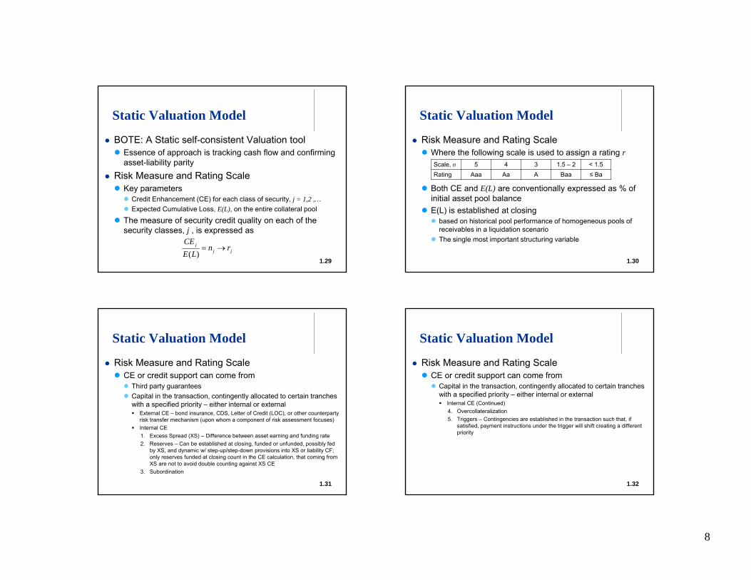
BOTE: A Static self-consistent Valuation tool Essence of approach is tracking cash flow and confirming

asset-liability parity Risk Measure and Rating Scale Key parameters Credit Enhancement (CE) for each class of security, j = 1,2 ,… Expected Cumulative Loss, E(L), on the entire collateral pool

The measure of security credit quality on each of the security classes, j , is expressed as

( )j

j j

CEn r

E L

1.30


Risk Measure and Rating Scale Where the following scale is used to assign a rating r

Both CE and E(L) are conventionally expressed as % of initial asset pool balance

E(L) is established at closing based on historical pool performance of homogeneous pools of

receivables in a liquidation scenario The single most important structuring variable

Scale, n 5 4 3 1.5 – 2 < 1.5Rating Aaa Aa A Baa ≤ Ba

1.31


Risk Measure and Rating Scale CE or credit support can come from Third party guarantees Capital in the transaction, contingently allocated to certain tranches

with a specified priority – either internal or external External CE – bond insurance, CDS, Letter of Credit (LOC), or other counterparty

risk transfer mechanism (upon whom a component of risk assessment focuses) Internal CE

1. Excess Spread (XS) – Difference between asset earning and funding rate2. Reserves – Can be established at closing, funded or unfunded, possibly fed

by XS, and dynamic w/ step-up/step-down provisions into XS or liability CF; only reserves funded at closing count in the CE calculation, that coming from XS are not to avoid double counting against XS CE

3. Subordination

1.32


Risk Measure and Rating Scale CE or credit support can come from Capital in the transaction, contingently allocated to certain tranches

with a specified priority – either internal or external Internal CE (Continued)

4. Overcollateralization5. Triggers – Contingencies are established in the transaction such that, if

satisfied, payment instructions under the trigger will shift creating a different priority

9

1.33


Transaction Analysis Consider the a priori data for a hypothetical transaction

1.34


Transaction Analysis The 2 classes can be rated through the following steps Determine the maximum amount of CE available to each class Reduce the maximum to a certainty-equivalent amount Compute ratio of CE to E(L) Determine rating from scale

The CE available to each class is, in order of liquidityClass A Class B

Excess Spread (XS) Excess Spread (XS)Reserve Account – 1% Reserve Account – 1%

Subordination – 10% NA

1.35


Transaction Analysis (Naïve) Reserve funding and subordination can be read right from

the term sheet – not so with XS Depends on defaults and prepayments which materialize over time

– conundrum for the static BOTE method Must be estimated as a maximum and then reduced to an informed

certainty-equivalent amount First step in computing XS is to compute gross spread (GS)

So considering 5-year term the total XS is, 14 1 7.3 5.7%GS WAC SF WAI

5 5.7 28.5%XS

1.36


Transaction Analysis (Naïve) So we have the ratings

The flaw – amortization not taken into account, GS is not received for full 5-years on total amount outstanding at closing

10

1.37


Transaction Analysis (Accounting for Amortization) Using average life (AL) concept – maturity of bullet-maturity equivalent

With P0 as initial principal balance, periodic interest rate r, maturity T, and dp(t) as the principal amortization schedule; average life is

Yields 0

0

1 1( ) 33.45 2.8ln 11 1

TaT

Tt tdp t mo yearsP rr

2.8 5.7 16.0% (not 28.5%)XS 1.38


Transaction Analysis (A Better Certainty-Equivalent) Three adversities that further effect XS Elevated Prepayments Adverse Prepayments Timing of receipt of XS vs. timing of losses

Elevated Prepayments (example of 100% to 200%) Requires a CF model to track XS under elevated speeds

1.39

Static Valuation Model Elevated Prepayments (example of 100% to 200%)

1.40


Transaction Analysis (A Better Certainty-Equivalent) Adverse Prepayments Even if forecast prepayments materialize, the composition of

prepayments and defaults is such that loans with above average coupon rates are more likely to refinance or default Hence income from them cannot be counted upon

A stress test that can be carried out assumes that the top 20% of the loans by APR drop out at time zero Measure the reduction on WAC, multiply by AL and subtract from total XS See next slide

11

1.41


Transaction Analysis (A Better Certainty-Equivalent) Adverse Prepayments

1.42


Transaction Analysis (A Better Certainty-Equivalent) Timing of receipt of XS vs timing of losses XS is most abundant at the outset of the transaction Losses typically occur later in the transaction life-cycle A material portion of the XS may leave the structure before it is

needed/utilized Issuers want provisions to return unneeded XS before the end of the life-cycle

and if so released, there is a net reduction in XS availability later on This is XS that if not used will be lost back to the issuer – use-it-or-loose-it (UIOLI) This amount should be calculated and accounted for

1.43


Transaction Analysis (A Better Certainty-Equivalent) So taking these 3 elements into account, what is the better

“certainty-equivalent” CE that remains Given the 5% E(L), the earlier determined XS (AL adjusted) would

be reduced further by 2% for elevated prepayments 0.67% annual for adverse prepayments (=> 0.67 x 2.8 = 1.88) And 4.33% for UIOLI

This leaves XS = 16 – 2 – 1.88 – 4.33 = 7.8% Where the 16% is the XS with just the average life adjustment

Class A CE = 7.8 + 1 + 10 = 18.8 => CE/E(L) = 20/5 = 3.76 => Rating Aa

Class B CE = 7.8 + 1 = 8.8 => CE/E(L) = 8.8/5 = 1.76 => Rating Ba1.44


Shortcomings of the BOTE Analysis It is only for investment-grade tranches ( ≥ BBB/Baa ) It portrays an integer scale and assigns the CE/E(L) to a

rating in a somewhat arbitrary way (rounding) Most important, it does not accommodate time or

uncertainty (probability) Time in that CE is measured at closing (t=0) Loss, E(L) is measured at maturity (t=T) An approach that recognizes time would keep track of evolving

losses/prepayments and the impact on evolving CE Recognizing uncertainty would incorporate deviations from an

expected evolution of loss

12

1.45

Elements of Credit Assessment

Sources of Credit Judgment and Intuition Identifying salient drivers of a transaction and synthesizing

them into credit understanding & insight Reference Materials that support this include Source

Material on: Structure of Individual Transactions and their historical performance Assets to be securitized and their historical performance Methods used to assess the transaction’s payment certainty

Source Material on the Transaction Structure In addition to PSA … Prospectus and Offering Memorandum or Circular

1.46


Source Material on the Transaction Structure Accessible Summary of the Transaction Cover Page of Prospectus Size (how much is being raised) and Date of Initial Offering (Closing) Tranche Description: Name, Size, Coupon, Maturity, Price, Average Life, Rating Disclosure: Underwriter, Advisors, external CE providers, other parties Provides key data from which capital structure and from which deterministic CE

can be calculated – subordination, overcollateralization, reserve funds, spread accounts, yield supplements, etc.

If any tranches will be allotted outside the offering, these should be disclosed

Term Sheet (at front of Prospectus) Discloses how the transaction is intended to work Focuses on liabilities: Capital Structure, CE & pay down mechanics Little asset-side static pool data, though AB requires disclosure of issuer static

pool history (helpful, but does not complete E(L) expectation into Prospectus)

1.47


Source Material on the Transaction Structure Accessible Summary of the Transaction Transaction Analysis Uses BOTE method for reviewing credit pieces Workable using incomplete specification Allows backing-out of E(L) used for rating

Transaction Analysis (Example) – Consider Cover Page Liability

1.48


Source Material on the Transaction Structure Accessible Summary of the Transaction Backing Out Implied E(L) Assuming no reserve, zero XS and approximating the rating factor Class A has 15% subordination => 15/5 = 3 = E(L) Similarly for other classes (B: 8.5/2.8 = 3 = E(L) Equity is 3.5% so residual CF is expected to be .5%

13

1.49


Source Material on the Transaction Structure Accessible Summary of the Transaction With ex ante collateral analysis, E(L) = 2.5% & Restating For the A Class: 15/2.5 = 6 => better credit & lower risk premium of .25%

Economic Arbitrage (for doing extra analysis on the collateral) For Class A: 0.35 – 0.25 = 0.10 over an average life of 2.5 years = 25 bps

1.50


History of Structural Convergence Until mid-1990s: Deals mostly consisted of Sequential-pay credit tranches and static reserve funds

In mid-1990s, resultant over-collateralization is redressed: Triggers more finely sculpt the waterfall while still defending against

payment uncertainty

In early 2000s, spread compression, rising prepayment risk & aggressive use of prefunding allowed/encouraged: Subclasses of money-market and term notes of staggered maturity Use of here-to-fore agency CMO tranche structures PAC, TAC, IO/PO, Z-class etc.

Where are we today? We have to go back to the collateral

1.51


Credit risk in the SPE is the main Structural Driver Source of comprehensive analysis: vintage, static pool Vintage: loans by same originator w/homogeneous seasoning Within vintages, underwriting characteristics are merged into a

basic unit of analysis – the static pool To avoid selection bias, pooling should proceed by a random

selection of loans underwritten to a uniformly applied loan policy

Once a pool-cut is available, the most important single measure is the cumulative loss on the pool, E(L) An E(L) that is properly determined can be placed in an envelope of

capital protection (CE) that mitigates risk to security value over the life of risk exposure to loss

But, what is Loss? 1.52


Loss Lifecycle : Delinquency, Default, Loss & Recovery

Rows: t-1 ; Columns: t

14

1.53


Loss Lifecycle : Delinquency, Default, Loss & Recovery Delinquency can cure, but only when obligor has made all

payments currently due – not entirely so, today (beware) Called: “recency” – if a payment is made or otherwise ordained

The Empirical Loss Curve Basis of Expected Loss Analysis Loss occurrence does not move linearly across time Rather an S-shaped unfolding of losses Called the static pool loss curve or just loss curve

Vintage loss curves – assets of different risk grades from different lenders where, after a while they become iconic


The Empirical Loss Curve Industry vs. Issuer Loss Curve Cumulative principal losses likely to occur in pool of loans S-Curve to principal that pool is likely to loose in total Ideally, issuer specific for specific collateral pool

Factors driving Loss Curve Asset importance to borrower Borrower creditworthiness Asset value in secondary market (LTV) Terms of the loan and term to maturity

1.54


The Empirical Loss Curve

1.55Automobile Loss Curve: Principal Losses at 10% (Hypothetical)


The Empirical Loss Curve

1.56Hypothetical Curve Showing the Borrowers Equity Position

15

1.57


The Empirical Loss Curve Issuer Loss Curves are the basis of predicting future

losses on new transactions Practice originated with agencies With insufficient data, peer issuer curves can be used

Loss Curves may be constructed in a spreadsheet Using an issuers vintage data, an average or base curve is built Data may be “cloned” to take advantage of all available data

1.58


The Empirical Loss Curve Base Curve Construction

1.59


The Empirical Loss Curve New Loss Curve for Deal under Analysis is derived from a

Consecutive Sequence of Vintage curves believed to be Representative of how the New Transaction will Perform From this series an average curve is computed which becomes the

base curve for the new transaction Base Curve is normalized between 0 and 1 Each point is interpreted as the time-dependent ratio of current to

ultimate loss Cloning Data of Different Vintages


The Empirical Loss Curve – Cloning Data Additive Method

Multiplicative Method (similar nomenclature to above)

1.60

1 1

Base Curve: , 1, 2,...,Target Curve: , 1, 2,..., ;To Complete: ( ), 1, 2,...,Cumulative Expected Loss Estimate for the Pool: ( ) ( )

i

i

i i i i

n N n

y i Ng i n n Ng g y y i n n N

E L g y y

11

1 1

Base Curve: , 1, 2,...,Target Curve: , 1, 2,..., ;

To Complete: , 1, 2,...,

Cumulative Expected Loss Estimate for the Pool:

( )

i

i

ii i

i

Ni

N nn i

y i Ng i n n N

yg g i n n Ny

yE L g gy

16


The Empirical Loss Curve – Cloning Data Cloning Data - See Table on next slide Quarterly Data Is the Loss Curve Complete? Does it show the characteristic saturation/tapering?

How do we bootstrap to use all available vintage data Use first curve to complete second – a composite – not an average Use both additive and multiplicative methods to cross verify range Then complete 2XX2-2

Considerations for Loss Curve Development How much history is relevant Do issuers stay the same or go “down market”

Composite for several issuers1.61


The Empirical Loss Curve – Cloning Data

1.62Issuer’s (hypothetical) Loss Curve History


The Empirical Loss Curve – Cloning Data

1.63

Projecting or Cloning the (hypothetical) Loss Curve

1.64


The Empirical Loss Curve Accounting for Recoveries – Three Methods Cash Basis: Recognition of Losses & Recoveries When they Occur Accrual Basis: Match inflow to outflow by attributing them to the

same period Estimated Basis: Netting a constant percentage of recoveries from

gross loss with an episodic true-up

Cash Basis is the only one that takes the true time value of money into account

17

1.65


Loss Curves & Loss Distributions Loss Distribution adds the standard deviation of losses to the expected loss

1.66


Payment Certainty vs. Value This is the fundamental premise in financial analysis Corporate Finance Analysis employs proxies of value (e.g.,

financial statement ratios) where a link to value is established via a mapping process Similarly, such an approach exists in structured finance with the

Benchmark Pool Method Usually the approach for markets that are yet to mature and then is

superseded with maturity Benchmark Pool method assumes a cash flow characteristic, given

a Benchmark Pool, for which there is little empirical validation CDO market is one example

1.67


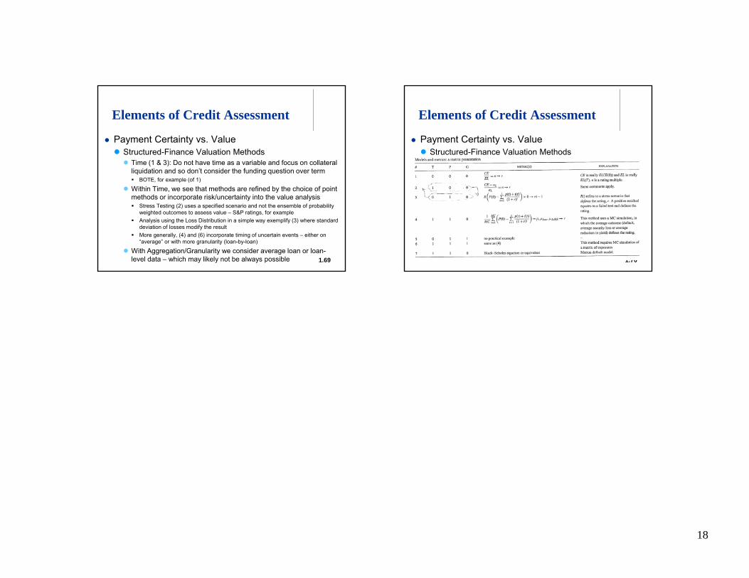
Payment Certainty vs. Value Structured-Finance Valuation Methods use direct value

inputs: interest, loss, default, recovery, delinquency, principal balance, time-to-maturity, yield, time, etc. The main variations in valuation methods explore 3 dimensions Time/Timeless Probabilistic/Certain Aggregated/Granular

As an Aside – An alternative paradigm embodies Merton’s Model for explicit default probability estimation

A taxonomy for method comparison is shown following

1.68


Payment Certainty vs. Value Structured-Finance Valuation Method

18

1.69


Payment Certainty vs. Value Structured-Finance Valuation Methods Time (1 & 3): Do not have time as a variable and focus on collateral

liquidation and so don’t consider the funding question over term BOTE, for example (of 1)

Within Time, we see that methods are refined by the choice of point methods or incorporate risk/uncertainty into the value analysis Stress Testing (2) uses a specified scenario and not the ensemble of probability

weighted outcomes to assess value – S&P ratings, for example Analysis using the Loss Distribution in a simple way exemplify (3) where standard

deviation of losses modify the result More generally, (4) and (6) incorporate timing of uncertain events – either on

“average” or with more granularity (loan-by-loan)

With Aggregation/Granularity we consider average loan or loan-level data – which may likely not be always possible 1.70


Payment Certainty vs. Value Structured-Finance Valuation Methods

550.448 Assignment Financial Engineering and …daudley/448/jhuonly/550.448 SP14 Wk4 (CF...

Documents

Transcript of 550.448 Assignment Financial Engineering and …daudley/448/jhuonly/550.448 SP14 Wk4 (CF...