523 Assignement (Completed) Assg # 02

8/13/2019 523 Assignement (Completed) Assg # 02

http://slidepdf.com/reader/full/523-assignement-completed-assg-02 1/13

Table of Contents

Time Series Analysis (TSA) ............................................................................................................................ 1

Components of TSA: ..................................................................................................................................... 1

Trend Component: .................................................................................................................................... 2

Cyclical Component: ................................................................................................................................. 2

Seasonal Component: ............................................................................................................................... 2

Irregular Component: ............................................................................................................................... 3

Decomposition: ............................................................................................................................................. 3

Trend: ............................................................................................................................................................ 3

Trend Curves: ................................................................................................................................................ 4

Seasonal Variation: ....................................................................................................................................... 4

Ratio-to-Moving Average: ............................................................................................................................. 5

Car Registrations ....................................................................................................................................... 5

Seasonally Adjusted Data:............................................................................................................................. 5

Cyclical Variation: .......................................................................................................................................... 6

Economic Indicators: ..................................................................................................................................... 7

Cyclical Cautions: .......................................................................................................................................... 7

Long Term Forecasts: .................................................................................................................................... 8

Cyclical and Irregular Effects: ........................................................................................................................ 8

Outboard Sales Example: .............................................................................................................................. 8

Seasonal Forecasting: ................................................................................................................................... 9

Case Study: .................................................................................................................................................... 9

Implementing the Model: ........................................................................................................................... 10

Using optimal values for α and ß that minimizes the MSE: ........................................................................ 10

Forecasting with Holt’s Model: ................................................................................................................... 10

SWOT ANALYSIS: ......................................................................................................................................... 11

STRENGHT: .............................................................................................................................................. 11

WEAKNESS: ............................................................................................................................................. 11

OPPORTUNITY: ........................................................................................................................................ 11

THREAT: ................................................................................................................................................... 11

Conclusion: .................................................................................................................................................. 12

Recommendation:....................................................................................................................................... 12



1 | P a g e

Time Series Analysis (TSA)

“The Art of Forecasting”

Time series are analyzed to discover past patterns of variability that can be used to

forecast future values.

A time-series is a set of observations on a quantitative variable collected over time.

Examples

Dow Jones Industrial Averages

Historical data on sales, inventory, customer counts, interest rates, costs, etc.

Businesses are often very interested in forecasting time series variables.

Often, independent variables are not available to build a regression model of a time

series variable.

In time series analysis, we analyze the past behavior of a variable in order to predict its

future behavior

Decomposition - identify components that influence the series.

Trend

Cyclical

Seasonal

Irregular

Components of TSA:

• Cycle

– An up-and-down repetitive movement in demand.

– repeats itself over a long period of time

• Seasonal Variation

– An up-and-down repetitive movement within a trend occurring periodically.

– Often weather related but could be daily or weekly occurrence

• Random Variations



2 | P a g e

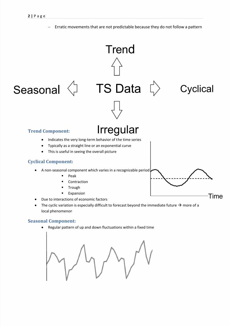
Trend

Seasonal Cyclical

Irregular

TS Data

– Erratic movements that are not predictable because they do not follow a pattern

Trend Component:

Indicates the very long-term behavior of the time series

Typically as a straight line or an exponential curve

This is useful in seeing the overall picture

Cyclical Component:

A non-seasonal component which varies in a recognizable period Peak

Contraction

Trough

Expansion

Due to interactions of economic factors

The cyclic variation is especially difficult to forecast beyond the immediate future more of a

local phenomenon

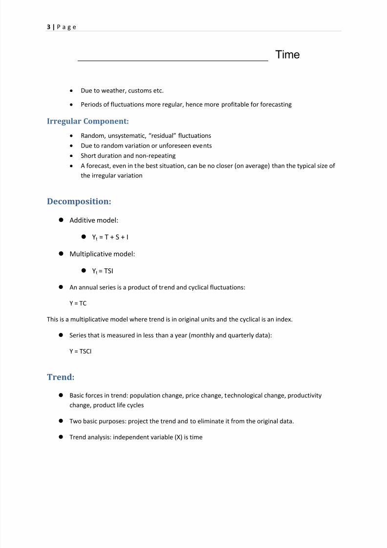
Seasonal Component:

Regular pattern of up and down fluctuations within a fixed time

Tim



3 | P a g e

Due to weather, customs etc.

Periods of fluctuations more regular, hence more profitable for forecasting

Irregular Component:

Random, unsystematic, “residual” fluctuations

Due to random variation or unforeseen events

Short duration and non-repeating

A forecast, even in the best situation, can be no closer (on average) than the typical size of

the irregular variation

Decomposition:

Additive model:

Yt = T + S + I

Multiplicative model:

Yt = TSI

An annual series is a product of trend and cyclical fluctuations:

Y = TC

This is a multiplicative model where trend is in original units and the cyclical is an index.

Series that is measured in less than a year (monthly and quarterly data):

Y = TSCI

Trend:

Basic forces in trend: population change, price change, technological change, productivity

change, product life cycles

Two basic purposes: project the trend and to eliminate it from the original data.

Trend analysis: independent variable (X) is time

Time



4 | P a g e

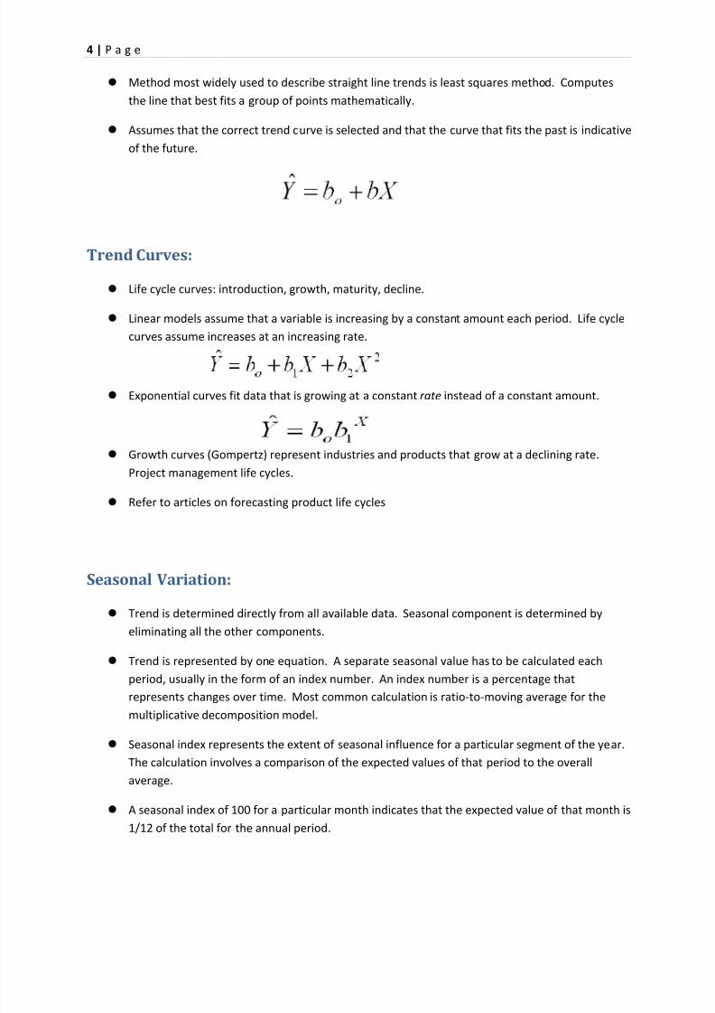
Method most widely used to describe straight line trends is least squares method. Computes

the line that best fits a group of points mathematically.

Assumes that the correct trend curve is selected and that the curve that fits the past is indicative

of the future.

Trend Curves:

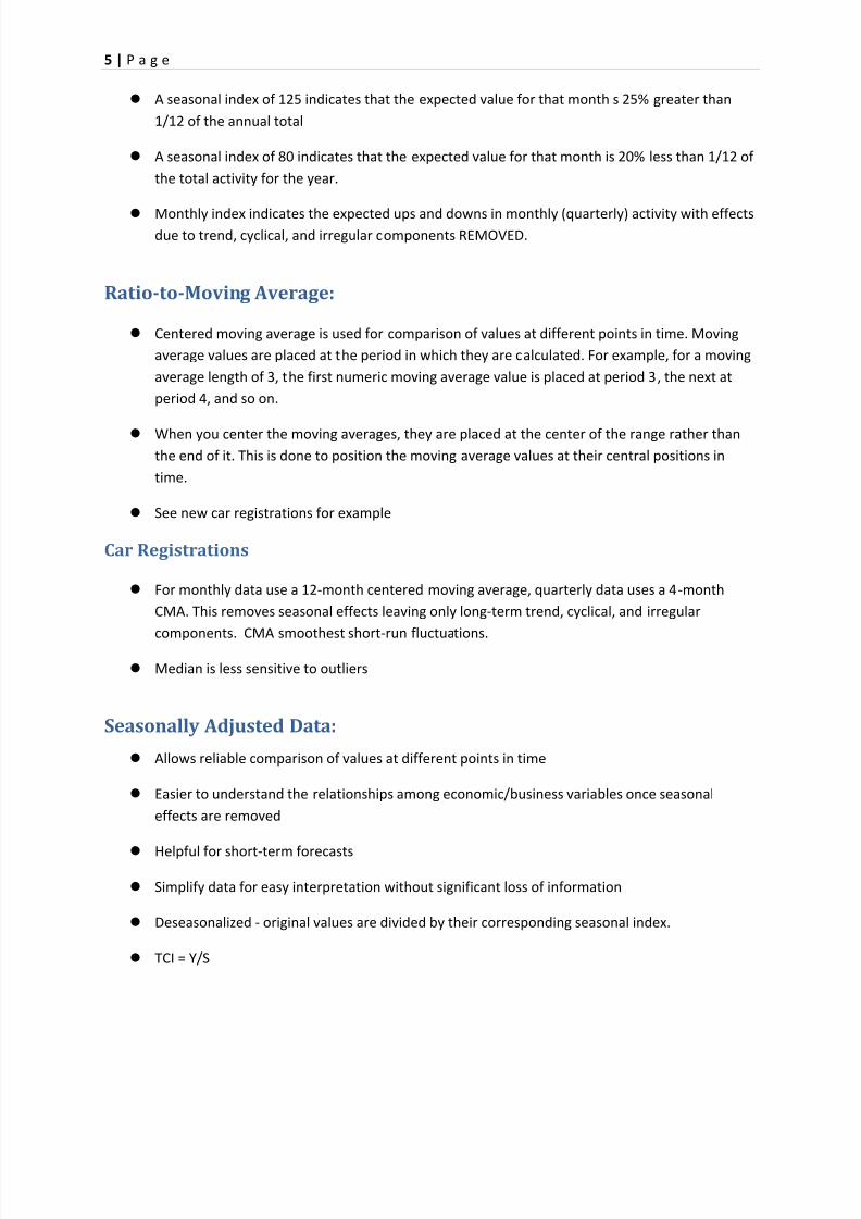
Life cycle curves: introduction, growth, maturity, decline.

Linear models assume that a variable is increasing by a constant amount each period. Life cycle

curves assume increases at an increasing rate.

Exponential curves fit data that is growing at a constant rate instead of a constant amount.

Growth curves (Gompertz) represent industries and products that grow at a declining rate.

Project management life cycles.

Refer to articles on forecasting product life cycles

Seasonal Variation:

Trend is determined directly from all available data. Seasonal component is determined by

eliminating all the other components.

Trend is represented by one equation. A separate seasonal value has to be calculated each

period, usually in the form of an index number. An index number is a percentage that

represents changes over time. Most common calculation is ratio-to-moving average for the

multiplicative decomposition model.

Seasonal index represents the extent of seasonal influence for a particular segment of the year.

The calculation involves a comparison of the expected values of that period to the overall

average.

A seasonal index of 100 for a particular month indicates that the expected value of that month is

1/12 of the total for the annual period.



5 | P a g e

A seasonal index of 125 indicates that the expected value for that month s 25% greater than

1/12 of the annual total

A seasonal index of 80 indicates that the expected value for that month is 20% less than 1/12 of

the total activity for the year.

Monthly index indicates the expected ups and downs in monthly (quarterly) activity with effectsdue to trend, cyclical, and irregular components REMOVED.

Ratio-to-Moving Average:

Centered moving average is used for comparison of values at different points in time. Moving

average values are placed at the period in which they are calculated. For example, for a moving

average length of 3, the first numeric moving average value is placed at period 3, the next at

period 4, and so on.

When you center the moving averages, they are placed at the center of the range rather than

the end of it. This is done to position the moving average values at their central positions in

time.

See new car registrations for example

Car Registrations

For monthly data use a 12-month centered moving average, quarterly data uses a 4-month

CMA. This removes seasonal effects leaving only long-term trend, cyclical, and irregular

components. CMA smoothest short-run fluctuations.

Median is less sensitive to outliers

Seasonally Adjusted Data:

Allows reliable comparison of values at different points in time

Easier to understand the relationships among economic/business variables once seasonal

effects are removed

Helpful for short-term forecasts

Simplify data for easy interpretation without significant loss of information

Deseasonalized - original values are divided by their corresponding seasonal index.

TCI = Y/S



6 | P a g e

Cyclical Variation:

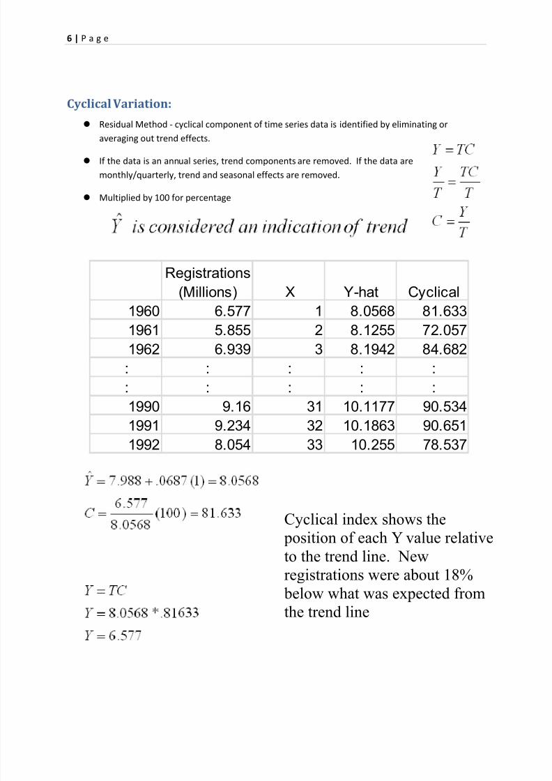
Residual Method - cyclical component of time series data is identified by eliminating or

averaging out trend effects.

If the data is an annual series, trend components are removed. If the data are

monthly/quarterly, trend and seasonal effects are removed.

Multiplied by 100 for percentage

Registrations(Millions) X Y-hat Cyclical

1960 6.577 1 8.0568 81.633

1961 5.855 2 8.1255 72.057

1962 6.939 3 8.1942 84.682

: : : : :

: : : : :

1990 9.16 31 10.1177 90.5341991 9.234 32 10.1863 90.651

1992 8.054 33 10.255 78.537

Cyclical index shows the

position of each Y value relative

to the trend line. New

registrations were about 18%

below what was expected from

the trend line



7 | P a g e

Plot the cyclical index over time

The trend line is the 100% base line.

Once plotted, it is very easy to see the cyclical patterns.

Does the series cycle?

If so, how extreme is the cycle?

Does the series follow the general economy/business cycle? (Do peaks occur when the

economy is strong and bottom out when the economy is weak?

Business indicator - business related time series that are used to help assess the general state of

the economy.

Economic Indicators:

Certain statistical time series may be useful as direct indicators of cyclical expansions and

contractions in business activity.

National Bureau of Economic Research has 22 business indicators:

Leading - anticipate turning points up or down

Coincident - indicate economy’s current performance

Lagging - lag behind the general upswing/downswing of the economy.

Cyclical Cautions:

Difficult to identify cyclical turning points near the time they occur - because the series also

contains short term irregular components

No uniformity occurs in the length of time by which a given leading indicator precedes cyclical

turns in the economy. For example, leading indicators may signal a recession or recovery some

time in the future, but they provide less help in establishing the timing of the turn.

False signals - a turning point does not materialize.

Should be used together with other data - but analysts should beware of limitations.



8 | P a g e

Long Term Forecasts:

Most important aspect is to predict the direction!

If the trend is the dynamic value, the model can be used to forecast long term. This isdetermined if the trend equation does a good job at fitting past data. If the cyclical is the most

important, the model should only be used to forecast one period ahead.

The equation estimates T and we use subjective data to estimate the cyclical effect for

Y-hat = T x C

7.988 + .0687(34) = 10.324 (this is the value for T)

Based on coincident and leading indicators, estimate an upswing. C is estimated to be 83.

Forecast for period 34 = 10.324*.83 = 8.569

Cyclical and Irregular Effects:

CI = Y/TS

I = CI/C

The irregular component measures the variability of the time series after the other components

have been removed.

Outboard Sales Example: (key the data on Page 04)

Use a combination of Minitab and Excel for the data analysis.

Outboard Sales Example:

T column is based on time series regression. Calculate the fitted values for each period

SCI column is Y/T

S column is from Minitab output - seasonal index per period

TCI column is Y/S

CI column is Y/TS

C column is a 3 month moving average of CI. This is the cyclical index for every quarter

I column is CI/C

Need to use Excel to calculate CI, C, and I



9 | P a g e

Seasonal Forecasting:

Forecast for trend with the equation

Use the adjusted seasonal index for the appropriate month/quarter

Estimate the cyclical component using indicators - remember the important aspect is to get thedirection correct

Commonly use 1 to indicate the irregular component since irregular effects are usually random

noise

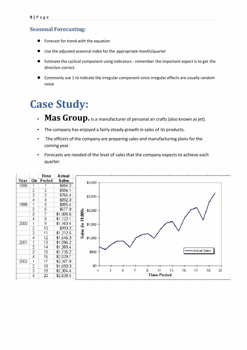
Case Study:• Mas Group. Is a manufacturer of personal air crafts (also known as jet).

• The company has enjoyed a fairly steady growth in sales of its products.

• The officers of the company are preparing sales and manufacturing plans for the

coming year.

• Forecasts are needed of the level of sales that the company expects to achieve each

quarter.



10 | P a g e

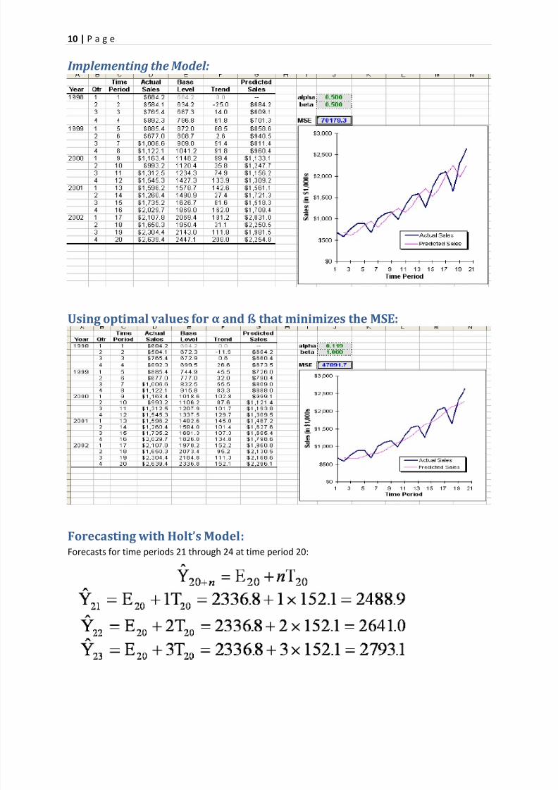
Implementing the Model:

Using optimal values for α and ß that minimizes the MSE:

Forecasting with Holt’s Model:

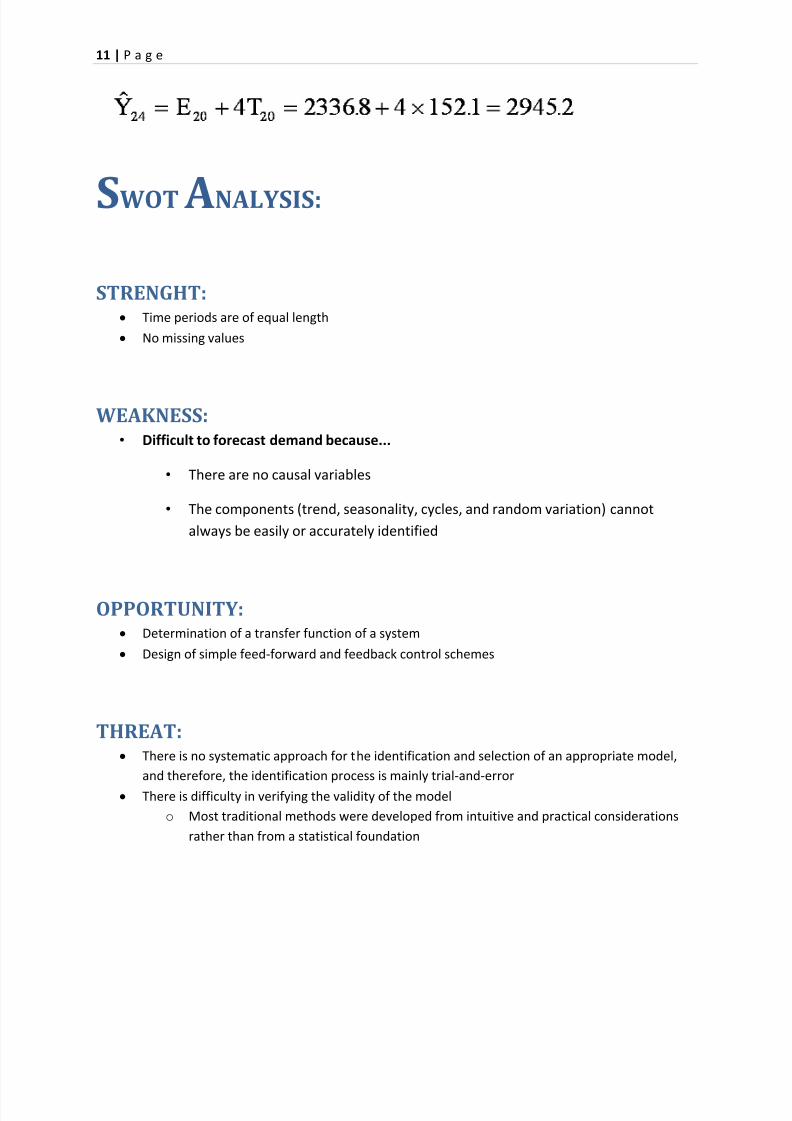
Forecasts for time periods 21 through 24 at time period 20:



11 | P a g e

SWOT ANALYSIS:

STRENGHT: Time periods are of equal length

No missing values

WEAKNESS:• Difficult to forecast demand because...

• There are no causal variables

• The components (trend, seasonality, cycles, and random variation) cannot

always be easily or accurately identified

OPPORTUNITY: Determination of a transfer function of a system

Design of simple feed-forward and feedback control schemes

THREAT: There is no systematic approach for the identification and selection of an appropriate model,

and therefore, the identification process is mainly trial-and-error

There is difficulty in verifying the validity of the model

o Most traditional methods were developed from intuitive and practical considerations

rather than from a statistical foundation



12 | P a g e

Conclusion:• Described what forecasting is

• Explained time series & its components

• Smoothed a data series

– Moving average

– Exponential smoothing

• Forecasted using trend models

Recommendation:

• Select several forecasting methods

• ‘Forecast’ the past

• Evaluate forecasts

•

Select best method

• Forecast the future

• Monitor continuously forecast accuracy

523 Assignement (Completed) Assg # 02

Documents

Transcript of 523 Assignement (Completed) Assg # 02