04/18/23 Chapter 3 1

Chapter 3

The Normal Distributions

04/18/23 Chapter 3 2

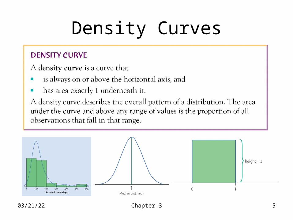
Density Curves• Here is a histogram

of vocabulary scores of n = 947 seventh graders

• The smooth curve drawn over the histogram is a mathematical model which represents the density function of the distribution

04/18/23 Chapter 3 3

Density Curves• The shaded bars on

this histogram corresponds to the scores that are less than 6.0

• This area represents is 30.3% of the total area of the histogram and is equal to the percentage in that range

04/18/23 Chapter 3 4

Area Under the Curve (AUC)

• This figure shades area under the curve (AUC) corresponding to scores less than 6

• This also corresponds to the proportion in that range: AUC = proportion in that range

04/18/23 Chapter 3 5

Density Curves

04/18/23 Chapter 3 6

Mean and Median of Density Curve

04/18/23 Chapter 3 7

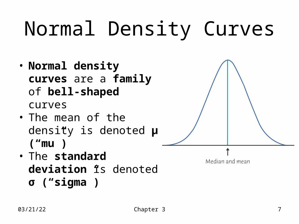
Normal Density Curves

• Normal density curves are a family of bell-shaped curves

• The mean of the density is denoted μ (“mu”)

• The standard deviation is denoted σ (“sigma”)

04/18/23 Chapter 3 8

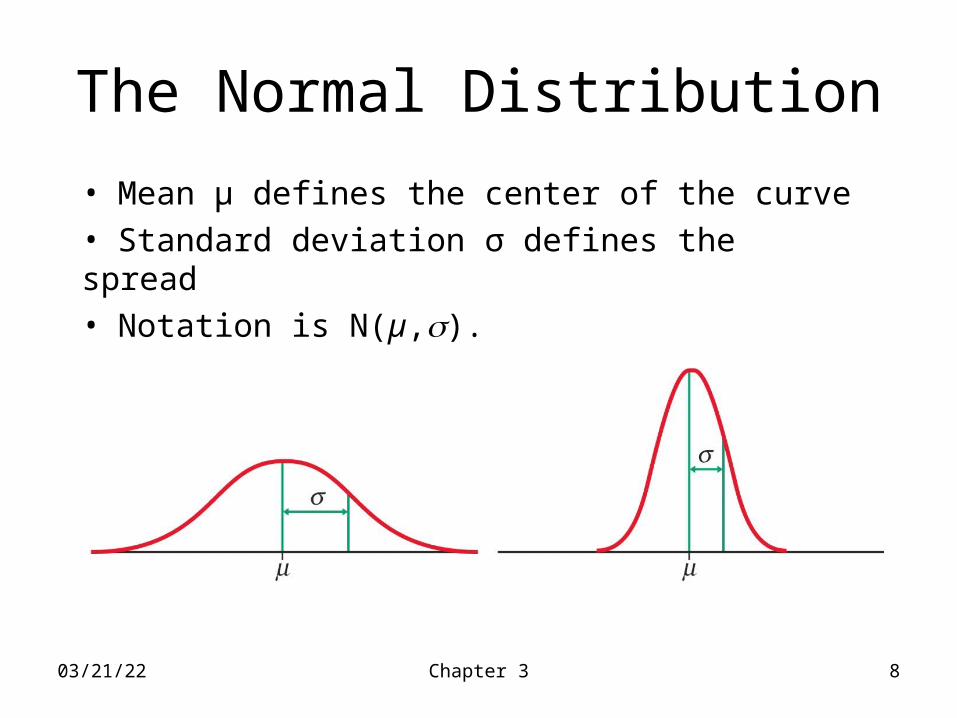
The Normal Distribution

• Mean μ defines the center of the curve• Standard deviation σ defines the spread• Notation is N(µ,).

04/18/23 Chapter 3 9

Practice Drawing Curves!

• The Normal curve is symmetrical around μ • It has infections (blue arrows) at μ ± σ

04/18/23 Chapter 3 10

The 68-95-99.7 Rule

• 68% of AUC within μ ± 1σ• 95% fall within μ ± 2σ• 99.7% within μ ± 3σ• Memorize!

This rule applies only to Normal curves

04/18/23 Chapter 3 11

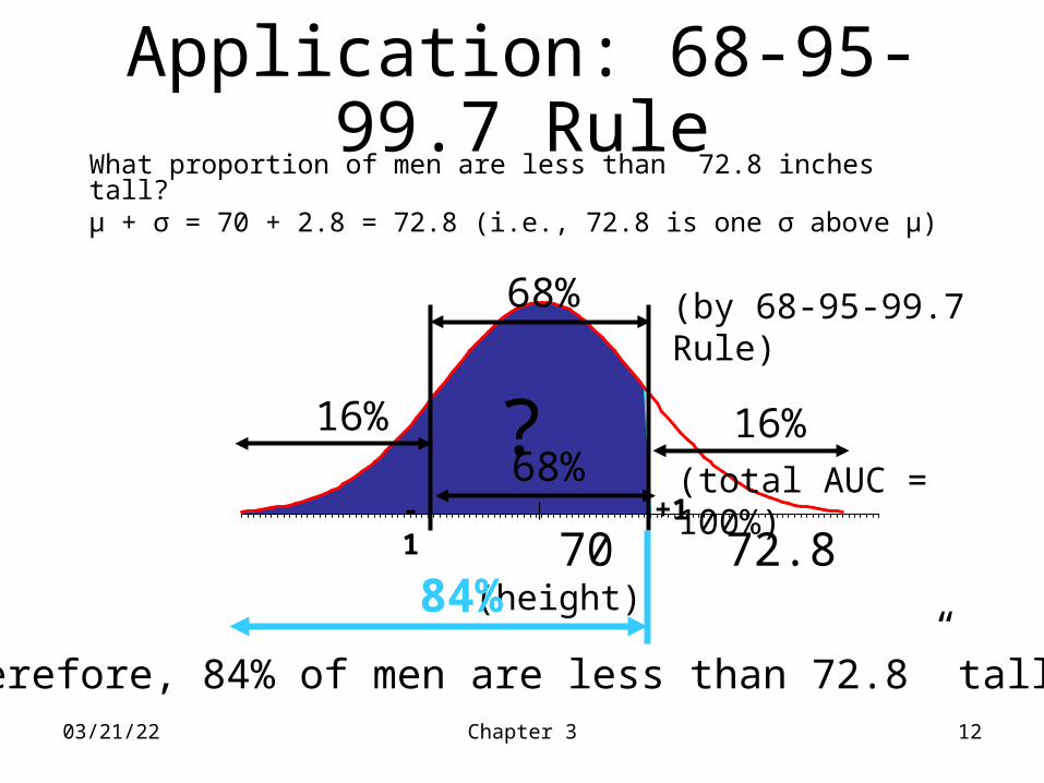
Application of 68-95-99.7 rule• Male height has a Normal distribution with μ = 70.0

inches and σ = 2.8 inches

• Notation: Let X ≡ male height; X~ N(μ = 70, σ = 2.8)

68-95-99.7 rule

• 68% in µ = 70.0 2.8 = 67.2 to 72.8

• 95% in µ 2 = 70.0 2(2.8) = 64.4 to 75.6

• 99.7% in µ 3 = 70.0 3(2.8) = 61.6 to 78.4

04/18/23 Chapter 3 12

Application: 68-95-99.7 RuleWhat proportion of men are less than 72.8 inches tall?μ + σ = 70 + 2.8 = 72.8 (i.e., 72.8 is one σ above μ)

?

70 72.8 (height) +1

84%

68% (by 68-95-99.7 Rule)

16%

-1

Therefore, 84% of men are less than 72.8” tall.

16%68% (total AUC = 100%)

04/18/23 Chapter 3 13

Finding Normal proportionsWhat proportion of men are less than 68” tall? This is equal to the AUC to the left of 68 on X~N(70,2.8)

?

68 70 (height values)

To answer this question, first determine the z-score for a value of 68 from X~N(70,2.8)

04/18/23 Chapter 3 14

Z score

• The z-score tells you how many standard deviation the value falls below (negative z score) or above (positive z score) mean μ

• The z-score of 68 when X~N(70,2.8) is:

71.08.2

7068

x

z

zx

Thus, 68 is 0.71 standard deviations below μ.

04/18/23 Chapter 3 15

Example: z score and associate value

-0.71 0 (z values)68 70 (height values)

?

04/18/23 Chapter 3 16

Standard Normal TableUse Table A to determine the cumulative proportion associated with the z score

See pp. 79 – 83 in your text!

04/18/23 Chapter 3 17

Normal Cumulative Proportions (Table A)

z .00 .02

0.8 .2119 .2090 .2061

.2420 .2358

0.6 .2743 .2709 .2676

0.7

.01

.2389

Thus, a z score of −0.71 has a cumulative proportion of .2389

04/18/23 Chapter 3 18

-0.71 0 (z scores)68 70 (height values)

Normal proportions

.2389

The proportion of mean less than 68” tall (z-score = −0.71 is .2389:

04/18/23 Chapter 3 19

Area to the right (“greater than”)

.2389

-0.71 0 (z values)68 70 (height values)

1.2389 = .7611

Since the total AUC = 1:AUC to the right = 1 – AUC to leftExample: What % of men are greater than 68” tall?

04/18/23 Chapter 3 20

Normal proportions“The key to calculating Normal proportions is to match the area you want with the areas that represent cumulative proportions. If you make a sketch of the area you want, you will almost never go wrong. Find areas for cumulative proportions … from [Table A] (p. 79)”

Follow the “method in the picture” (see pp. 79 – 80) to determine areas in right tails and between two points

04/18/23 Chapter 3 21

We just covered finding proportions for Normal variables. At other times, we may know the proportion and need to find the Normal value.

Method for finding a Normal value:1. State the problem 2. Sketch the curve3. Use Table A to look up the proportion & z-score4. Unstandardize the z-score with this formula

Finding Normal values

zx

04/18/23 Chapter 3 22

State the Problem & Sketch Curve

.10 ? 70 (height)

Problem: How tall must a man be to be taller than 10% of men in the population? (This is the same as asking how tall he has to be to be shorter than 90% of men.)

Recall X~N(70, 2.8)

04/18/23 Chapter 3 23

Table AFind z score for cumulative proportion ≈.10

z .07 .09

1.3 .0853 .0838 .0823

.1020 .0985

1.1 .1210 .1190 .1170

1.2

.08

.1003

zcum_proportion = z.1003 = −1.28

04/18/23 Chapter 3 24

Visual Relationship Between Cumulative proportion and z-score

-1.28 0 (Z value)

.10 ? 70 (height values)

04/18/23 Chapter 3 25

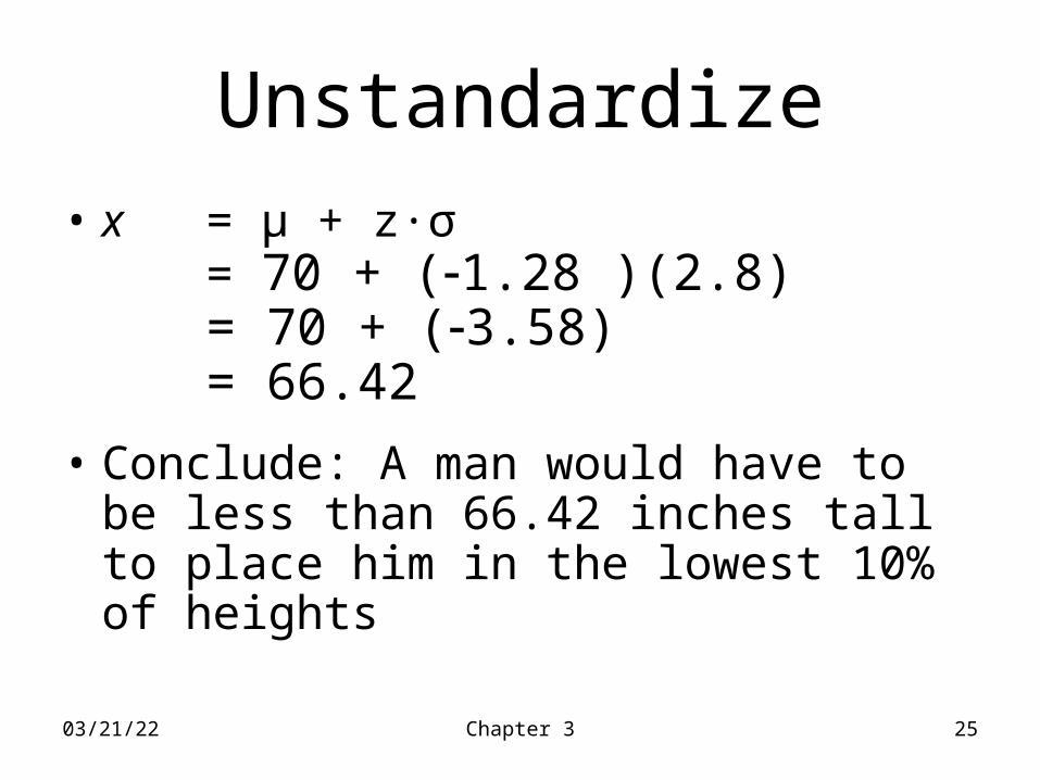
Unstandardize• x = μ + z∙σ

= 70 + (1.28 )(2.8) = 70 + (3.58) = 66.42

• Conclude: A man would have to be less than 66.42 inches tall to place him in the lowest 10% of heights