5.1 Externality Theory to Negative Externalities ... · PDF fileExternalities: Problems and...

In December 1997, representatives from over 170 nations met in Kyoto,Japan, to attempt one of the most ambitious international negotiationsever: an international pact to limit the emissions of carbon dioxide world-

wide. The motivation for this international gathering was increasing concernover the problem of global warming. As Figure 5-1 on p. 122 shows, there hasbeen a steady rise in global temperatures over the twentieth century. A grow-ing scientific consensus suggests that the cause of this warming trend is humanactivity, in particular the use of fossil fuels. The burning of fossil fuels such ascoal, oil, natural gas, and gasoline produces carbon dioxide, which in turn trapsthe heat from the sun in the earth’s atmosphere. Many scientists predict that,over the next century, global temperatures could rise by as much as tendegrees Fahrenheit.1

If you are reading this in North Dakota, that may sound like good news.Indeed, for much of the United States, this increase in temperatures willimprove agricultural output as well as quality of life. In most areas around theworld, however, the impacts of global warming would be unwelcome, and inmany cases, disastrous. The global sea level could rise by almost three feet,increasing risks of flooding and submersion of low - lying coastal areas. Somescientists project, for example, that 20–40% of the entire country ofBangladesh will be flooded due to global warming over the next century, withmuch of this nation being under more than five feet of water!2

Despite this dire forecast, the nations gathered in Kyoto faced a dauntingtask. The cost of reducing the use of fossil fuels, particularly in the majorindustrialized nations, is enormous. Fossil fuels are central to heating ourhomes, transporting us to our jobs, and lighting our places of work. Replacingthese fossil fuels with alternatives would significantly raise the costs of living in

Externalities: Problems and Solutions

5

121

5.1 Externality Theory

5.2 Private - Sector Solutionsto Negative Externalities

5.3 Public - Sector Remediesfor Externalities

5.4 Distinctions BetweenPrice and Quantity Approachesto Addressing Externalities

5.5 Conclusion

1 International Panel on Climate Change (2001). Global warming is produced not just by carbon dioxidebut by other gases, such as methane, as well, but carbon dioxide is the main cause and for ease we use carbondioxide as shorthand for the full set of “greenhouse gases.”2 Mirza et al. (2003).

Gru3e_Ch05.qxp:Gru3e_Ch05 11/17/09 2:04 PM 21

developed countries. To end the problem of global warming, some predict thatwe will have to reduce our use of fossil fuels to nineteenth - century (pre - industrial) levels. Yet, even to reduce fossil fuel use to the level ultimately man-dated by this Kyoto conference (7% below 1990 levels) could cost the UnitedStates $1.1 trillion, or about 10% of GDP.3 Thus, it is perhaps not surprisingthat the United States has yet to ratify the treaty agreed to at Kyoto.

Global warming due to emissions of fossil fuels is a classic example of whateconomists call an externality. An externality occurs whenever the actions ofone party make another party worse or better off, yet the first party neitherbears the costs nor receives the benefits of doing so. Thus, when we drive carsin the United States we increase emissions of carbon dioxide, raise world tem-peratures, and thereby increase the likelihood that in 100 years Bangladeshwill be flooded out of existence. Did you know this when you drove to classtoday? Not unless you are a very interested student of environmental policy.Your enjoyment of your driving experience is in no way diminished by thedamage that your emissions are causing.

Externalities occur in many everyday interactions. Sometimes they arelocalized and small, such as the impact on your roommate if you play yourstereo too loudly or the impact on your neighbors if your dog uses their gardenas a bathroom. Externalities also exist on a much larger scale, such as globalwarming or acid rain. When utilities in the Midwest produce electricity usingcoal, a by - product of that production is the emission of sulfur dioxide andnitrogen oxides into the atmosphere, where they form sulfuric and nitric acids.

122 P A R T I I ■ E X T E R N A L I T I E S A N D P U B L I C G O O D S

Average Global Temperature, 1880 to 2008 • There was a steady upward trend in global temperatures throughout the twentieth century.

Source: Figure adapted from NASA’s Goddard Institute for Space Studies, “Global Annual Mean Surface Air Temperature Change,” located athttp://data.giss.nasa.gov/gistemp/graphs/Fig.A2.lrg.gif

Global averagetemperature(degrees F)

2000 2010199019801970193019201910190018901880 196019501940

58.5

58

57.5

57

56.5

56

■ FIGURE 5-1

3 This is the total cost over future years of reducing emissions, not a one-year cost. Nordhaus and Boyer(2000), Table 8.6 (updated to 2000 dollars).

externality Externalities arisewhenever the actions of oneparty make another party worseor better off, yet the first partyneither bears the costs norreceives the benefits of doingso.

Gru3e_Ch05.qxp:Gru3e_Ch05 11/17/09 2:04 PM Page 122

These acids may fall back to earth hundreds of miles away, in the processdestroying trees, causing billions of dollars of property damage, and increasingrespiratory problems in the population. Without government intervention, theutilities in the Midwest bear none of the cost for the polluting effects of theirproduction activities.

Externalities are a classic example of the type of market failures discussedin Chapter 1. Recall that the most important of our four questions of publicfinance is when is it appropriate for the government to intervene? As we willshow in this chapter, externalities present a classic justification for governmentintervention. Indeed, 168,974 federal employees, or about 5% of the federalworkforce, are ostensibly charged with dealing with environmental externali-ties in agencies such as the Environmental Protection Agency and the Depart-ment of the Interior.4

This chapter begins with a discussion of the nature of externalities. Wefocus primarily throughout the chapter on environmental externalities,although we briefly discuss other applications as well. We then ask whethergovernment intervention is necessary to combat externalities, and under whatconditions the private market may be able to solve the problem. We discuss theset of government tools available to address externalities, comparing their costsand benefits under various assumptions about the markets in which the gov-ernment is intervening. In the next chapter, we apply these theories to thestudy of some of the most important externality issues facing the UnitedStates and other nations today: acid rain, global warming, and smoking.

5.1Externality Theory

In this section, we develop the basic theory of externalities. As we emphasizenext, externalities can arise either from the production of goods or from

their consumption and can be negative (as in the examples discussed above) orpositive. We begin with the classic case of a negative production externality.

Economics of Negative Production ExternalitiesSomewhere in the United States there is a steel plant located next to a river.This plant produces steel products, but it also produces “sludge,” a by - productuseless to the plant owners. To get rid of this unwanted by - product, the own-ers build a pipe out the back of the plant and dump the sludge into the river.The sludge produced is directly proportional to the production of steel; eachadditional unit of steel creates one more unit of sludge as well.

The steel plant is not the only producer using the river, however. Fartherdownstream is a traditional fishing area where fishermen catch fish for sale to

C H A P T E R 5 ■ E X T E R N A L I T I E S : P R O B L E M S A N D S O L U T I O N S 123

market failure A problem thatcauses the market economy todeliver an outcome that doesnot maximize efficiency.

4 Estimates from U.S. Office of Personnel Management (2007), pg. 88.


local restaurants. Since the steel plant has begun dumping sludge into the river,the fishing has become much less profitable because there are many fewer fishleft alive to catch.

This scenario is a classic example of what we mean by an externality. Thesteel plant is exerting a negative production externality on the fishermen,since its production adversely affects the well - being of the fishermen but theplant does not compensate the fishermen for their loss.

One way to see this externality is to graph the market for the steel producedby this plant (Figure 5-2) and to compare the private benefits and costs of pro-duction to the social benefits and costs. Private benefits and costs are the benefitsand costs borne directly by the actors in the steel market (the producers andconsumers of the steel products). Social benefits and costs are the private benefitsand costs plus the benefits and costs to any actors outside this steel market whoare affected by the steel plant’s production process (the fishermen).

Recall from Chapter 2 that each point on the market supply curve for agood (steel, in our example) represents the market’s marginal cost of produc-ing that unit of the good—that is, the private marginal cost (PMC) of thatunit of steel. What determines the welfare consequences of production, how-ever, is the social marginal cost (SMC), which equals the private marginalcost to the producers of producing that next unit of a good plus any costs asso-ciated with the production of that good that are imposed on others. This distinctionwas not made in Chapter 2, because without market failures SMC � PMC, thesocial costs of producing steel are equal to the costs to steel producers. Thus,


negative production exter-nality When a firm’s productionreduces the well - being of otherswho are not compensated bythe firm.

private marginal cost (PMC)The direct cost to producers ofproducing an additional unit of agood.

social marginal cost (SMC)The private marginal cost toproducers plus any costs asso-ciated with the production of thegood that are imposed on others.

Market Failure Due to NegativeProduction Externalities in theSteel Market • A negative productionexternality of $100 per unit of steelproduced (marginal damage, MD) leadsto a social marginal cost that is abovethe private marginal cost, and a socialoptimum quantity (Q2) that is lowerthan the competitive market equilibriumquantity (Q1). There is overproductionof Q1 � Q2, with an associated dead-weight loss of area BCA.

■ FIGURE 5-2

P1

Quantity of steel

Price ofsteel

Q1Q2

D = Privatemarginal benefit,PMB = Socialmarginal benefit,SMB

S = Privatemarginal cost,PMC

$100 = Marginaldamage, MD

Deadweight loss

Social marginalcost, SMC=PMC+MD

A

B

C

Overproduction


when we computed social welfare in Chapter 2 we did so with reference tothe supply curve.

This approach is not correct in the presence of externalities, however.When there are externalities, SMC � PMC � MD, where MD is the margin-al damage done to others, such as the fishermen, from each unit of production(marginal because it is the damage associated with that particular unit of pro-duction, not total production). Suppose, for example, that each unit of steelproduction creates sludge that kills $100 worth of fish. In Figure 5-2, the SMCcurve is therefore the PMC (supply) curve, shifted upward by the marginaldamage of $100.5 That is, at Q1 units of production (point A), the social mar-ginal cost is the private marginal cost at that point (which is equal to P1), plus$100 (point B). For every level of production, social costs are $100 higher thanprivate costs, since each unit of production imposes $100 of costs on the fish-ermen for which they are not compensated.

Recall also from Chapter 2 that each point on the market demand curvefor steel represents the sum of individual willingnesses to pay for that unit ofsteel, or the private marginal benefit (PMB) of that unit of steel. Onceagain, however, the welfare consequences of consumption are defined relativeto the social marginal benefit (SMB), which equals the private marginalbenefit to the consumers minus any costs associated with the consumption of thegood that are imposed on others. In our example, there are no such costs imposedby the consumption of steel, so SMB � PMB in Figure 5-2.

In Chapter 2, we showed that the private market competitive equilibriumis at point A in Figure 5-2, with a level of production Q1 and a price of P1. Wealso showed that this was the social - efficiency - maximizing level of consump-tion for the private market. In the presence of externalities, this relationshipno longer holds true. Social efficiency is defined relative to social marginalbenefit and cost curves, not to private marginal benefit and cost curves.Because of the negative externality of sludge dumping, the social curves (SMBand SMC) intersect at point C, with a level of consumption Q2. Since thesteel plant owner doesn’t account for the fact that each unit of steel produc-tion kills fish downstream, the supply curve understates the costs of producingQ1 to be at point A, rather than at point B. As a result, too much steel is pro-duced (Q1 � Q2), and the private market equilibrium no longer maximizessocial efficiency.

When we move away from the social - efficiency - maximizing quantity, wecreate a deadweight loss for society because units are produced and consumedfor which the cost to society (summarized by curve SMC) exceeds the socialbenefits (summarized by curve D � SMB). In our example, the deadweightloss is equal to the area BCA. The width of the deadweight loss triangle isdetermined by the number of units for which social costs exceed social bene-fits (Q1 � Q2). The height of the triangle is the difference between the mar-ginal social cost and the marginal social benefit, the marginal damage.


private marginal benefit(PMB) The direct benefit toconsumers of consuming anadditional unit of a good by theconsumer.

social marginal benefit(SMB) The private marginalbenefit to consumers minus anycosts associated with the con-sumption of the good that areimposed on others.

5 This example assumes that the damage from each unit of steel production is constant, but in reality thedamage can rise or fall as production changes. Whether the damage changes or remains the same affects theshape of the social marginal cost curve, relative to the private marginal cost curve.


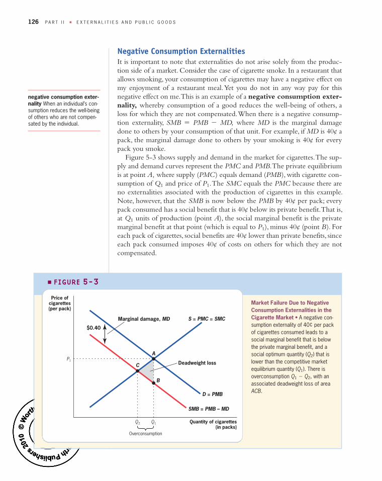
Negative Consumption ExternalitiesIt is important to note that externalities do not arise solely from the produc-tion side of a market. Consider the case of cigarette smoke. In a restaurant thatallows smoking, your consumption of cigarettes may have a negative effect onmy enjoyment of a restaurant meal. Yet you do not in any way pay for thisnegative effect on me. This is an example of a negative consumption exter-nality, whereby consumption of a good reduces the well - being of others, aloss for which they are not compensated. When there is a negative consump-tion externality, SMB � PMB � MD, where MD is the marginal damagedone to others by your consumption of that unit. For example, if MD is 40¢ apack, the marginal damage done to others by your smoking is 40¢ for everypack you smoke.

Figure 5-3 shows supply and demand in the market for cigarettes. The sup-ply and demand curves represent the PMC and PMB. The private equilibriumis at point A, where supply (PMC) equals demand (PMB), with cigarette con-sumption of Q1 and price of P1. The SMC equals the PMC because there areno externalities associated with the production of cigarettes in this example.Note, however, that the SMB is now below the PMB by 40¢ per pack; everypack consumed has a social benefit that is 40¢ below its private benefit. That is,at Q1 units of production (point A), the social marginal benefit is the privatemarginal benefit at that point (which is equal to P1), minus 40¢ (point B). Foreach pack of cigarettes, social benefits are 40¢ lower than private benefits, sinceeach pack consumed imposes 40¢ of costs on others for which they are notcompensated.


negative consumption exter-nality When an individual’s con-sumption reduces the well - beingof others who are not compen-sated by the individual.

Market Failure Due to NegativeConsumption Externalities in theCigarette Market • A negative con-sumption externality of 40¢ per packof cigarettes consumed leads to asocial marginal benefit that is belowthe private marginal benefit, and asocial optimum quantity (Q2) that islower than the competitive marketequilibrium quantity (Q1). There isoverconsumption Q1 � Q2, with anassociated deadweight loss of areaACB.

■ FIGURE 5-3

P1

Quantity of cigarettes(in packs)

Price ofcigarettes(per pack)

Q1Q2

Overconsumption

D = PMB

S = PMC = SMCMarginal damage, MD

A

C

B

$0.40

SMB = PMB – MD

Deadweight loss


The social - welfare - maximizing level of consumption, Q2, is identified bypoint C, the point at which SMB � SMC. There is overconsumption of ciga-rettes by Q1 � Q2: the social costs (point A on the SMC curve) exceed socialbenefits (on the SMB curve) for all units between Q1 and Q2. As a result, thereis a deadweight loss (area ACB) in the market for cigarettes.

�

The Externality of SUVs6

In 1985, the typical driver sat behind the wheel of a car that weighed about3,200 pounds, and the largest cars on the road weighed 4,600 pounds. In2008, the typical driver is in a car that weighted about 4,117 pounds andthe largest cars on the road can weigh 8,500 pounds. The major culprits inthis evolution of car size are sport utility vehicles (SUVs). The term SUVwas originally reserved for large vehicles intended for off - road driving,but it now refers to any large passenger vehicle marketed as an SUV, even ifit lacks off - road capabilities. SUVs, with an average weight of 4,742 pounds,represented only 6.4% of vehicle sales as recently as 1988, but 20 yearslater, in 2008, they accounted for over 29.6% of the new vehicles soldeach year.

The consumption of large cars such as SUVs produces three types of nega-tive externalities:

Environmental Externalities The contribution of driving to global warm-ing is directly proportional to the amount of fossil fuel a vehicle requires totravel a mile. The typical compact or mid - size car gets roughly 25 miles to thegallon but the typical SUV gets only 20 miles per gallon. This means that SUVdrivers use more gas to go to work or run their errands, increasing fossil fuelemissions. This increased environmental cost is not paid by those who driveSUVs.

Wear and Tear on Roads Each year, federal, state, and local governments inthe United States spend $33.1 billion repairing our roadways. Damage toroadways comes from many sources, but a major culprit is the passenger vehi-cle, and the damage it does to the roads is proportional to vehicle weight.When individuals drive SUVs, they increase the cost to government ofrepairing the roads. SUV drivers bear some of these costs through gasolinetaxes (which fund highway repair), since the SUV uses more gas, but it isunclear if these extra taxes are enough to compensate for the extra damagedone to roads.

APPLICATION


6 All data in this application are from the U.S. Environmental Protection Agency (2008) and the U.S.Department of Transportation (2009).


Safety Externalities One major appeal of SUVs is that they provide a feelingof security because they are so much larger than other cars on the road. Off-setting this feeling of security is the added insecurity imposed on other cars onthe road. For a car of average weight, the odds of having a fatal accident rise byfour times if the accident is with a typical SUV and not with a car of the samesize. Thus, SUV drivers impose a negative externality on other drivers becausethey don’t compensate those other drivers for the increased risk of a danger-ous accident. �

Positive ExternalitiesWhen economists think about externalities, they tend to focus on negativeexternalities, but not all externalities are bad. There may also be positive pro-duction externalities associated with a market, whereby production benefitsparties other than the producer and yet the producer is not compensated.Imagine the following scenario: There is public land beneath which theremight be valuable oil reserves. The government allows any oil developer to drillin those public lands, as long as the government gets some royalties on any oilreserves found. Each dollar the oil developer spends on exploration increasesthe chances of finding oil reserves. Once found, however, the oil reserves canbe tapped by other companies; the initial driller only has the advantage of get-ting there first. Thus, exploration for oil by one company exerts a positive pro-duction externality on other companies: each dollar spent on exploration by thefirst company raises the chance that other companies will have a chance tomake money from new oil found on this land.

Figure 5-4 shows the market for oil exploration to illustrate the positiveexternality to exploration: the social marginal cost of exploration is actuallylower than the private marginal cost because exploration has a positive effecton the future profits of other companies. Assume that the marginal benefit ofeach dollar of exploration by one company, in terms of raising the expectedprofits of other companies who drill the same land, is a constant amount MB.As a result, the SMC is below the PMC by the amount MB. Thus, the privateequilibrium in the exploration market (point A, quantity Q1) leads to under-production relative to the socially optimal level (point B, quantity Q2) becausethe initial oil company is not compensated for the benefits it confers on otheroil producers.

Note also that there can be positive consumption externalities. Imag-ine, for example, that my neighbor is considering improving the landscapingaround his house. The improved landscaping will cost him $1,000, but it isonly worth $800 to him. My bedroom faces his house, and I would like tohave nicer landscaping to look at. This better view would be worth $300 tome. That is, the total social marginal benefit of the improved landscaping is$1,100, even though the private marginal benefit to my neighbor is only $800.Since this social marginal benefit ($1,100) is larger than the social marginalcosts ($1,000), it would be socially efficient for my neighbor to do the land-scaping. My neighbor won’t do the landscaping, however, since his private


positive production external-ity When a firm’s productionincreases the well - being of others but the firm is not com-pensated by those others.

positive consumption exter-nality When an individual’s consumption increases the well - being of others but the individ-ual is not compensated bythose others.


Qcosts ($1,000) exceed his private benefits. His landscaping improvementswould have a positive effect on me for which he will not be compensated,thus leading to an underconsumption of landscaping.

Quick Hint One confusing aspect of the graphical analysis of externalitiesis knowing which curve to shift, and in which direction. To review, there are fourpossibilities:� Negative production externality: SMC curve lies above PMC curve.� Positive production externality: SMC curve lies below PMC curve.� Negative consumption externality: SMB curve lies below PMB curve.� Positive consumption externality: SMB curve lies above PMB curve.

Armed with these facts, the key is to assess which category a particular example

fits into. This assessment is done in two steps. First, you must assess whether

the externality is associated with producing a good or with consuming a good.

Then, you must assess whether the externality is positive or negative.

The steel plant example is a negative production externality because the

externality is associated with the production of steel, not its consumption; the

sludge doesn’t come from using steel, but rather from making it. Likewise, our

cigarette example is a negative consumption externality because the externality

is associated with the consumption of cigarettes; secondhand smoke doesn’t

come from making cigarettes, it comes from smoking them.


Market Failure Due to PositiveProduction Externality in the OilExploration Market • Expendi-tures on oil exploration by any com-pany have a positive externalitybecause they offer more profitableopportunities for other companies.This leads to a social marginal costthat is below the private marginalcost, and a social optimum quantity(Q2) that is greater than the com-petitive market equilibrium quantity(Q1). There is underproduction of Q2 � Q1, with an associateddeadweight loss of area ABC.

■ FIGURE 5-4

P1

Quantity of oilexploration

Price ofoil exploration

Q1 Q2

P2

Underproduction

Deadweight loss

Marginalbenefit,MB

S = PMC

D = PMB = SMB

A

C

B

SMC = PMC – MB


5.2Private-Sector Solutions to Negative Externalities

In microeconomics, the market is innocent until proven guilty (and, similar-ly, the government is often guilty until proven innocent!). An excellent

application of this principle can be found in a classic work by Ronald Coase,a professor at the Law School at the University of Chicago, who asked in1960: Why won’t the market simply compensate the affected parties forexternalities?7

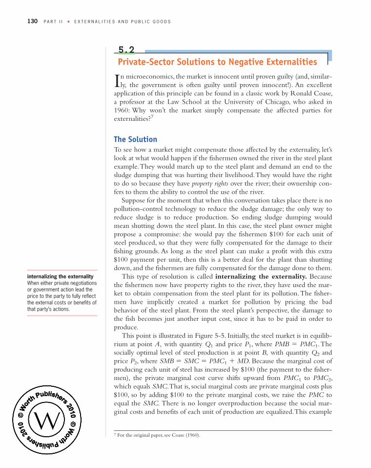
The SolutionTo see how a market might compensate those affected by the externality, let’slook at what would happen if the fishermen owned the river in the steel plantexample. They would march up to the steel plant and demand an end to thesludge dumping that was hurting their livelihood. They would have the rightto do so because they have property rights over the river; their ownership con-fers to them the ability to control the use of the river.

Suppose for the moment that when this conversation takes place there is nopollution - control technology to reduce the sludge damage; the only way toreduce sludge is to reduce production. So ending sludge dumping wouldmean shutting down the steel plant. In this case, the steel plant owner mightpropose a compromise: she would pay the fishermen $100 for each unit ofsteel produced, so that they were fully compensated for the damage to theirfishing grounds. As long as the steel plant can make a profit with this extra$100 payment per unit, then this is a better deal for the plant than shuttingdown, and the fishermen are fully compensated for the damage done to them.

This type of resolution is called internalizing the externality. Becausethe fishermen now have property rights to the river, they have used the mar-ket to obtain compensation from the steel plant for its pollution. The fisher-men have implicitly created a market for pollution by pricing the badbehavior of the steel plant. From the steel plant’s perspective, the damage tothe fish becomes just another input cost, since it has to be paid in order toproduce.

This point is illustrated in Figure 5-5. Initially, the steel market is in equilib-rium at point A, with quantity Q1 and price P1, where PMB � PMC1. Thesocially optimal level of steel production is at point B, with quantity Q2 andprice P2, where SMB � SMC � PMC1 � MD. Because the marginal cost ofproducing each unit of steel has increased by $100 (the payment to the fisher-men), the private marginal cost curve shifts upward from PMC1 to PMC2,which equals SMC. That is, social marginal costs are private marginal costs plus$100, so by adding $100 to the private marginal costs, we raise the PMC toequal the SMC. There is no longer overproduction because the social mar-ginal costs and benefits of each unit of production are equalized. This example


7 For the original paper, see Coase (1960).

internalizing the externalityWhen either private negotiationsor government action lead theprice to the party to fully reflectthe external costs or benefits ofthat party’s actions.


illustrates Part I of the Coase Theorem: when there are well - defined prop-erty rights and costless bargaining, then negotiations between the party creat-ing the externality and the party affected by the externality can bring about thesocially optimal market quantity. This theorem states that externalities do notnecessarily create market failures, because negotiations between the parties canlead the offending producers (or consumers) to internalize the externality, oraccount for the external effects in their production (or consumption).

The Coase theorem suggests a very particular and limited role for the gov-ernment in dealing with externalities: establishing property rights. In Coase’sview, the fundamental limitation to implementing private - sector solutions toexternalities is poorly established property rights. If the government can estab-lish and enforce those property rights, then the private market will do the rest.

The Coase theorem also has an important Part II: the efficient solution toan externality does not depend on which party is assigned the property rights,as long as someone is assigned those rights. We can illustrate the intuitionbehind Part II using the steel plant example. Suppose that the steel plant,rather than the fishermen, owned the river. In this case, the fishermen wouldhave no right to make the plant owner pay a $100 compensation fee for eachunit of steel produced. The fishermen, however, would find it in their interestto pay the steel plant to produce less. If the fishermen promised the steel plantowner a payment of $100 for each unit he did not produce, then the steelplant owner would rationally consider there to be an extra $100 cost to eachunit he did produce. Remember that in economics, opportunity costs areincluded in a firm’s calculation of costs; thus, forgoing a payment from thefishermen of $100 for each unit of steel not produced has the same effect on


A Coasian Solution to NegativeProduction Externalities in theSteel Market • If the fishermencharge the steel plant $100 per unitof steel produced, this increases theplant’s private marginal cost curvefrom PMC1 to PMC2, which coincideswith the SMC curve. The quantity pro-duced falls from Q1 to Q2, the sociallyoptimal level of production. Thecharge internalizes the externality andremoves the inefficiency of the nega-tive externality.

■ FIGURE 5-5

P1

Quantity of steel

Price ofsteel

Q1Q2

D = PMB = SMBMD =$100

Payment

SMC = PMC2

S = PMC1

A

BP2

Coase Theorem (Part I) Whenthere are well - defined propertyrights and costless bargaining,then negotiations between theparty creating the externalityand the party affected by theexternality can bring about thesocially optimal market quantity.

Coase Theorem (Part II) Theefficient solution to an externalitydoes not depend on which partyis assigned the property rights,as long as someone is assignedthose rights.


Qproduction decisions as being forced to pay $100 extra for each unit of steelproduced. Once again, the private marginal cost curve would incorporate thisextra (opportunity) cost and shift out to the social marginal cost curve, andthere would no longer be overproduction of steel.

Quick Hint You may wonder why the fishermen would ever engage in either

of these transactions: they receive $100 for each $100 of damage to fish, or pay

$100 for each $100 reduction in damage to fish. So what is in it for them?

The answer is that this is a convenient shorthand economics modelers use for

saying, “The fishermen would charge at least $100 for sludge dumping” or “The

fishermen would pay up to $100 to remove sludge dumping.” By assuming that

the payments are exactly $100, we can conveniently model private and social

marginal costs as equal. It may be useful for you to think of the payment to the

fishermen as $101 and the payment from the fishermen as $99, so that the fish-

ermen make some money and private and social costs are approximately equal.

In reality, the payments to or from the fishermen will depend on the negotiating

power and skill of both parties in this transaction, highlighting the importance

of the issues raised next.

The Problems with Coasian SolutionsThis elegant theory would appear to rescue the standard competitive modelfrom this important cause of market failures and make government interven-tion unnecessary (other than to ensure property rights). In practice, however,the Coase theorem is unlikely to solve many of the types of externalities thatcause market failures. We can see this by considering realistically the problemsinvolved in achieving a “Coasian solution” to the problem of river pollution.

The Assignment Problem The first problem involves assigning blame. Riverscan be very long, and there may be other pollution sources along the way thatare doing some of the damage to the fish. The fish may also be dwindling fornatural reasons, such as disease or a rise in natural predators. In many cases, it isimpossible to assign blame for externalities to one specific entity.

Assigning damage is another side to the assignment problem. We haveassumed that the damage was a fixed dollar amount, $100. Where does this fig-ure come from in practice? Can we trust the fishermen to tell us the rightamount of damage that they suffer? It would be in their interest in anyCoasian negotiation to overstate the damage in order to ensure the largestpossible payment. And how will the payment be distributed among the fisher-men? When a number of individuals are fishing the same area, it is difficult tosay whose catch is most affected by the reduction in the stock of available fish.

The significance of the assignment problem as a barrier to internalizing theexternality depends on the nature of the externality. If my loud stereo playingdisturbs your studying, then assignment of blame and damages is clear. In thecase of global warming, however, how can we assign blame clearly when carbon



emissions from any source in the world contribute to this problem? And howcan we assign damages clearly when some individuals would like the world tobe hotter, while others would not? Because of assignment problems, Coasiansolutions are likely to be more effective for small, localized externalities than forlarger, more global externalities.

The Holdout Problem Imagine that we have surmounted the assignmentproblem and that by careful scientific analysis we have determined that eachunit of sludge from the steel plant kills $1 worth of fish for each of 100 fisher-men, for a total damage of $100 per unit of steel produced.

Now, suppose that the fishermen have property rights to the river, and thesteel plant can’t produce unless all 100 fishermen say it can. The Coasian solu-tion is that each of the 100 fishermen gets paid $1 per unit of steel production,and the plant continues to produce steel. Each fisherman walks up to the plantand collects his check for $1 per unit. As the last fisherman is walking up, herealizes that he suddenly has been imbued with incredible power: the steelplant cannot produce without his permission since he is a part owner of theriver. So, why should he settle for only $1 per unit? Having already paid out$99 per unit, the steel plant would probably be willing to pay more than$1 per unit to remove this last obstacle to their production. Why not ask for$2 per unit? Or even more?

This is an illustration of the holdout problem, which can arise when theproperty rights in question are held by more than one party: the shared prop-erty rights give each owner power over all others. If the other fishermen arethinking ahead they will realize this might be a problem, and they will all tryto be the last one to go to the plant. The result could very well be a break-down of the negotiations and an inability to negotiate a Coasian solution. Aswith the assignment problem, the holdout problem would be amplified with ahuge externality like global warming, where billions of persons are potentiallydamaged.

The Free Rider Problem Can we solve the holdout problem by simplyassigning the property rights to the side with only one negotiator, in this casethe steel plant? Unfortunately, doing so creates a new problem.

Suppose that the steel plant has property rights to the river, and it agrees toreduce production by 1 unit for each $100 received from fishermen. Then theCoasian solution would be for the fishermen to pay $100, and for the plant tothen move to the optimal level of production. Suppose that the optimalreduction in steel production (where social marginal benefits and costs areequal) is 100 units, so that each fisherman pays $100 for a total of $10,000, andthe plant reduces production by 100 units.

Suppose, once again, that you are the last fisherman to pay. The plant hasalready received $9,900 to reduce its production, and will reduce its produc-tion as a result by 99 units. The 99 units will benefit all fishermen equally sincethey all share the river. Thus, as a result, if you don’t pay your $100, you willstill be almost as well off in terms of fishing as if you do. That is, the damageavoided by that last unit of reduction will be shared equally among all 100


holdout problem Shared own-ership of property rights giveseach owner power over all theothers.

Gru3e_Ch05.qxp:Gru3e_Ch05 11/17/09 2:05 PM 3

fishermen who use the river, yet you will pay the full $100 to buy that last unitof reduction. Thought of that way, why would you pay? This is an example ofthe free rider problem: when an investment has a personal cost but a com-mon benefit, individuals will underinvest. Understanding this incentive, yourfellow fishermen will also not pay their $100, and the externality will remainunsolved; if the other fishermen realize that someone is going to grab a freeride, they have little incentive to pay in the first place.

Transaction Costs and Negotiating Problems Finally, the Coasian approachignores the fundamental problem that it is hard to negotiate when there arelarge numbers of individuals on one or both sides of the negotiation. How canthe 100 fishermen effectively get together and figure out how much to chargeor pay the steel plant? This problem is amplified for an externality such asglobal warming, where the potentially divergent interests of billions of partieson one side must be somehow aggregated for a negotiation.

Moreover, these problems can be significant even for the small - scale, local-ized externalities for which Coase’s theory seems best designed. In theory, myneighbor and I can work out an appropriate compensation for my loud musicdisturbing his studying. In practice, this may be a socially awkward conversa-tion that is more likely to result in tension than in a financial payment. Simi-larly, if the person next to me in the restaurant is smoking, it would be faroutside the norm, and probably considered insulting, to lean over and offerhim $5 to stop smoking. Alas, the world does not always operate in the rationalway economists wish it would!

Bottom Line Ronald Coase’s insight that externalities can sometimes beinternalized was a brilliant one. It provides the competitive market model witha defense against the onslaught of market failures that we will bring to bear onit throughout this course. It is also an excellent reason to suspect that the mar-ket may be able to internalize some small - scale, localized externalities. Where itwon’t help, as we’ve seen, is with large - scale, global externalities that are thefocus of, for example, environmental policy in the United States. The govern-ment may therefore have a role to play in addressing larger externalities.

5.3Public-Sector Remedies for Externalities

In the United States, public policy makers do not think that Coasian solu-tions are sufficient to deal with large - scale externalities. The Environmental

Protection Agency (EPA) was formed in 1970 to provide public - sector solu-tions to the problems of externalities in the environment. The agency regulatesa wide variety of environmental issues, in areas ranging from clean air to cleanwater to land management.8


free rider problem When aninvestment has a personalcost but a common benefit, individuals will underinvest.

8 See http://www.epa.gov/epahome/aboutepa.htm for more information. There are government resourcesdevoted to environmental regulation in other agencies as well, and these resources don’t include the mil-lions of hours of work by the private sector in complying with environmental regulation.


Public policy makers employ three types of remedies to resolve the problemsassociated with negative externalities.

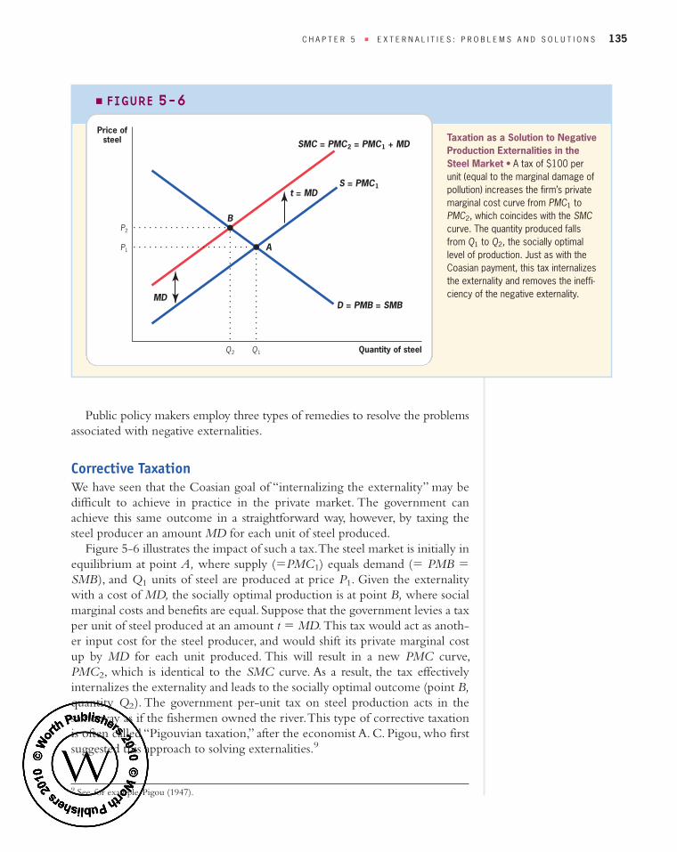
Corrective TaxationWe have seen that the Coasian goal of “internalizing the externality” may bedifficult to achieve in practice in the private market. The government canachieve this same outcome in a straightforward way, however, by taxing thesteel producer an amount MD for each unit of steel produced.

Figure 5-6 illustrates the impact of such a tax. The steel market is initially inequilibrium at point A, where supply (�PMC1) equals demand (� PMB �SMB), and Q1 units of steel are produced at price P1. Given the externalitywith a cost of MD, the socially optimal production is at point B, where socialmarginal costs and benefits are equal. Suppose that the government levies a taxper unit of steel produced at an amount t � MD.This tax would act as anoth-er input cost for the steel producer, and would shift its private marginal costup by MD for each unit produced. This will result in a new PMC curve,PMC2, which is identical to the SMC curve. As a result, the tax effectivelyinternalizes the externality and leads to the socially optimal outcome (point B,quantity Q2). The government per - unit tax on steel production acts in thesame way as if the fishermen owned the river. This type of corrective taxationis often called “Pigouvian taxation,” after the economist A. C. Pigou, who firstsuggested this approach to solving externalities.9


Taxation as a Solution to NegativeProduction Externalities in theSteel Market • A tax of $100 perunit (equal to the marginal damage ofpollution) increases the firm’s privatemarginal cost curve from PMC1 toPMC2, which coincides with the SMCcurve. The quantity produced fallsfrom Q1 to Q2, the socially optimallevel of production. Just as with theCoasian payment, this tax internalizesthe externality and removes the ineffi-ciency of the negative externality.

■ FIGURE 5-6

P1

Quantity of steel

Price ofsteel

Q1Q2

D = PMB = SMBMD

SMC = PMC2 = PMC1 + MD

S = PMC1

A

BP2

t = MD

9 See, for example, Pigou (1947).


SubsidiesAs noted earlier, not all externalities are negative; in cases such as oil explo-ration or nice landscaping by your neighbors, externalities can be positive.

The Coasian solution to cases such as the oil exploration case would be forthe other oil producers to take up a collection to pay the initial driller tosearch for more oil reserves (thus giving them the chance to make moremoney from any oil that is found). But, as we discussed, this may not be feasi-ble. The government can achieve the same outcome by making a payment, ora subsidy, to the initial driller to search for more oil. The amount of this sub-sidy would exactly equal the benefit to the other oil companies and wouldcause the initial driller to search for more oil, since his cost per barrel has beenlowered.

The impact of such a subsidy is illustrated in Figure 5-7, which showsonce again the market for oil exploration. The market is initially in equilibri-um at point A where PMC1 equals PMB, and Q1 barrels of oil are producedat price P1. Given the positive externality with a benefit of MB, the sociallyoptimal production is at point B, where social marginal costs and benefits areequal. Suppose that the government pays a subsidy per barrel of oil producedof S � MB. The subsidy would lower the private marginal cost of oil pro-duction, shifting the private marginal cost curve down by MB for each unitproduced. This will result in a new PMC curve, PMC2, which is identical tothe SMC curve. The subsidy has caused the initial driller to internalize thepositive externality, and the market moves from a situation of underproduc-tion to one of optimal production.


subsidy Government paymentto an individual or firm that low-ers the cost of consumption orproduction, respectively.

Subsidies as a Solution toPositive Production External-ities in the Market for OilExploration • A subsidy that isequal to the marginal benefitfrom oil exploration reduces theoil producer’s marginal costcurve from PMC1 to PMC2,which coincides with the SMCcurve. The quantity producedrises from Q1 to Q2, the sociallyoptimal level of production.

■ FIGURE 5-7

P1

Quantity of oilexploration

Price ofoil exploration

Q1 Q2

P2

MB

Subsidy =MB

D = PMB = SMB

A

B

S = PMC1

SMC = PMC2 =PMC1 – MB


RegulationThroughout this discussion, you may have been asking yourself: Why this fas-cination with prices, taxes, and subsidies? If the government knows where thesocially optimal level of production is, why doesn’t it just mandate that pro-duction take place at that level, and forget about trying to give private actorsincentives to produce at the optimal point? Using Figure 5-6 as an example,why not just mandate a level of steel production of Q2 and be done with it?

In an ideal world, Pigouvian taxation and regulation would be identical.Because regulation appears much more straightforward, however, it has beenthe traditional choice for addressing environmental externalities in the UnitedStates and around the world. When the U.S. government wanted to reduceemissions of sulfur dioxide (SO2) in the 1970s, for example, it did so by put-ting a limit or cap on the amount of sulfur dioxide that producers could emit,not by a tax on emissions. In 1987, when the nations of the world wanted tophase out the use of chlorofluorocarbons (CFCs), which were damaging theozone layer, they banned the use of CFCs rather than impose a large tax onproducts that used CFCs.

Given this governmental preference for quantity regulation, why are econo-mists so keen on taxes and subsidies? In practice, there are complications thatmay make taxes a more effective means of addressing externalities. In the nextsection, we discuss two of the most important complications. In doing so, weillustrate the reasons that policy makers might prefer regulation, or the “quantityapproach” in some situations, and taxation, or the “price approach” in others.

5.4Distinctions Between Price and Quantity Approachesto Addressing Externalities

In this section, we compare price (taxation) and quantity (regulation)approaches to addressing externalities, using more complicated models in

which the social efficiency implications of intervention might differ betweenthe two approaches. The goal in comparing these approaches is to find themost efficient path to environmental targets. That is, for any reduction in pol-lution, the goal is to find the lowest - cost means of achieving that reduction.10

Basic ModelTo illustrate the important differences between the price and quantityapproaches, we have to add one additional complication to the basic competi-tive market that we have worked with thus far. In that model, the only way toreduce pollution was to cut back on production. In reality, there are manyother technologies available for reducing pollution besides simply scaling back


10 The discussion of this section focuses entirely on the efficiency consequences of tax versus regulatoryapproaches to addressing externalities. There may be important equity considerations as well, however,which affect the government’s decision about policy instruments. We will discuss the equity properties oftaxation in Chapter 19.



The Market for Pollution Reduction • The marginal cost of pollution reduction (PMC � SMC) is a rising function, while the marginal benefit of pollution reduction (SMB) is (by assumption) a flat marginaldamage curve. Moving from left to right, the amount of pollution reduction increases, while the amountof pollution falls. The optimal level of pollution reduction is R *, the point at which these curves inter-sect. Since pollution is the complement of reduction, the optimal amount of pollution is P*.

Pollutionreduction ($)(firm’s cost,

society’s benefit)

A

B

S = PMC = SMC

MD = SMB

D = PMB

Reduction 00

More reduction

More pollution

R*

P*Pfull

Rfull

Pollution

■ FIGURE 5-8

production. For example, to reduce sulfur dioxide emissions from coal - firedpower plants, utilities can install smokestack scrubbers that remove SO2 fromthe emissions and sequester it, often in the form of liquid or solid sludge thatcan be disposed of safely. Passenger cars can also be made less polluting byinstalling “catalytic converters,” which turn dangerous nitrogen oxide intocompounds that are not harmful to public health.

To understand the differences between price and quantity approaches topollution reduction, it is useful to shift our focus from the market for a good(e.g., steel) to the “market” for pollution reduction, as illustrated in Figure 5-8.In this diagram, the horizontal axis measures the extent of pollution reductionundertaken by a plant; a value of zero indicates that the plant is not engagingin any pollution reduction. Thus, the horizontal axis also measures the amountof pollution: as you move to the right, there is more pollution reduction andless pollution. We show this by denoting more reduction as you move to theright on the horizontal axis; Rfull indicates that pollution has been reduced tozero. More pollution is indicated as you move to the left on the horizontal axis;at Pfull, the maximum amount of pollution is being produced. The vertical axisrepresents the cost of pollution reduction to the plant, or the benefit of pollu-tion reduction to society (that is, the benefit to other producers and consumerswho are not compensated for the negative externality).


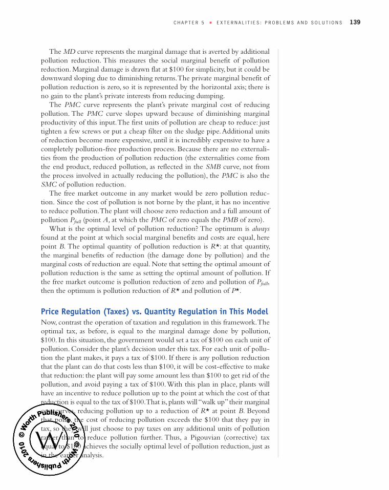
The MD curve represents the marginal damage that is averted by additionalpollution reduction. This measures the social marginal benefit of pollutionreduction. Marginal damage is drawn flat at $100 for simplicity, but it could bedownward sloping due to diminishing returns. The private marginal benefit ofpollution reduction is zero, so it is represented by the horizontal axis; there isno gain to the plant’s private interests from reducing dumping.

The PMC curve represents the plant’s private marginal cost of reducingpollution. The PMC curve slopes upward because of diminishing marginalproductivity of this input. The first units of pollution are cheap to reduce: justtighten a few screws or put a cheap filter on the sludge pipe. Additional unitsof reduction become more expensive, until it is incredibly expensive to have acompletely pollution - free production process. Because there are no externali-ties from the production of pollution reduction (the externalities come fromthe end product, reduced pollution, as reflected in the SMB curve, not fromthe process involved in actually reducing the pollution), the PMC is also theSMC of pollution reduction.

The free market outcome in any market would be zero pollution reduc-tion. Since the cost of pollution is not borne by the plant, it has no incentiveto reduce pollution. The plant will choose zero reduction and a full amount ofpollution P full (point A, at which the PMC of zero equals the PMB of zero).

What is the optimal level of pollution reduction? The optimum is alwaysfound at the point at which social marginal benefits and costs are equal, herepoint B. The optimal quantity of pollution reduction is R*: at that quantity,the marginal benefits of reduction (the damage done by pollution) and themarginal costs of reduction are equal. Note that setting the optimal amount ofpollution reduction is the same as setting the optimal amount of pollution. Ifthe free market outcome is pollution reduction of zero and pollution of Pfull,then the optimum is pollution reduction of R* and pollution of P*.

Price Regulation (Taxes) vs. Quantity Regulation in This ModelNow, contrast the operation of taxation and regulation in this framework. Theoptimal tax, as before, is equal to the marginal damage done by pollution,$100. In this situation, the government would set a tax of $100 on each unit ofpollution. Consider the plant’s decision under this tax. For each unit of pollu-tion the plant makes, it pays a tax of $100. If there is any pollution reductionthat the plant can do that costs less than $100, it will be cost - effective to makethat reduction: the plant will pay some amount less than $100 to get rid of thepollution, and avoid paying a tax of $100. With this plan in place, plants willhave an incentive to reduce pollution up to the point at which the cost of thatreduction is equal to the tax of $100. That is, plants will “walk up” their marginalcost curves, reducing pollution up to a reduction of R* at point B. Beyondthat point, the cost of reducing pollution exceeds the $100 that they pay intax, so they will just choose to pay taxes on any additional units of pollutionrather than to reduce pollution further. Thus, a Pigouvian (corrective) taxequal to $100 achieves the socially optimal level of pollution reduction, just asin the earlier analysis.



Regulation is even more straightforward to analyze in this framework. Thegovernment simply mandates that the plant reduce pollution by an amountR*, to get to the optimal pollution level P*. Regulation seems more difficultthan taxation because, in this case, the government needs to know not onlyMD but also the shape of the MC curve as well. This difficulty is, however, justa feature of our assumption of constant MD; for the more general case of afalling MD, the government needs to know the shapes of both MC and MDcurves in order to set either the optimal tax or the optimal regulation.

Multiple Plants with Different Reduction CostsNow, let’s add two wrinkles to the basic model. First, suppose there are nowtwo steel plants doing the dumping, with each plant dumping 200 units ofsludge into the river each day. The marginal damage done by each unit ofsludge is $100, as before. Second, suppose that technology is now available toreduce sludge associated with production, but this technology has differentcosts at the two different plants. For plant A reducing sludge is cheaper at anylevel of reduction, since it has a newer production process. For the secondplant, B, reducing sludge is much more expensive for any level of reduction.

Figure 5-9 summarizes the market for pollution reduction in this case. Inthis figure, there are separate marginal cost curves for plant A (MCA) and forplant B (MCB ). At every level of reduction, the marginal cost to plant A islower than the marginal cost to plant B, since plant A has a newer and moreefficient production process available. The total marginal cost of reduction inthe market, the horizontal sum of these two curves, is MCT: for any totalreduction in pollution, this curve indicates the cost of that reduction if it isdistributed most efficiently across the two plants. For example, the total mar-ginal cost of a reduction of 50 units is $0, since plant A can reduce 50 units forfree; so the efficient combination is to have plant A do all the reducing. Thesocially efficient level of pollution reduction (and of pollution) is the intersec-tion of this MCT curve with the marginal damage curve, MD, at point Z, indi-cating a reduction of 200 units (and pollution of 200 units).

Policy Option 1: Quantity Regulation Let’s now examine the government’spolicy options within the context of this example. The first option is regula-tion: the government can demand a total reduction of 200 units of sludgefrom the market. The question then becomes: How does the governmentdecide how much reduction to demand from each plant? The typical regula-tory solution to this problem in the past was to ask the plants to split the bur-den: each plant reduces pollution by 100 units to get to the desired totalreduction of 200 units.

This is not an efficient solution, however, because it ignores the fact that theplants have different marginal costs of pollution reduction. At an equal level ofpollution reduction (and pollution), each unit of reduction costs less for plantA (MCA) than for plant B (MCB). If, instead, we got more reduction fromplant A than from plant B, we could lower the total social costs of pollutionreduction by taking advantage of reduction at the low - cost option (plant A).



So society as a whole is worse off if plant A and plant B have to make equalreduction than if they share the reduction burden more efficiently.

This point is illustrated in Figure 5-9. The efficient solution is one where, foreach plant, the marginal cost of reducing pollution is set equal to the social mar-ginal benefit of that reduction; that is, where each plant’s marginal cost curveintersects with the marginal benefit curve. This occurs at a reduction of 50 unitsfor plant B (point X ), and 150 units for plant A (point Y ). Thus, mandating areduction of 100 units from each plant is inefficient; total costs of achieving areduction of 200 units will be lower if plant A reduces by a larger amount.

Policy Option 2: Price Regulation Through a Corrective Tax The secondapproach is to use a Pigouvian corrective tax, set equal to the marginal dam-age, so each plant would face a tax of $100 on each unit of sludge dumped.Faced with this tax, what will each plant do? For plant A, any unit of sludgereduction up to 150 units costs less than $100, so plant A will reduce its pollu-tion by 150 units. For plant B, any unit of sludge reduction up to 50 unitscosts less than $100, so it will reduce pollution by 50 units. Note that these areexactly the efficient levels of reduction! Just as in our earlier analysis, Pigou-vian taxes cause efficient production by raising the cost of the input by the size


Pollution Reduction with Multiple Firms • Plant A has a lower marginal cost of pollution reduction at each level of reduction than does plant B. The optimal level of reduction for the market is the point at which the sum of marginal costs equals marginal damage (at point Z, with a reduction of 200 units). An equal reduction of 100 units for each plant is inefficient since the marginal cost to plant B (MCB) is so much higher than the marginal cost to plant A (MCA). The optimal division of this reduction is where each plant’s marginal cost is equal to the social marginal benefit (which is equal to marginal damage). This occurs when plant A reduces by 150 units and plant B reduces by 50 units, at a marginal cost to each of $100.

Cost ofpollution

reduction ($)

X Y Z

Reduction100

0

500 150 200 400

MD = SMB

MCTMCA

MCB

MCB,100

MCA,100

Pollution300

350400 250 200 0

$100

■ FIGURE 5-9


of its external damage, thereby raising private marginal costs to social marginalcosts. Taxes are preferred to quantity regulation, with an equal distribution ofreductions across the plants, because taxes give plants more flexibility inchoosing their optimal amount of reduction, allowing them to choose theefficient level.

Policy Option 3: Quantity Regulation with Tradable Permits Does thismean that taxes always dominate quantity regulation with multiple plants? Notnecessarily. If the government had mandated the appropriate reduction fromeach plant (150 units from A and 50 units from B), then quantity regulationwould have achieved the same outcome as the tax. Such a solution would,however, require much more information. Instead of just knowing the mar-ginal damage and the total marginal cost, the government would also have toknow the marginal cost curves of each individual plant. Such detailed infor-mation would be hard to obtain.

Quantity regulation can be rescued, however, by adding a key flexibility:issue permits that allow a certain amount of pollution and let the plants trade.Suppose the government announces the following system: it will issue 200permits that entitle the bearer to produce one unit of pollution. It will initiallyprovide 100 permits to each plant. Thus, in the absence of trading, each plantwould be allowed to produce only 100 units of sludge, which would in turnrequire each plant to reduce its pollution by half (the inefficient solution pre-viously described).

If the government allows the plants to trade these permits to each other,however, plant B would have an interest in buying permits from plant A. Forplant B, reducing sludge by 100 units costs MCB,100, a marginal cost muchgreater than plant A’s marginal cost of reducing pollution by 100 units, which isMCA,100. Thus, plants A and B can be made better off if plant B buys a permitfrom plant A for some amount between MCA,100 and MCB,100, so that plant Bwould pollute 101 units (reducing only 99 units) and plant A would pollute99 units (reducing 101 units). This transaction is beneficial for plant B because aslong as the cost of a permit is below MCB,100, plant B pays less than the amountit would cost plant B to reduce the pollution on its own. The trade is beneficialfor plant A as long as it receives for a permit at least MCA,100, since it can reducethe sludge for a cost of only MCA,100, and make money on the difference.

By the same logic, a trade would be beneficial for a second permit, so thatplant B could reduce sludge by only 98, and plant A would reduce by 102. Infact, any trade will be beneficial until plant B is reducing by 50 units and plantA is reducing by 150 units. At that point, the marginal costs of reduction acrossthe two producers are equal (to $100), so that there are no more gains fromtrading permits.

What is going on here? We have simply returned to the intuition of theCoasian solution: we have internalized the externality by providing property rightsto pollution. So, like Pigouvian taxes, trading allows the market to incorporatedifferences in the cost of pollution reduction across firms. In Chapter 6, wediscuss a successful application of trading to the problem of environmentalexternalities.



Uncertainty About Costs of ReductionDifferences in reduction costs across firms are not the only reason that taxes orregulation might be preferred. Another reason is that the costs or benefits ofregulation could be uncertain. Consider two extreme examples of externali-ties: global warming and nuclear leakage. Figure 5-10 extends the pollutionreduction framework from Figure 5-8 to the situation in which the marginal


Market for PollutionReduction with UncertainCosts • In the case of global warming (panel (a)),the marginal damage is fairly constant over largeranges of emissions (andthus emission reductions). If costs are uncertain, thentaxation at level t � C2

leads to a much lowerdeadweight loss (DBE) thandoes regulation of R1 (ABC).In the case of nuclear leak-age (panel (b)), the marginaldamage is very steep. Ifcosts are uncertain, thentaxation leads to a muchlarger deadweight loss(DBE) than does regulation(ABC).

Cost ofpollution

reduction ($)

Cost ofpollution

reduction ($)

MC2

MC1

DWL1

DWL2

D B

A

CE MD = SMB

C1

A

MD = SMB

MC2

MC1

C

E

B

D

C1DWL1

DWL2

(a) Global warming

(b) Nuclear leakage

Reduction 00Pfull

R fullR2 R1R3

P2 P1P3Pollution

Taxation = C2

Reduction 00Pfull

R fullR2 R1R3

P2 P1P3Pollution

t = C2

Mandated

■ FIGURE 5-10


damage (which is equal to the marginal social benefit of pollution reduction)is now no longer constant, but falling. That is, the benefit of the first unit ofpollution reduction is quite high, but once the production process is relativelypollution - free, additional reductions are less important (that is, there arediminishing marginal returns to reduction).

Panel (a) of Figure 5-10 considers the case of global warming. In this case,the exact amount of pollution reduction is not so critical for the environment.Since what determines the extent of global warming is the total accumulatedstock of carbon dioxide in the air, which accumulates over many years fromsources all over the world, even fairly large shifts in carbon dioxide pollution inone country today will have little impact on global warming. In that case, wesay that the social marginal benefit curve (which is equal to the marginal dam-age from global warming) is very flat: that is, there is little benefit to societyfrom modest additional reductions in carbon dioxide emissions.

Panel (b) of Figure 5-10 considers the case of radiation leakage from anuclear power plant. In this case, a very small difference in the amount ofnuclear leakage can make a huge difference in terms of lives saved. Indeed, it ispossible that the marginal damage curve (which is once again equal to themarginal social benefits of pollution reduction) for nuclear leakage is almostvertical, with each reduction in leakage being very important in terms of sav-ing lives. Thus, the social marginal benefit curve in this case is very steep.

Now, in both cases, imagine that we don’t know the true costs of pollutionreduction on the part of firms or individuals. The government’s best guess isthat the true marginal cost of pollution reduction is represented by curveMC1 in both panels. There is a chance, however, that the marginal cost of pol-lution reduction could be much higher, as represented by the curve MC2. Thisuncertainty could arise because the government has an imperfect understand-ing of the costs of pollution reduction to the firm, or it could arise becauseboth the government and the firms are uncertain about the ultimate costs ofpollution reduction.

Implications for Effect of Price and Quantity Interventions This uncer-tainty over costs has important implications for the type of intervention thatreduces pollution most efficiently in each of these cases. Consider regulationfirst. Suppose that the government mandates a reduction, R1, which is theoptimum if costs turn out to be given by MC1: this is where social marginalbenefits equal social marginal costs of reduction if marginal cost equals MC1.Suppose now that the marginal costs actually turn out to be MC2, so that theoptimal reduction should instead be R2, where SMB � MC2. That is, regula-tion is mandating a reduction in pollution that is too large, with the marginalbenefits of the reduction being below the marginal costs. What are the efficiencyimplications of this mistake?

In the case of global warming (panel (a)), these efficiency costs are quitehigh. With a mandated reduction of R1, firms will face a cost of reduction ofC1, the cost of reducing by amount R1 if marginal costs are described byMC2. The social marginal benefit of reduction of R1 is equal to C2, the pointwhere R1 intersects the SMB curve. Since the cost to firms (C1) is so much



higher than the benefit of reduction (C2), there is a large deadweight loss(DWL1) of area ABC (the triangle that incorporates all units where cost ofreduction exceeds benefits of reduction).

In the case of nuclear leakage (panel (b)), the costs of regulation are very low.Once again, with a mandated reduction of R1, firms will face a cost of reduc-tion of C1, the cost of reducing by amount R1 if marginal costs are describedby MC2. The social marginal benefit of reduction at R1 is once again equal toC2. In this case, however, the associated deadweight loss triangle ABC (DWL1)is much smaller than in panel (a), so the inefficiency from regulation is muchlower.

Now, contrast the use of corrective taxation in these two markets. Supposethat the government levies a tax designed to achieve the optimal level ofreduction if marginal costs are described in both cases by MC1, which is R1.As discussed earlier, the way to do this is to choose a tax level, t, such that thefirm chooses a reduction of R1. In both panels, the tax level that will causefirms to choose reduction R1 is a tax equal to C2, where MC1 intersects MD.A tax of this amount would cause firms to do exactly R1 worth of reduction,if marginal costs are truly determined by MC1.

If the true marginal cost ends up being MC2, however, the tax causes firmsto choose a reduction of R3, where their true marginal cost is equal to the tax(where t � MC2 at point E), so that there is too little reduction. In the case ofglobal warming in panel (a), the deadweight loss (DWL2) from reducing by R3

instead of R2 is only the small area DBE, representing the units where socialmarginal benefits exceed social marginal costs. In the case of nuclear leakage inpanel (b), however, the deadweight loss (DWL2) from reducing by R3 instead ofR2 is a much larger area, DBE, once again representing the units where socialmarginal benefits exceed social marginal costs.

Implications for Instrument Choice The central intuition here is that theinstrument choice depends on whether the government wants to get the amount of pollu-tion reduction right or whether it wants to minimize costs. Quantity regulationassures there is as much reduction as desired, regardless of the cost. So, if it iscritical to get the amount exactly right, quantity regulation is the best way togo. This is why the efficiency cost of quantity regulation under uncertainty is somuch lower with the nuclear leakage case in panel (b). In this case, it is criticalto get the reduction close to optimal; if we end up costing firms extra money inthe process, so be it. For global warming, getting the reduction exactly rightisn’t very important; so it is inefficient in this case to mandate a very costlyoption for firms.

Price regulation through taxes, on the other hand, assures that the cost ofreductions never exceeds the level of the tax, but leaves the amount of reduc-tion uncertain. That is, firms will never reduce pollution beyond the point atwhich reductions cost more than the tax they must pay (the point at whichthe tax intersects their true marginal cost curve, MC2). If marginal costs turnout to be higher than anticipated, then firms will just do less pollution reduc-tion. This is why the deadweight loss of price regulation in the case of globalwarming is so small in panel (a): the more efficient outcome is to get the exact



reduction wrong but protect firms against very high costs of reduction. This isclearly not true in panel (b): for nuclear leakage, it is most important to get thequantity close to right (almost) regardless of the cost to firms.

In summary, quantity regulations ensure environmental protection, but at avariable cost to firms, while price regulations ensure the cost to the firms, butat a variable level of environmental protection. So, if the value of getting theenvironmental protection close to right is high, then quantity regulations willbe preferred; but if getting the protection close to right is not so important,then price regulations are a preferred option.

5.5Conclusion

Externalities are the classic answer to the “when” question of public finance:when one party’s actions affect another party, and the first party doesn’t

fully compensate (or get compensated by) the other for this effect, then themarket has failed and government intervention is potentially justified. Insome cases, the market is likely to find a Coasian solution whereby negotia-tions between the affected parties lead to the “internalization” of the exter-nality. For many cases, however, only government intervention can solve themarket failure.

This point naturally leads to the “how” question of public finance. Thereare two classes of tools in the government’s arsenal for dealing with externali-ties: price - based measures (taxes and subsidies) and quantity - based measures(regulation). Which of these methods will lead to the most efficient regulatoryoutcome depends on factors such as the heterogeneity of the firms being reg-ulated, the flexibility embedded in quantity regulation, and the uncertaintyover the costs of externality reduction. In the next chapter, we take thesesomewhat abstract principles and apply them to some of the most importantexternalities facing the United States (and the world) today.


an unlikely solution to global externalities, such asmost environmental externalities.

■ The government can use either price (tax or sub-sidy) or quantity (regulation) approaches to address-ing externalities.

■ When firms have different marginal costs of pollu-tion reduction, price mechanisms are a more effi-cient means of accomplishing environmental goalsunless quantity regulation is accompanied by theability to meet regulatory targets by trading pollu-tion permits across polluters.

■ Externalities arise whenever the actions of oneparty make another party worse or better off, yetthe first party neither bears the costs nor receivesthe benefits of doing so.

■ Negative externalities cause overproduction of thegood in a competitive market, while positive external-ities cause underproduction of the good in a competi-tive market, in both cases leading to a deadweight loss.

■ Private markets may be able to “internalize” theproblems of externalities through negotiation, butthis Coasian process faces many barriers that make it

� H I G H L I G H T S



town where it operates: the marginal external costassociated with the Qth unit of production isgiven by 6Q. What is the marginal private costassociated with the 10th unit produced? What isthe total marginal cost to society associated withproducing the 10th unit (the marginal social costof the 10th unit)?

8. In two - car automobile accidents, passengers in thelarger vehicle are significantly more likely to sur-vive than are passengers in the smaller vehicle. Infact, death probabilities are decreasing in the sizeof the vehicle you are driving, and death probabil-ities are increasing in the size of the vehicle youcollide with. Some politicians and lobbyists haveargued that this provides a rationale for encourag-ing the sale of larger vehicles and discouraginglegislation that would induce automobile manu-facturers to make smaller cars. Critically examinethis argument using the concept of externalities.

9. Why do governments sometimes impose quantityregulations that limit the level of negative - externality - inducing consumption? Why do gov-ernments sometimes impose price regulations bytaxing this consumption?

10. Answer the following two questions for each ofthe following examples: (i) smoking by individu-als; (ii) toxic waste production by firms; (iii)research and development by a high - tech firm;and (iv) individual vaccination against communi-cable illness.a. Is there an externality? If so, describe it, includ-

ing references to whether it is positive or nega-tive, and whether it is a consumption orproduction externality.

b. If there is an externality, does it seem likely thatprivate markets will arise that allow this exter-nality to be internalized? Why or why not?

1. Peterson, Hoffer, and Millner (1995) showed thatair bag use has led to increases in car crashes.Despite this finding, the government mandatesthat new cars have air bags, rather than taxingtheir use. Is this policy a contradiction?

2. When the state of Virginia imposed stricter regu-lations on air pollution in 2003, it also authorizedan auction of pollution permits, allowing someplants to emit larger amounts of ozone - depletingchemicals than would otherwise be allowed, andsome to emit less. Theory predicts that this auc-tion led to a socially efficient allocation of pollu-tion. Describe how this outcome would occur.

3. Can an activity generate both positive and nega-tive externalities at the same time? Explain youranswer.

4. In the midwestern United States, where windstend to blow from west to east, states tend to moreeasily approve new polluting industries near theireastern borders than in other parts of the state.Why do you think this is true?

5. Can government assignment and enforcement ofproperty rights internalize an externality? Willthis approach work as well as, better than, orworse than direct government intervention?Explain your answers and describe one of the dif-ficulties associated with this solution.

6. In close congressional votes, many members ofCongress choose to remain “undecided” until thelast moment. Why might they do this? What les-son does this example teach about a potentialshortcoming of the Coasian solution to the exter-nality problem?

7. Suppose that a firm’s marginal production costsare given by MC � 10 � 3Q. The firm’s produc-tion process generates a toxic waste, which imposesan increasingly large cost on the residents of the

� Q U E S T I O N S A N D P R O B L E M S

■ If there is uncertainty about the marginal costs ofpollution reduction, then the relative merits of priceand quantity regulations will depend on the steep-ness of the marginal benefit curve. Quantity regula-tion gets the amount of pollution reduction right,

regardless of cost, and so is more appropriate whenmarginal benefits are steep; price regulation throughtaxation gets the costs of pollution reduction right,regardless of quantity, so it is more appropriatewhen marginal benefits are flat.



common tax per unit of pollution; or (3) requireall firms to reduce pollution by the sameamount, but allow pollution permits to bebought and sold.

16. One hundred commuters need to use a strip ofhighway to get to work. They all drive alone andprefer to drive in big cars—it gives them moreprestige and makes them feel safer. Bigger carscost more per mile to operate, however, sincetheir gas mileage is lower. Worse yet, bigger carscause greater permanent damage to roads.

The weight of the car is w. Suppose that thebenefits from driving are 4w, while the costs are3/2 � w2. The damage to roads is 1/3 � w3.Assume that individuals have utility functions ofthe form U � x, where x are the net benefitsfrom driving a car of a given size.

a. What car weight will be chosen by drivers?b. What is the optimal car weight? If this differs

from (a), why does it?c. Can you design a toll system that causes drivers

to choose the optimal car weight? If so, thenhow would such a system work?

17. Firms A and B each produce 80 units of pollution.The federal government wants to reduce pollu-tion levels. The marginal costs associated with pol-lution reduction are MCA � 50 � 3QA for firmA and MCB � 20 � 6QB for firm B, where QA

and QB are the quantities of pollution reduced byeach firm. Society’s marginal benefit from pollu-tion reduction is given by MB � 590 � 3QT,where QT is the total reduction in pollution.

a. What is the socially optimal level of each firm’spollution reduction?

b. How much total pollution is there in the socialoptimum?

c. Explain why it is inefficient to give each firman equal number of pollution permits (if theyare not allowed to trade them).

d. Explain how the social optimum can beachieved if firms are given equal numbers ofpollution permits but are allowed to trade them.

e. Can the social optimum be achieved using atax on pollution?

11. Warrenia has two regions. In Oliviland, the mar-ginal benefit associated with pollution cleanup isMB � 300 � 10Q, while in Linneland, the mar-ginal benefit associated with pollution cleanup isMB � 200 � 4Q. Suppose that the marginal costof cleanup is constant at $12 per unit. What is theoptimal level of pollution cleanup in each of thetwo regions?

12. The private marginal benefit associated with aproduct’s consumption is PMB � 360 � 4Q andthe private marginal cost associated with its pro-duction is PMC � 6P. Furthermore, the marginalexternal damage associated with this good’s pro-duction is MD � 2P. To correct the externality,the government decides to impose a tax of T perunit sold. What tax T should it set to achieve thesocial optimum?

13. Suppose that demand for a product is Q � 1200 �4P and supply is Q � �200 � 2P. Furthermore,suppose that the marginal external damage of thisproduct is $8 per unit. How many more units ofthis product will the free market produce than issocially optimal? Calculate the deadweight lossassociated with the externality.

14. The marginal damage averted from pollutioncleanup is MD � 200 � 5Q. The marginal costassociated with pollution cleanup is MC � 10 � Q.

a. What is the optimal level of pollution reduction?b. Show that this level of pollution reduction

could be accomplished through taxation. Whattax per unit would generate the optimal amountof pollution reduction?

15. Two firms are ordered by the federal governmentto reduce their pollution levels. Firm A’s marginalcosts associated with pollution reduction is MC �20 � 4Q. Firm B’s marginal costs associated withpollution reduction is MC � 10 � 8Q. The mar-ginal benefit of pollution reduction is MB � 400 �4Q.

a. What is the socially optimal level of each firm’spollution reduction?

b. Compare the social efficiency of three possi-ble outcomes: (1) require all firms to reducepollution by the same amount; (2) charge a

� A DVA N C E D Q U E S T I O N S


5.1 Externality Theory to Negative Externalities ... · PDF fileExternalities: Problems and...

Documents

Transcript of 5.1 Externality Theory to Negative Externalities ... · PDF fileExternalities: Problems and...