
5. Sample Size, Power & Thresholdspages.stat.wisc.edu/~yandell/statgen/course/notes/course5.pdf ·...
22
ch. 5 © 2003 Broman, Churchill, Yandell, Zeng 1 5. Sample Size, Power & Thresholds • review of sample size for t-test (known QTL) • sample size, marker spacing & power – Zeng talk at Plant & Animal Genome XI, 2003 (statgen.ncsu.edu/zeng/QTLPower-Presentation.pdf) • QTL thresholds & genome-wide error rates • positive false detection rates • selection bias ch. 5 © 2003 Broman, Churchill, Yandell, Zeng 2 5.1 review sample size for t-test • set up test under "null hypothesis" of no QTL – two-sided test for difference – size arbitrary--usually α = .05 • determine power or sample size under alternative – power = chance to reject null if alternative true – sample size (n/4 per MM,mm) follows square root idea 2 2 / ] / ) [( 2 1 ) QTL | ( pr : power 2 / ) QTL no | ( pr : size/2 / 8 d z z n c c SE d n t mm MM mm MM mm MM σ β µ µ α µ µ σ µ µ β α + = − = > − = > − = − =
Transcript of 5. Sample Size, Power & Thresholdspages.stat.wisc.edu/~yandell/statgen/course/notes/course5.pdf ·...
ch. 5 © 2003 Broman, Churchill, Yandell, Zeng 1
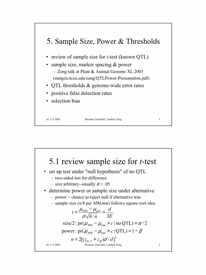
5. Sample Size, Power & Thresholds
• review of sample size for t-test (known QTL)• sample size, marker spacing & power
– Zeng talk at Plant & Animal Genome XI, 2003(statgen.ncsu.edu/zeng/QTLPower-Presentation.pdf)
• QTL thresholds & genome-wide error rates• positive false detection rates• selection bias
ch. 5 © 2003 Broman, Churchill, Yandell, Zeng 2
5.1 review sample size for t-test• set up test under "null hypothesis" of no QTL
– two-sided test for difference– size arbitrary--usually α = .05
• determine power or sample size under alternative– power = chance to reject null if alternative true– sample size (n/4 per MM,mm) follows square root idea
22/ ]/)[(2
1)QTL |(pr:power2/)QTL no |(pr:size/2
/8
dzzncc
SEd
nt
mmMM
mmMM
mmMM
σβµµαµµ
σµµ
βα +=
−=>−=>−
=−=
ch. 5 © 2003 Broman, Churchill, Yandell, Zeng 3
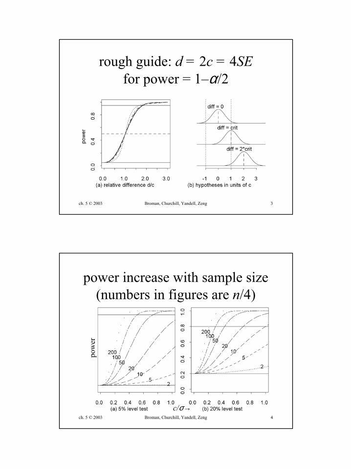
rough guide: d = 2c = 4SEfor power = 1–α/2
ch. 5 © 2003 Broman, Churchill, Yandell, Zeng 4
power increase with sample size(numbers in figures are n/4)
pow
er
c/σ→
ch. 5 © 2003 Broman, Churchill, Yandell, Zeng 5
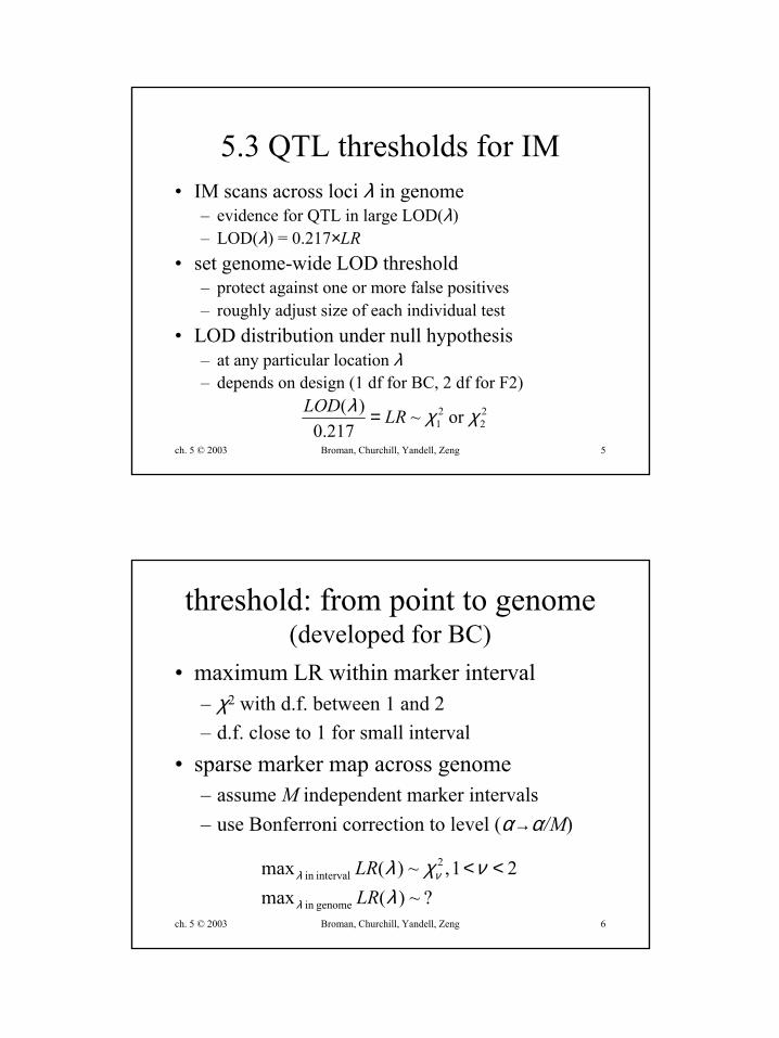
5.3 QTL thresholds for IM• IM scans across loci λ in genome
– evidence for QTL in large LOD(λ)– LOD(λ) = 0.217×LR
• set genome-wide LOD threshold– protect against one or more false positives– roughly adjust size of each individual test
• LOD distribution under null hypothesis– at any particular location λ– depends on design (1 df for BC, 2 df for F2)
22
21 or ~
217.0)( χχλ LRLOD =
ch. 5 © 2003 Broman, Churchill, Yandell, Zeng 6
threshold: from point to genome(developed for BC)
• maximum LR within marker interval– χ2 with d.f. between 1 and 2– d.f. close to 1 for small interval
• sparse marker map across genome– assume M independent marker intervals– use Bonferroni correction to level (α→α/M)
?~)(max21 ,~)(max
genome in
2interval in
λνχλ
λ
νλ
LRLR <<
ch. 5 © 2003 Broman, Churchill, Yandell, Zeng 7
LR, LOD and point-wise p-values
p-value p-valueLR LOD 1 d.f. 2 d.f.10 1 0.0319 0.131.6 1.5 0.0086 0.0316100 2 0.0024 0.011000 3 0.0002 0.00110000 4 <0.0001 0.0001
ch. 5 © 2003 Broman, Churchill, Yandell, Zeng 8
genome-wide threshold: theory• dense marker map: markers everywhere• LR test statistics are correlated
– correlation drops off quickly with distance– no correlation for unlinked markers
• theory: Ohrnstein-Uhlenbeck process– C = number of chromosomes,– G = length of genome in cM– t = genome-wide threshold value– αt= corresponding point-wise significance level
t
t
t
GtCtLR
αχ
ααλλ
=>
+≈=>
)(pr with
)2())((maxpr21
genome in
ch. 5 © 2003 Broman, Churchill, Yandell, Zeng 9
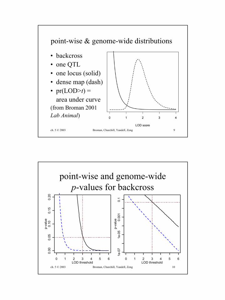
point-wise & genome-wide distributions
• backcross• one QTL• one locus (solid)• dense map (dash)• pr(LOD>t) =
area under curve(from Broman 2001Lab Animal)
ch. 5 © 2003 Broman, Churchill, Yandell, Zeng 10
point-wise and genome-widep-values for backcross
0 1 2 3 4 5 6
0.00
0.05
0.10
0.15
0.20
LOD threshold
p-va
lue
0 1 2 3 4 5 6
1e-0
71e
-05
0.00
10.
1
LOD threshold
p-va
lue
ch. 5 © 2003 Broman, Churchill, Yandell, Zeng 11
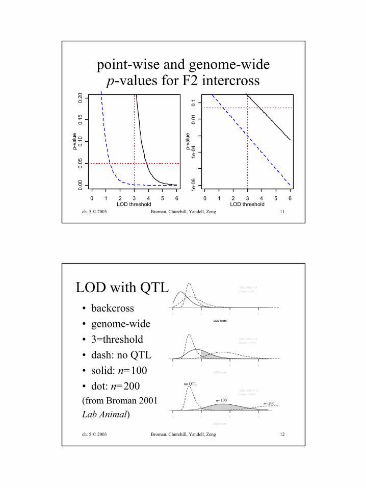
point-wise and genome-widep-values for F2 intercross
0 1 2 3 4 5 6
0.00
0.05
0.10
0.15
0.20
LOD threshold
p-va
lue
0 1 2 3 4 5 61e
-06
1e-0
40.
010.
1
LOD threshold
p-va
lue
ch. 5 © 2003 Broman, Churchill, Yandell, Zeng 12
LOD with QTL• backcross• genome-wide• 3=threshold• dash: no QTL• solid: n=100• dot: n=200(from Broman 2001Lab Animal)
n=100n=200
no QTL
ch. 5 © 2003 Broman, Churchill, Yandell, Zeng 13
5.4 false detection rates and thresholds
• threshold: test QTL across genome– size = pr( LOD(λ) > threshold | no QTL at λ )– guards against a single false detection
• very conservative on genome-wide basis
– difficult to extend to multiple QTL
• positive false discovery rate (Storey 2001)– pFDR = pr( no QTL at λ | LOD(λ) > threshold )– post-hoc estimate of proportion of false positives– easily extended to multiple QTL in Bayesian context
ch. 5 © 2003 Broman, Churchill, Yandell, Zeng 14
pFDR for interval mapping• pFDR = pr(no QTL)*size
pr(no QTL)*size+pr(QTL)*power
• decide on threshold (e.g. genome-wide)• power = pr( LOD(λ) > threshold | QTL at λ )
– proportion of genome with LOD > threshold• size = pr( LOD(λ) > threshold | no QTL at λ )
– point-wise p-value of threshold• prior = pr( no QTL at λ )
– proportion of genome with LOD < "small value"– divided by point-wise p-value for "small value"
ch. 5 © 2003 Broman, Churchill, Yandell, Zeng 15
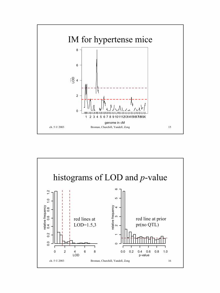
IM for hypertense mice
0
2
4
6
8
lod
1 2 3 4 5 6 7 8 9 10111213141516171819X
genome in cM
LOD
ch. 5 © 2003 Broman, Churchill, Yandell, Zeng 16
0 2 4 6 8
0.0
0.2
0.4
0.6
0.8
1.0
1.2
LOD
rela
tive
frequ
ency
0.0 0.2 0.4 0.6 0.8 1.0
01
23
45
6
p-value
rela
tive
frequ
ency
histograms of LOD and p-value
red line at priorpr(no QTL)
red lines atLOD=1.5,3
ch. 5 © 2003 Broman, Churchill, Yandell, Zeng 17
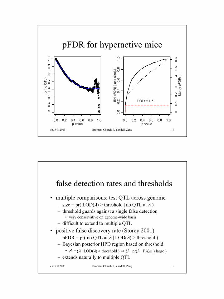
pFDR for hyperactive mice
0.0 0.2 0.4 0.6 0.8 1.0
0.3
0.4
0.5
0.6
0.7
0.8
0.9
1.0
p-value
pr(n
o Q
TL)
0.0 0.2 0.4 0.6 0.8 1.00.
00.
20.
40.
60.
81.
0
p-value
BH p
FDR
(-) a
nd s
ize(
.)
00.
10.
20.
30.
40.
50.
6St
orey
pFD
R(-)
LOD = 1.5
ch. 5 © 2003 Broman, Churchill, Yandell, Zeng 18
false detection rates and thresholds• multiple comparisons: test QTL across genome
– size = pr( LOD(λ) > threshold | no QTL at λ )– threshold guards against a single false detection
• very conservative on genome-wide basis– difficult to extend to multiple QTL
• positive false discovery rate (Storey 2001)– pFDR = pr( no QTL at λ | LOD(λ) > threshold )– Bayesian posterior HPD region based on threshold
• Λ ={λ | LOD(λ) > threshold } ≈ {λ | pr(λ | Y,X,m ) large }– extends naturally to multiple QTL
ch. 5 © 2003 Broman, Churchill, Yandell, Zeng 19
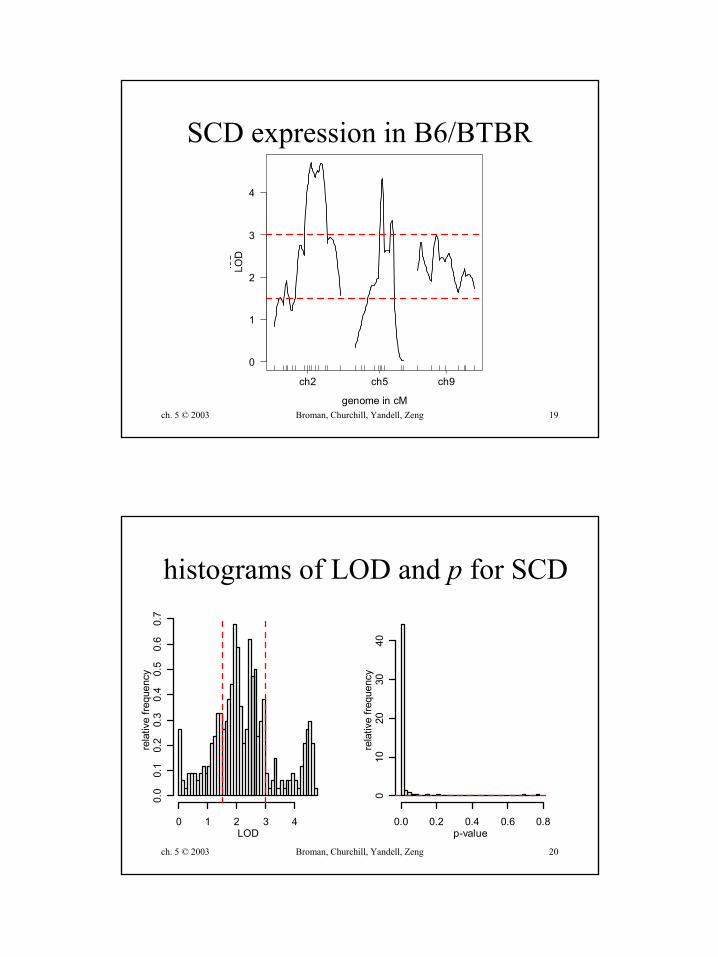
SCD expression in B6/BTBR
0
1
2
3
4
lod
ch2 ch5 ch9
genome in cM
LOD
ch. 5 © 2003 Broman, Churchill, Yandell, Zeng 20
histograms of LOD and p for SCD
0 1 2 3 4
0.0
0.1
0.2
0.3
0.4
0.5
0.6
0.7
LOD
rela
tive
frequ
ency
0.0 0.2 0.4 0.6 0.8
010
2030
40
p-value
rela
tive
frequ
ency
ch. 5 © 2003 Broman, Churchill, Yandell, Zeng 21
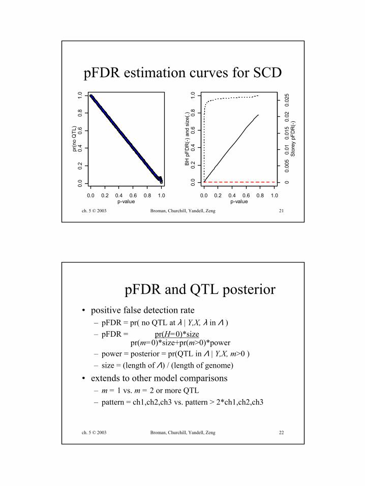
pFDR estimation curves for SCD
0.0 0.2 0.4 0.6 0.8 1.0
0.0
0.2
0.4
0.6
0.8
1.0
p-value
pr(n
o Q
TL)
0.0 0.2 0.4 0.6 0.8 1.00.
00.
20.
40.
60.
81.
0
p-value
BH p
FDR
(-) a
nd s
ize(
.)
00.
005
0.01
0.01
50.
020.
025
Stor
ey p
FDR
(-)
ch. 5 © 2003 Broman, Churchill, Yandell, Zeng 22
pFDR and QTL posterior• positive false detection rate
– pFDR = pr( no QTL at λ | Y,X, λ in Λ )– pFDR = pr(H=0)*size
pr(m=0)*size+pr(m>0)*power– power = posterior = pr(QTL in Λ | Y,X, m>0 )– size = (length of Λ) / (length of genome)
• extends to other model comparisons– m = 1 vs. m = 2 or more QTL– pattern = ch1,ch2,ch3 vs. pattern > 2*ch1,ch2,ch3
ch. 5 © 2003 Broman, Churchill, Yandell, Zeng 23
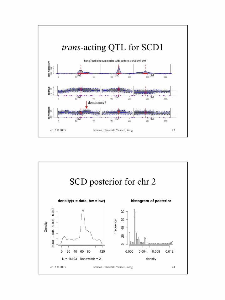
trans-acting QTL for SCD1
dominance?
ch. 5 © 2003 Broman, Churchill, Yandell, Zeng 24
SCD posterior for chr 2
0 20 40 60 80 120
0.00
00.
004
0.00
80.
012
density(x = data, bw = bw)
N = 16103 Bandwidth = 2
Den
sity
histogram of posterior
density
Freq
uenc
y
0.000 0.004 0.008 0.012
020
4060
80
ch. 5 © 2003 Broman, Churchill, Yandell, Zeng 25
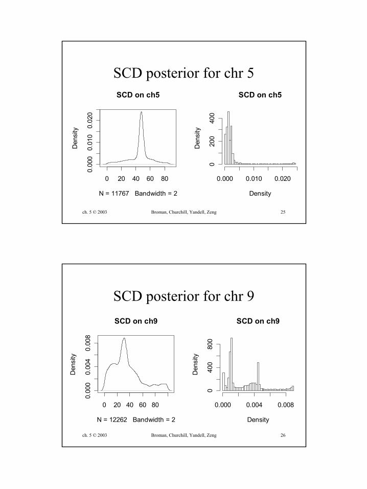
SCD posterior for chr 5
0 20 40 60 80
0.00
00.
010
0.02
0SCD on ch5
N = 11767 Bandwidth = 2
Den
sity
SCD on ch5
DensityD
ensi
ty
0.000 0.010 0.020
020
040
0
ch. 5 © 2003 Broman, Churchill, Yandell, Zeng 26
SCD posterior for chr 9
0 20 40 60 80
0.00
00.
004
0.00
8
SCD on ch9
N = 12262 Bandwidth = 2
Den
sity
SCD on ch9
Density
Den
sity
0.000 0.004 0.008
040
080
0
ch. 5 © 2003 Broman, Churchill, Yandell, Zeng 27
0.0 0.2 0.4 0.6 0.8 1.0
0.0
0.2
0.4
0.6
0.8
1.0
relative size of HPD region
pr( H
=0 |
p>si
ze )
0.0 0.2 0.4 0.6 0.8 1.00.
00.
20.
40.
60.
81.
0
pr( locus in HPD | m>0 )
BH p
FDR
(-) a
nd s
ize(
.)
00.
10.
20.
3St
orey
pFD
R(-)
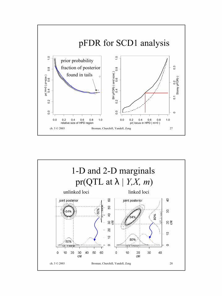
prior probabilityfraction of posterior
found in tails
pFDR for SCD1 analysis
ch. 5 © 2003 Broman, Churchill, Yandell, Zeng 28
1-D and 2-D marginalspr(QTL at λ | Y,X, m)
unlinked loci linked loci
ch. 5 © 2003 Broman, Churchill, Yandell, Zeng 29
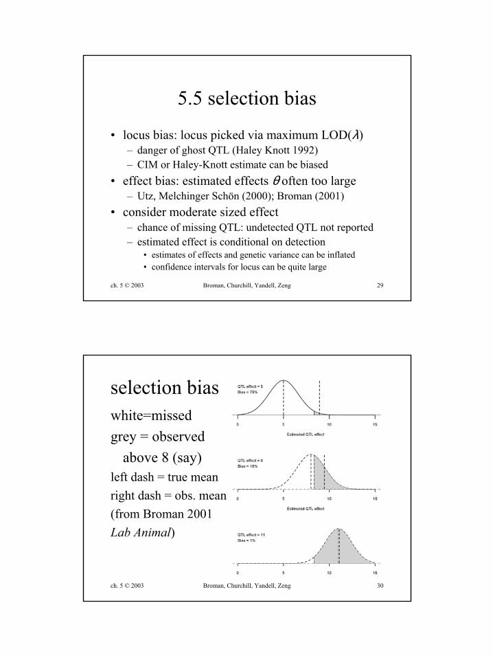
5.5 selection bias
• locus bias: locus picked via maximum LOD(λ)– danger of ghost QTL (Haley Knott 1992)– CIM or Haley-Knott estimate can be biased
• effect bias: estimated effects θ often too large– Utz, Melchinger Schön (2000); Broman (2001)
• consider moderate sized effect– chance of missing QTL: undetected QTL not reported– estimated effect is conditional on detection
• estimates of effects and genetic variance can be inflated• confidence intervals for locus can be quite large
ch. 5 © 2003 Broman, Churchill, Yandell, Zeng 30
selection biaswhite=missedgrey = observed
above 8 (say)left dash = true meanright dash = obs. mean(from Broman 2001Lab Animal)
ch. 5 © 2003 Broman, Churchill, Yandell, Zeng 31
independent validation
• separate study on same parent lines– Beavis (1994) simulation study– Beavis et al. (1994 Crop Sci) field study– Melchinger et al. (1998 Genetics) field study
• resampling evaluation– Beavis (1994) simulation study– Visscher et al. (1996) bootstrap– Utz et al. (2000 Genetics) cross validation`
ch. 5 © 2003 Broman, Churchill, Yandell, Zeng 32
many QTL of small effect?• repeated field studies yield different QTL
– environment effect?– genetic differences: parents, independent cross?– chance variation?
• simulation studies (Beavis 1994, 1998)– 10 QTL of same size– only chance variation– repeated trials yield different QTL again
ch. 5 © 2003 Broman, Churchill, Yandell, Zeng 33
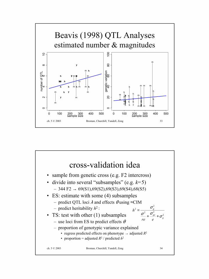
Beavis (1998) QTL Analysesestimated number & magnitudes
0 100 200 300 400 500
02
46
810
sample size
num
ber o
f QTL
m
m
m
m
m
m
m
m
m
m m
mhh
hh
hh
hh
hh
hh
hh
hhhh
hh
hh
yyyy
yy
yy
yy
yy
yyyy
0 100 200 300 400 500
020
4060
8010
0
sample size
gene
tic v
aria
tion
m
m
m
m
m
m
m
m
m
m
m
m
h
h
h
h
h
h
h
h
h
h
h
h
hh
h
h
h
h
h
h
h
h
y
y
y
y
y
yyyy
y
y
y
ch. 5 © 2003 Broman, Churchill, Yandell, Zeng 34
cross-validation idea• sample from genetic cross (e.g. F2 intercross)• divide into several “subsamples” (e.g. k=5)
– 344 F2 → 69(S1),69(S2),69(S3),69(S4),68(S5)• ES: estimate with some (4) subsamples
– predict QTL loci λ and effects θ using ≈CIM– predict heritability h2 :
• TS: test with other (1) subsamples– use loci from ES to predict effects θ– proportion of genotypic variance explained
• regress predicted effects on phenotype → adjusted R2
• proportion = adjusted R2 / predicted h2
222
22
gge
g
ere
hσ
σσσ
++=
ch. 5 © 2003 Broman, Churchill, Yandell, Zeng 35
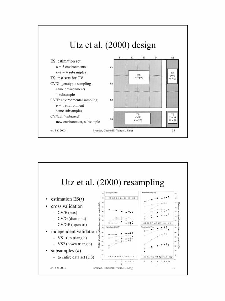
Utz et al. (2000) designES: estimation set
u = 3 environmentsk–1 = 4 subsamples
TS: test sets for CVCV/G: genotypic sampling
same environments1 subsample
CV/E: environmental samplinge = 1 environmentsame subsamples
CV/GE: “unbiased”new environment, subsample
ch. 5 © 2003 Broman, Churchill, Yandell, Zeng 36
Utz et al. (2000) resampling
• estimation ES(•)• cross validation
– CV/E (box)– CV/G (diamond)– CV/GE (open tri)
• independent validation– VS1 (up triangle)– VS2 (down triangle)
• subsamples (k)– to entire data set (DS)
ch. 5 © 2003 Broman, Churchill, Yandell, Zeng 37
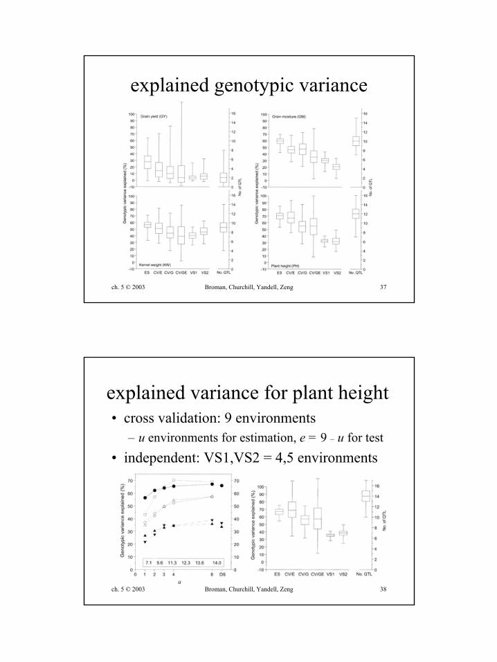
explained genotypic variance
ch. 5 © 2003 Broman, Churchill, Yandell, Zeng 38
explained variance for plant height• cross validation: 9 environments
– u environments for estimation, e = 9 – u for test• independent: VS1,VS2 = 4,5 environments
ch. 5 © 2003 Broman, Churchill, Yandell, Zeng 39
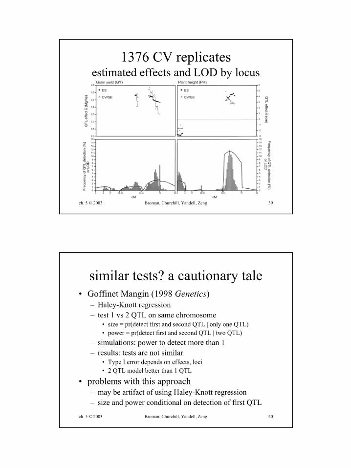
1376 CV replicatesestimated effects and LOD by locus
ch. 5 © 2003 Broman, Churchill, Yandell, Zeng 40
similar tests? a cautionary tale• Goffinet Mangin (1998 Genetics)
– Haley-Knott regression– test 1 vs 2 QTL on same chromosome
• size = pr(detect first and second QTL | only one QTL)• power = pr(detect first and second QTL | two QTL)
– simulations: power to detect more than 1– results: tests are not similar
• Type I error depends on effects, loci• 2 QTL model better than 1 QTL
• problems with this approach– may be artifact of using Haley-Knott regression– size and power conditional on detection of first QTL
ch. 5 © 2003 Broman, Churchill, Yandell, Zeng 41
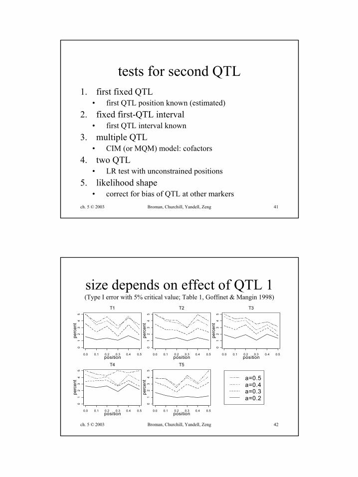
tests for second QTL1. first fixed QTL
• first QTL position known (estimated)2. fixed first-QTL interval
• first QTL interval known3. multiple QTL
• CIM (or MQM) model: cofactors4. two QTL
• LR test with unconstrained positions5. likelihood shape
• correct for bias of QTL at other markers
ch. 5 © 2003 Broman, Churchill, Yandell, Zeng 42
size depends on effect of QTL 1(Type I error with 5% critical value; Table 1, Goffinet & Mangin 1998)
0.0 0.1 0.2 0.3 0.4 0.5
01
23
45
position
perc
ent
T1
0.0 0.1 0.2 0.3 0.4 0.5
01
23
45
position
perc
ent
T2
0.0 0.1 0.2 0.3 0.4 0.5
01
23
45
position
perc
ent
T3
0.0 0.1 0.2 0.3 0.4 0.5
01
23
45
position
perc
ent
T4
0.0 0.1 0.2 0.3 0.4 0.5
01
23
45
position
perc
ent
T5
a=0.5a=0.4a=0.3a=0.2
ch. 5 © 2003 Broman, Churchill, Yandell, Zeng 43
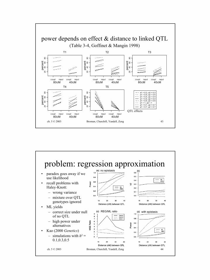
power depends on effect & distance to linked QTL(Table 3-4, Goffinet & Mangin 1998)
QTL effects
2040
6080
perc
ent
coupl repul coupl repul80cM 40cM
T1
2040
6080
perc
ent
coupl repul coupl repul80cM 40cM
T2
2040
6080
perc
ent
coupl repul coupl repul80cM 40cM
T3
2040
6080
perc
ent
coupl repul coupl repul80cM 40cM
T420
4060
80pe
rcen
t
coupl repul coupl repul80cM 40cM
T5
a1 = 0.3, a2 = 0.3a1 = 0.5, a2 = 0.5a1 = 0.4, a2 = 0.4a1 = 0.4, a2 = 0.4a1 = 0.5, a2 = 0.5a1 = 1, a2 = 1a1 = 0.7, a2 = 0.7a1 = 0.7, a2 = 0.7
ch. 5 © 2003 Broman, Churchill, Yandell, Zeng 44
problem: regression approximation• paradox goes away if we
use likelihood• recall problems with
Haley-Knott:– wrong variance– mixture over QTL
genotypes ignored• ML yields
– correct size under null of no QTL
– high power under alternatives
• Kao (2000 Genetics)– simulations with h2 =
0.1,0.3,0.5
with epistasis
no epistasis
REG/ML ratio


![course5 ||||| Linear Discriminant Analysis · A.B. Dufour 1 Fisher’s iris dataset The data were collected by Anderson [1] and used by Fisher [2] to formulate the linear discriminant](https://static.fdocuments.in/doc/165x107/5c386bc709d3f202338b6a97/course5-linear-discriminant-analysis-ab-dufour-1-fishers-iris-dataset.jpg)