1

Based on slides from the book

Database System Concepts, 5th Ed.

Query ProcessingQuery Processing

MichalisMichalis VazirgiannisVazirgiannishttp://www.dbhttp://www.db--net.aueb.gr/michalisnet.aueb.gr/michalis

11/200911/2009

13.2

Query ProcessingQuery Processing

Overview Measures of Query Cost Selection Operation Sorting Join Operation Other Operations Evaluation of Expressions

2

13.3

Basic Steps in Query ProcessingBasic Steps in Query Processing

1. Parsing and translation2. Optimization3. Evaluation

13.4

Basic Steps in Query Processing Basic Steps in Query Processing (Cont.)(Cont.)

Parsing and translation translate the query into its internal form. This is then translated into

relational algebra. Parser checks syntax, verifies relations

Evaluation The query-execution engine takes a query-evaluation plan, executes

that plan, and returns the answers to the query.

3

13.5

Basic Steps in Query Processing : Basic Steps in Query Processing : OptimizationOptimization

A relational algebra expression may have many equivalent expressions

E.g., balance2500(balance(account)) is equivalent to balance(balance2500(account))

Each relational algebra operation can be evaluated using one of several different algorithms Correspondingly, a relational-algebra expression can be evaluated in

many ways. Annotated expression specifying detailed evaluation strategy is called an

evaluation-plan. E.g., can use an index on balance to find accounts with balance < 2500, or can perform complete relation scan and discard accounts with

balance 2500

13.6

Basic Steps: Optimization (Cont.)Basic Steps: Optimization (Cont.)

Query Optimization: Amongst all equivalent evaluation plans choose the one with lowest cost. Cost is estimated using statistical information from the

database catalog e.g. number of tuples in each relation, size of tuples, etc.

Here we study How to measure query costs Algorithms for evaluating relational algebra operations How to combine algorithms for individual operations in order to

evaluate a complete expression Remains

how to optimize queries, that is, how to find an evaluation planwith lowest estimated cost

4

13.7

Measures of Query CostMeasures of Query Cost

Cost is generally measured as total elapsed time for answering query Many factors contribute to time cost

disk accesses, CPU, or even network communication Typically disk access is the predominant cost, and is also

relatively easy to estimate. Measured by taking into account Number of seeks * average-seek-cost Number of blocks read * average-block-read-cost Number of blocks written * average-block-write-cost

Cost to write a block is greater than cost to read a block – data is read back after being written to ensure that

the write was successful

13.8

Measures of Query Cost (Cont.)Measures of Query Cost (Cont.)

For simplicity we just use the number of block transfers from disk and the number of seeks as the cost measures tT – time to transfer one block tS – time for one seek Cost for b block transfers plus S seeks

b * tT + S * tS We ignore CPU costs for simplicity

Real systems do take CPU cost into account We do not include cost to writing output to disk in our cost formulae Several algorithms can reduce disk IO by using extra buffer space

Amount of real memory available to buffer depends on other concurrent queries and OS processes, known only during executionWe often use worst case estimates, assuming only the minimum

amount of memory needed for the operation is available Required data may be buffer resident already, avoiding disk I/O

But hard to take into account for cost estimation

5

13.9

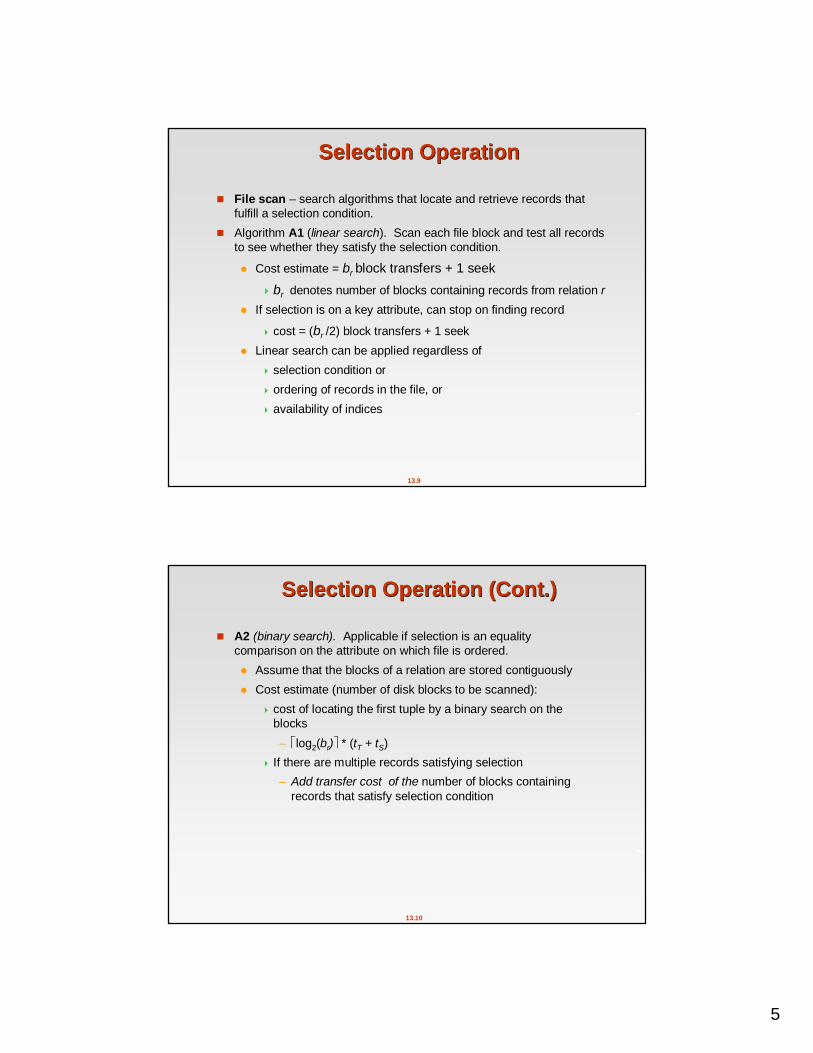
Selection OperationSelection Operation

File scan – search algorithms that locate and retrieve records that fulfill a selection condition.

Algorithm A1 (linear search). Scan each file block and test all records to see whether they satisfy the selection condition.

Cost estimate = br block transfers + 1 seekbr denotes number of blocks containing records from relation r

If selection is on a key attribute, can stop on finding record

cost = (br /2) block transfers + 1 seek Linear search can be applied regardless of

selection condition or ordering of records in the file, or availability of indices

13.10

Selection Operation (Cont.)Selection Operation (Cont.)

A2 (binary search). Applicable if selection is an equality comparison on the attribute on which file is ordered. Assume that the blocks of a relation are stored contiguously Cost estimate (number of disk blocks to be scanned):

cost of locating the first tuple by a binary search on the blocks– log2(br) * (tT + tS)

If there are multiple records satisfying selection– Add transfer cost of the number of blocks containing

records that satisfy selection condition

6

13.11

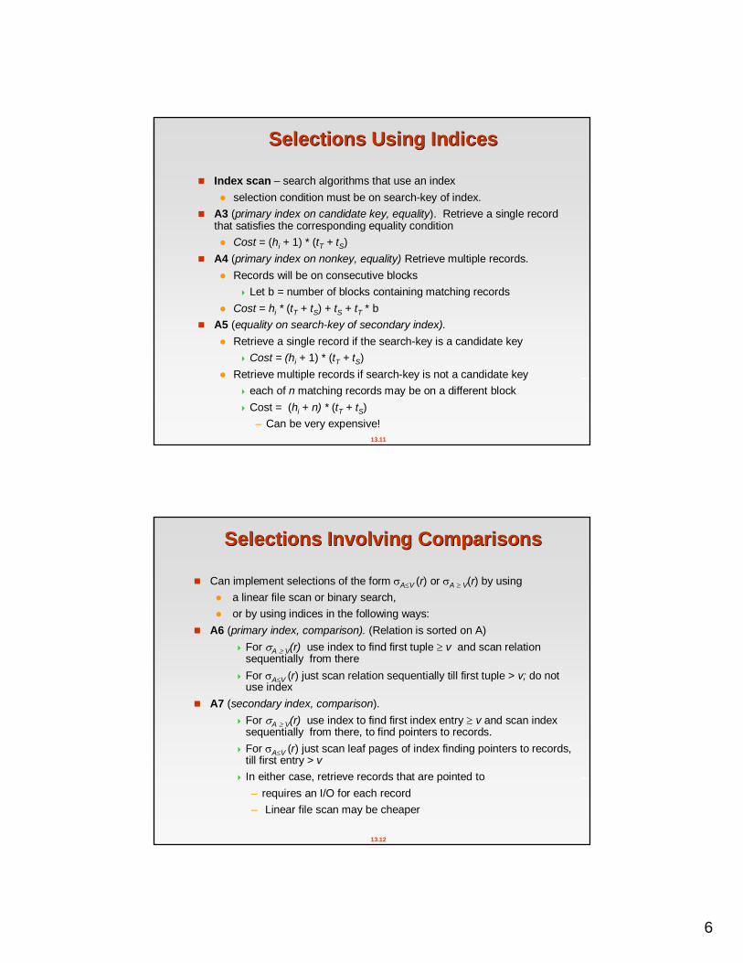
Selections Using IndicesSelections Using Indices

Index scan – search algorithms that use an index selection condition must be on search-key of index.

A3 (primary index on candidate key, equality). Retrieve a single record that satisfies the corresponding equality condition Cost = (hi + 1) * (tT + tS)

A4 (primary index on nonkey, equality) Retrieve multiple records. Records will be on consecutive blocks

Let b = number of blocks containing matching records Cost = hi * (tT + tS) + tS + tT * b

A5 (equality on search-key of secondary index). Retrieve a single record if the search-key is a candidate key

Cost = (hi + 1) * (tT + tS) Retrieve multiple records if search-key is not a candidate key

each of n matching records may be on a different block Cost = (hi + n) * (tT + tS)

– Can be very expensive!

13.12

Selections Involving ComparisonsSelections Involving Comparisons

Can implement selections of the form AV (r) or A V(r) by using a linear file scan or binary search, or by using indices in the following ways:

A6 (primary index, comparison). (Relation is sorted on A) For A V(r) use index to find first tuple v and scan relation

sequentially from there For AV (r) just scan relation sequentially till first tuple > v; do not

use index A7 (secondary index, comparison).

For A V(r) use index to find first index entry v and scan index sequentially from there, to find pointers to records.

For AV (r) just scan leaf pages of index finding pointers to records, till first entry > v

In either case, retrieve records that are pointed to– requires an I/O for each record– Linear file scan may be cheaper

7

13.13

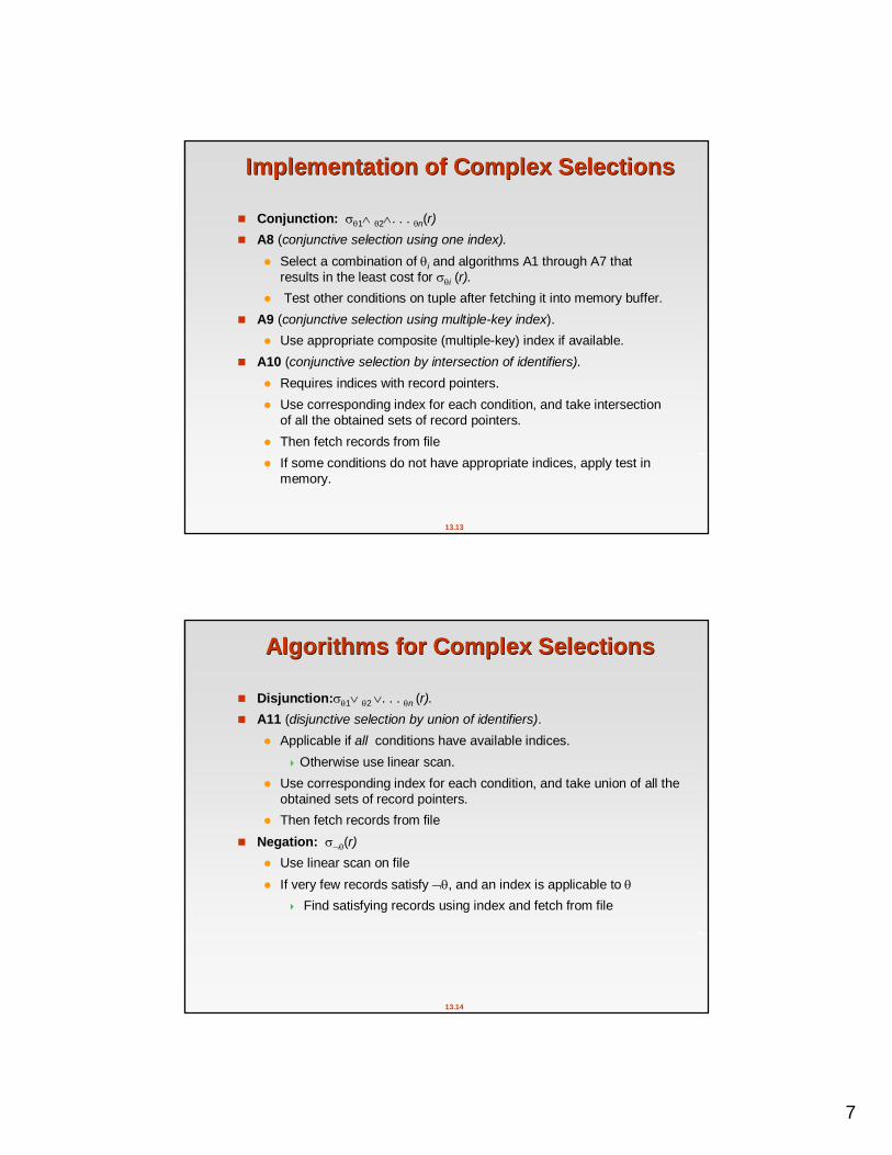
Implementation of Complex SelectionsImplementation of Complex Selections

Conjunction: 1 2. . . n(r) A8 (conjunctive selection using one index).

Select a combination of i and algorithms A1 through A7 that results in the least cost for i (r).

Test other conditions on tuple after fetching it into memory buffer. A9 (conjunctive selection using multiple-key index).

Use appropriate composite (multiple-key) index if available. A10 (conjunctive selection by intersection of identifiers).

Requires indices with record pointers. Use corresponding index for each condition, and take intersection

of all the obtained sets of record pointers. Then fetch records from file If some conditions do not have appropriate indices, apply test in

memory.

13.14

Algorithms for Complex SelectionsAlgorithms for Complex Selections

Disjunction:1 2 . . . n (r). A11 (disjunctive selection by union of identifiers).

Applicable if all conditions have available indices. Otherwise use linear scan.

Use corresponding index for each condition, and take union of all the obtained sets of record pointers.

Then fetch records from file Negation: (r)

Use linear scan on file If very few records satisfy , and an index is applicable to

Find satisfying records using index and fetch from file

8

13.15

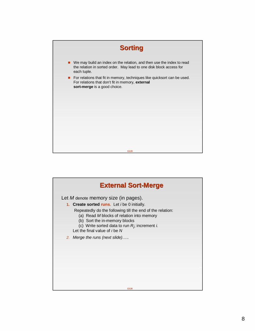
SortingSorting

We may build an index on the relation, and then use the index to read the relation in sorted order. May lead to one disk block access for each tuple.

For relations that fit in memory, techniques like quicksort can be used. For relations that don’t fit in memory, external sort-merge is a good choice.

13.16

External SortExternal Sort--MergeMerge

1. Create sorted runs. Let i be 0 initially.Repeatedly do the following till the end of the relation:

(a) Read M blocks of relation into memory(b) Sort the in-memory blocks(c) Write sorted data to run Ri; increment i.

Let the final value of i be N2. Merge the runs (next slide)…..

Let M denote memory size (in pages).

9

13.17

External SortExternal Sort--Merge (Cont.)Merge (Cont.)

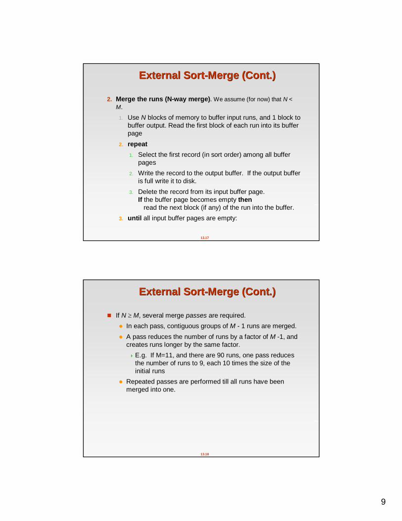
2. Merge the runs (N-way merge). We assume (for now) that N < M.

1. Use N blocks of memory to buffer input runs, and 1 block to buffer output. Read the first block of each run into its buffer page

2. repeat1. Select the first record (in sort order) among all buffer

pages2. Write the record to the output buffer. If the output buffer

is full write it to disk.3. Delete the record from its input buffer page.

If the buffer page becomes empty thenread the next block (if any) of the run into the buffer.

3. until all input buffer pages are empty:

13.18

External SortExternal Sort--Merge (Cont.)Merge (Cont.)

If N M, several merge passes are required. In each pass, contiguous groups of M - 1 runs are merged. A pass reduces the number of runs by a factor of M -1, and

creates runs longer by the same factor. E.g. If M=11, and there are 90 runs, one pass reduces

the number of runs to 9, each 10 times the size of the initial runs

Repeated passes are performed till all runs have been merged into one.

10

13.19

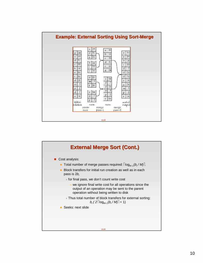
Example: External Sorting Using SortExample: External Sorting Using Sort--MergeMerge

13.20

External Merge Sort (Cont.)External Merge Sort (Cont.)

Cost analysis: Total number of merge passes required: logM–1(br / M). Block transfers for initial run creation as well as in each

pass is 2br

for final pass, we don’t count write cost – we ignore final write cost for all operations since the

output of an operation may be sent to the parent operation without being written to disk

Thus total number of block transfers for external sorting:br ( 2 logM–1(br / M) + 1)

Seeks: next slide

11

13.21

External Merge Sort (Cont.)External Merge Sort (Cont.)

Cost of seeks During run generation: one seek to read each run and one seek to

write each run 2 br / M

During the merge phase

Buffer size: bb (read/write bb blocks at a time)

Need 2 br / bb seeks for each merge pass – except the final one which does not require a write

Total number of seeks:2 br / M + br / bb (2 logM–1(br / M) -1)

13.22

Join OperationJoin Operation

Several different algorithms to implement joins Nested-loop join Block nested-loop join Indexed nested-loop join Merge-join Hash-join

Choice based on cost estimate Examples use the following information

Number of records of customer: 10,000 depositor: 5000 Number of blocks of customer: 400 depositor: 100

12

13.23

NestedNested--Loop JoinLoop Join

To compute the theta join r sfor each tuple tr in r do beginfor each tuple ts in s do begin

test pair (tr,ts) to see if they satisfy the join condition if they do, add tr • ts to the result.

endend

r is called the outer relation and s the inner relation of the join. Requires no indices and can be used with any kind of join condition. Expensive since it examines every pair of tuples in the two relations.

13.24

NestedNested--Loop Join (Cont.)Loop Join (Cont.)

In the worst case, if there is enough memory only to hold one block of each relation, the estimated cost is

nr bs + brblock transfers, plus

nr + brseeks

If the smaller relation fits entirely in memory, use that as the inner relation.

Reduces cost to br + bs block transfers and 2 seeks Assuming worst case memory availability cost estimate is

with depositor as outer relation:

5000 400 + 100 = 2,000,100 block transfers, 5000 + 100 = 5100 seeks

with customer as the outer relation

10000 100 + 400 = 1,000,400 block transfers and 10,400 seeks If smaller relation (depositor) fits entirely in memory, the cost estimate will be 500

block transfers. Block nested-loops algorithm (next slide) is preferable.

13

13.25

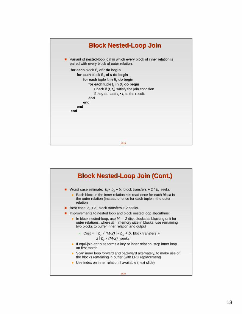
Block NestedBlock Nested--Loop JoinLoop Join

Variant of nested-loop join in which every block of inner relation is paired with every block of outer relation.

for each block Br of r do beginfor each block Bs of s do begin

for each tuple tr in Br do beginfor each tuple ts in Bs do begin

Check if (tr,ts) satisfy the join condition if they do, add tr • ts to the result.

endend

endend

13.26

Block NestedBlock Nested--Loop Join (Cont.)Loop Join (Cont.)

Worst case estimate: br bs + br block transfers + 2 * br seeks Each block in the inner relation s is read once for each block in

the outer relation (instead of once for each tuple in the outer relation

Best case: br + bs block transfers + 2 seeks. Improvements to nested loop and block nested loop algorithms:

In block nested-loop, use M — 2 disk blocks as blocking unit for outer relations, where M = memory size in blocks; use remaining two blocks to buffer inner relation and output

Cost = br / (M-2) bs + br block transfers +2 br / (M-2) seeks

If equi-join attribute forms a key or inner relation, stop inner loop on first match

Scan inner loop forward and backward alternately, to make use ofthe blocks remaining in buffer (with LRU replacement)

Use index on inner relation if available (next slide)

14

13.27

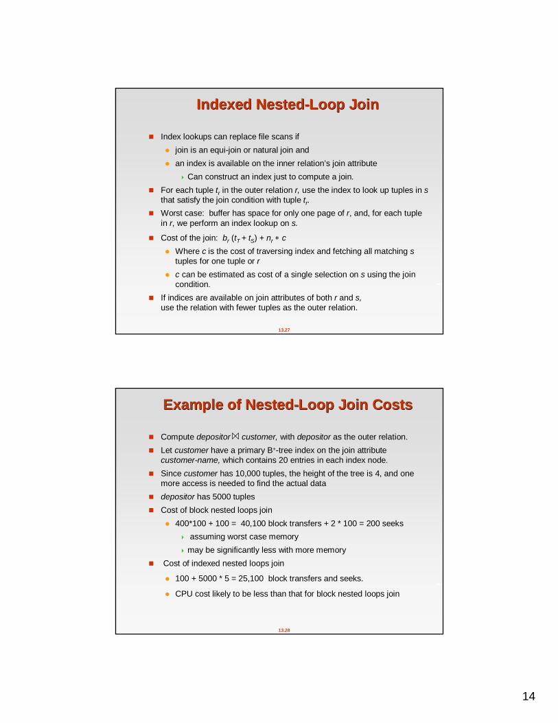
Indexed NestedIndexed Nested--Loop JoinLoop Join

Index lookups can replace file scans if join is an equi-join or natural join and an index is available on the inner relation’s join attribute

Can construct an index just to compute a join. For each tuple tr in the outer relation r, use the index to look up tuples in s

that satisfy the join condition with tuple tr. Worst case: buffer has space for only one page of r, and, for each tuple

in r, we perform an index lookup on s.

Cost of the join: br (tT + tS) + nr c Where c is the cost of traversing index and fetching all matching s

tuples for one tuple or r c can be estimated as cost of a single selection on s using the join

condition. If indices are available on join attributes of both r and s,

use the relation with fewer tuples as the outer relation.

13.28

Example of NestedExample of Nested--Loop Join CostsLoop Join Costs

Compute depositor customer, with depositor as the outer relation. Let customer have a primary B+-tree index on the join attribute

customer-name, which contains 20 entries in each index node. Since customer has 10,000 tuples, the height of the tree is 4, and one

more access is needed to find the actual data depositor has 5000 tuples Cost of block nested loops join

400*100 + 100 = 40,100 block transfers + 2 * 100 = 200 seeks assuming worst case memory may be significantly less with more memory

Cost of indexed nested loops join

100 + 5000 * 5 = 25,100 block transfers and seeks.

CPU cost likely to be less than that for block nested loops join

15

13.29

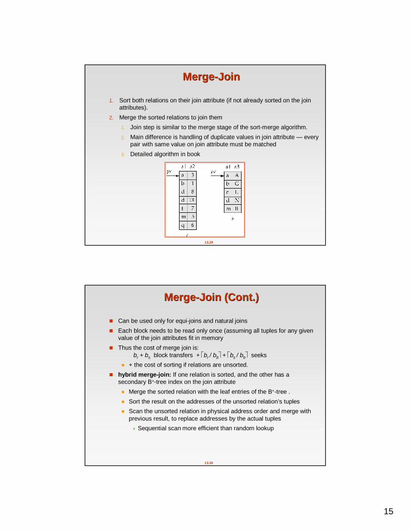
MergeMerge--JoinJoin

1. Sort both relations on their join attribute (if not already sorted on the join attributes).

2. Merge the sorted relations to join them1. Join step is similar to the merge stage of the sort-merge algorithm. 2. Main difference is handling of duplicate values in join attribute — every

pair with same value on join attribute must be matched3. Detailed algorithm in book

13.30

MergeMerge--Join (Cont.)Join (Cont.)

Can be used only for equi-joins and natural joins Each block needs to be read only once (assuming all tuples for any given

value of the join attributes fit in memory Thus the cost of merge join is:

br + bs block transfers + br / bb + bs / bb seeks + the cost of sorting if relations are unsorted.

hybrid merge-join: If one relation is sorted, and the other has a secondary B+-tree index on the join attribute Merge the sorted relation with the leaf entries of the B+-tree . Sort the result on the addresses of the unsorted relation’s tuples Scan the unsorted relation in physical address order and merge with

previous result, to replace addresses by the actual tuples Sequential scan more efficient than random lookup

16

13.31

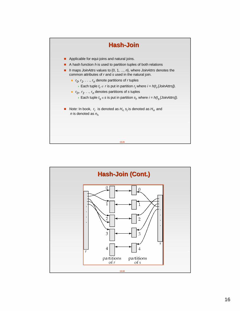
HashHash--JoinJoin

Applicable for equi-joins and natural joins. A hash function h is used to partition tuples of both relations h maps JoinAttrs values to {0, 1, ..., n}, where JoinAttrs denotes the

common attributes of r and s used in the natural join. r0, r1, . . ., rn denote partitions of r tuples

Each tuple tr r is put in partition ri where i = h(tr [JoinAttrs]). r0,, r1. . ., rn denotes partitions of s tuples

Each tuple ts s is put in partition si, where i = h(ts [JoinAttrs]).

Note: In book, ri is denoted as Hri, si is denoted as Hsi andn is denoted as nh.

13.32

HashHash--Join (Cont.)Join (Cont.)

17

13.33

HashHash--Join (Cont.)Join (Cont.)

r tuples in ri need only to be compared with s tuples in si Need not be compared with s tuples in any other partition, since: an r tuple and an s tuple that satisfy the join condition will

have the same value for the join attributes. If that value is hashed to some value i, the r tuple has to be in

ri and the s tuple in si.

13.34

HashHash--Join AlgorithmJoin Algorithm

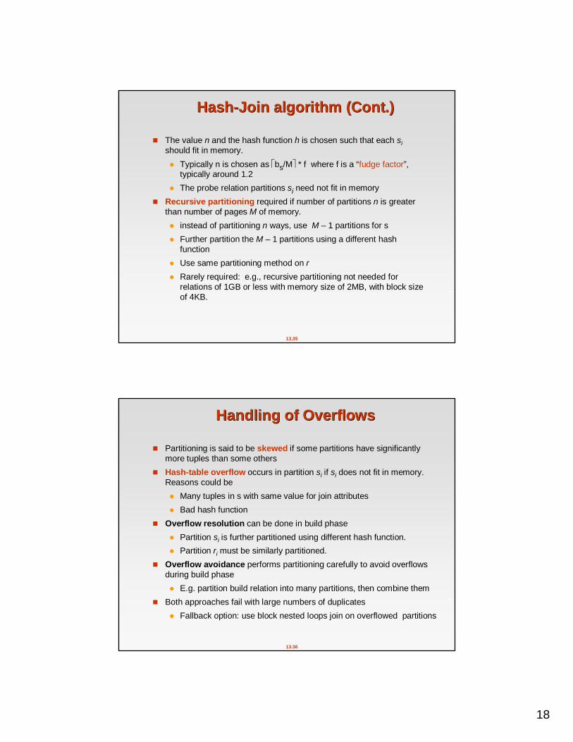
1. Partition the relation s using hashing function h. When partitioning a relation, one block of memory is reserved as the output buffer for each partition.

2. Partition r similarly.3. For each i:

(a) Load si into memory and build an in-memory hash index on it using the join attribute. This hash index uses a different hashfunction than the earlier one h.

(b) Read the tuples in ri from the disk one by one. For each tuple tr locate each matching tuple ts in si using the in-memory hash index. Output the concatenation of their attributes.

The hash-join of r and s is computed as follows.

Relation s is called the build input and r is called the probe input.

18

13.35

HashHash--Join algorithm (Cont.)Join algorithm (Cont.)

The value n and the hash function h is chosen such that each sishould fit in memory. Typically n is chosen as bs/M * f where f is a “fudge factor”,

typically around 1.2 The probe relation partitions si need not fit in memory

Recursive partitioning required if number of partitions n is greater than number of pages M of memory. instead of partitioning n ways, use M – 1 partitions for s Further partition the M – 1 partitions using a different hash

function Use same partitioning method on r Rarely required: e.g., recursive partitioning not needed for

relations of 1GB or less with memory size of 2MB, with block size of 4KB.

13.36

Handling of OverflowsHandling of Overflows

Partitioning is said to be skewed if some partitions have significantly more tuples than some others

Hash-table overflow occurs in partition si if si does not fit in memory. Reasons could be Many tuples in s with same value for join attributes Bad hash function

Overflow resolution can be done in build phase Partition si is further partitioned using different hash function. Partition ri must be similarly partitioned.

Overflow avoidance performs partitioning carefully to avoid overflows during build phase E.g. partition build relation into many partitions, then combine them

Both approaches fail with large numbers of duplicates Fallback option: use block nested loops join on overflowed partitions

19

13.37

Cost of HashCost of Hash--JoinJoin

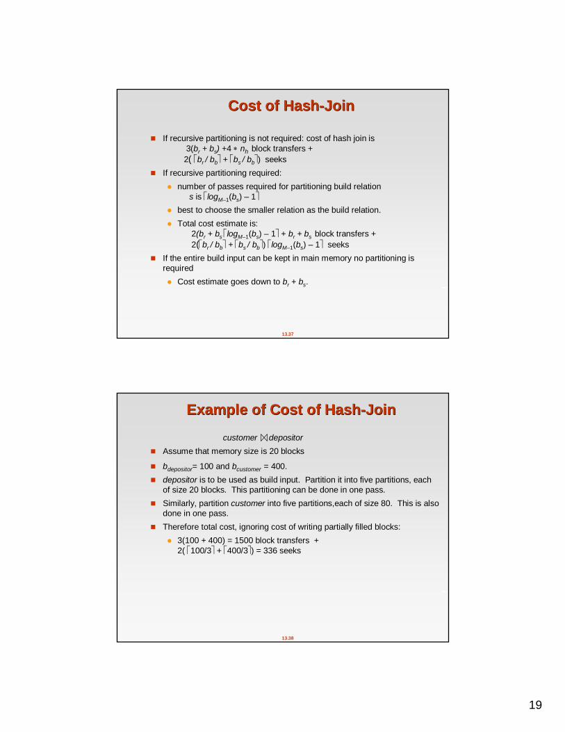
If recursive partitioning is not required: cost of hash join is3(br + bs) +4 nh block transfers +2( br / bb + bs / bb) seeks

If recursive partitioning required: number of passes required for partitioning build relation

s is logM–1(bs) – 1 best to choose the smaller relation as the build relation. Total cost estimate is:

2(br + bs logM–1(bs) – 1 + br + bs block transfers + 2(br / bb + bs / bb) logM–1(bs) – 1 seeks

If the entire build input can be kept in main memory no partitioning is required Cost estimate goes down to br + bs.

13.38

Example of Cost of HashExample of Cost of Hash--JoinJoin

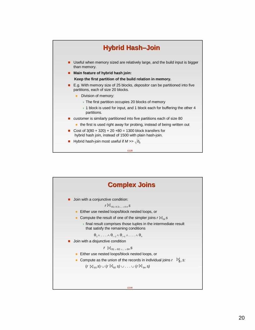
Assume that memory size is 20 blocks

bdepositor= 100 and bcustomer = 400. depositor is to be used as build input. Partition it into five partitions, each

of size 20 blocks. This partitioning can be done in one pass. Similarly, partition customer into five partitions,each of size 80. This is also

done in one pass. Therefore total cost, ignoring cost of writing partially filled blocks:

3(100 + 400) = 1500 block transfers +2( 100/3 + 400/3) = 336 seeks

customer depositor

20

13.39

Hybrid HashHybrid Hash––JoinJoin

Useful when memory sized are relatively large, and the build input is bigger than memory.

Main feature of hybrid hash join:Keep the first partition of the build relation in memory.

E.g. With memory size of 25 blocks, depositor can be partitioned into five partitions, each of size 20 blocks. Division of memory:

The first partition occupies 20 blocks of memory 1 block is used for input, and 1 block each for buffering the other 4

partitions. customer is similarly partitioned into five partitions each of size 80

the first is used right away for probing, instead of being written out Cost of 3(80 + 320) + 20 +80 = 1300 block transfers for

hybrid hash join, instead of 1500 with plain hash-join. Hybrid hash-join most useful if M >> sb

13.40

Complex JoinsComplex Joins

Join with a conjunctive condition:r 1 2... n s

Either use nested loops/block nested loops, or Compute the result of one of the simpler joins r i s

final result comprises those tuples in the intermediate result that satisfy the remaining conditions

1 . . . i –1 i +1 . . . n

Join with a disjunctive condition

r 1 2 ... n s Either use nested loops/block nested loops, or Compute as the union of the records in individual joins r i s:

(r 1 s) (r 2 s) . . . (r n s)

21

13.41

Other OperationsOther Operations

Duplicate elimination can be implemented via hashing or sorting. On sorting duplicates will come adjacent to each other, and all but

one set of duplicates can be deleted. Optimization: duplicates can be deleted during run generation as

well as at intermediate merge steps in external sort-merge. Hashing is similar – duplicates will come into the same bucket.

Projection: perform projection on each tuple followed by duplicate elimination.

13.42

Other Operations : AggregationOther Operations : Aggregation

Aggregation can be implemented in a manner similar to duplicate elimination. Sorting or hashing can be used to bring tuples in the same group

together, and then the aggregate functions can be applied on each group.

Optimization: combine tuples in the same group during run generation and intermediate merges, by computing partial aggregate values For count, min, max, sum: keep aggregate values on tuples

found so far in the group. – When combining partial aggregate for count, add up the

aggregates For avg, keep sum and count, and divide sum by count at the

end

22

13.43

Other Operations : Set OperationsOther Operations : Set Operations

Set operations (, and ): can either use variant of merge-join after sorting, or variant of hash-join.

E.g., Set operations using hashing:1. Partition both relations using the same hash function2. Process each partition i as follows.

1. Using a different hashing function, build an in-memory hash index on ri.

2. Process si as follows r s:

1. Add tuples in si to the hash index if they are not already in it. 2. At end of si add the tuples in the hash index to the result.

r s: 1. output tuples in si to the result if they are already there in the

hash index r – s:

1. for each tuple in si, if it is there in the hash index, delete it from the index.

2. At end of si add remaining tuples in the hash index to the result.

13.44

Other Operations : Outer JoinOther Operations : Outer Join

Outer join can be computed either as A join followed by addition of null-padded non-participating tuples. by modifying the join algorithms.

Modifying merge join to compute r s In r s, non participating tuples are those in r – R(r s) Modify merge-join to compute r s: During merging, for every

tuple tr from r that do not match any tuple in s, output tr padded with nulls.

Right outer-join and full outer-join can be computed similarly. Modifying hash join to compute r s

If r is probe relation, output non-matching r tuples padded with nulls If r is build relation, when probing keep track of which

r tuples matched s tuples. At end of si output non-matched r tuples padded with nulls

23

13.45

Evaluation of ExpressionsEvaluation of Expressions

So far: we have seen algorithms for individual operations Alternatives for evaluating an entire expression tree

Materialization: generate results of an expression whose inputs are relations or are already computed, materialize (store) it on disk. Repeat.

Pipelining: pass on tuples to parent operations even as an operation is being executed

We study above alternatives in more detail

13.46

MaterializationMaterialization

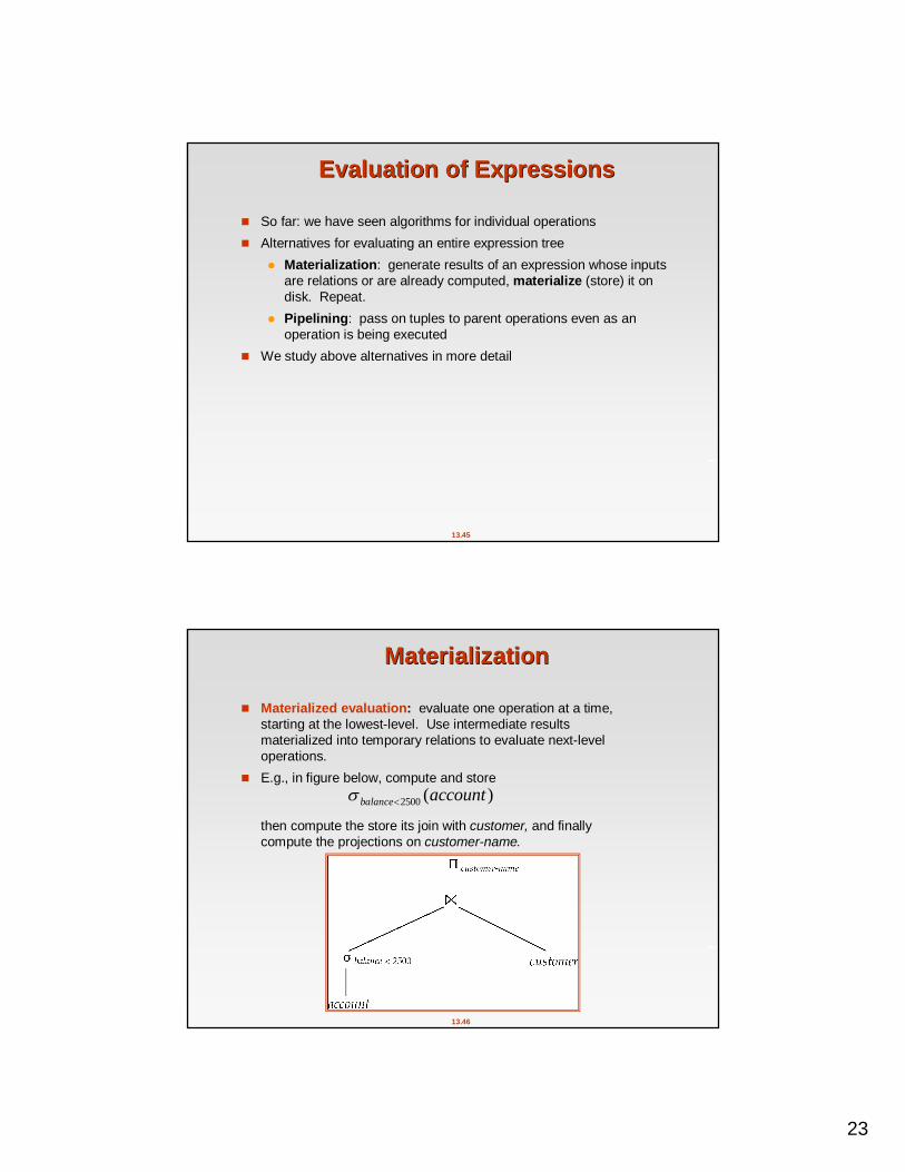
Materialized evaluation: evaluate one operation at a time, starting at the lowest-level. Use intermediate results materialized into temporary relations to evaluate next-level operations.

E.g., in figure below, compute and store

then compute the store its join with customer, and finally compute the projections on customer-name.

)(2500 accountbalance

24

13.47

Materialization (Cont.)Materialization (Cont.)

Materialized evaluation is always applicable Cost of writing results to disk and reading them back can be quite high

Our cost formulas for operations ignore cost of writing results to disk, soOverall cost = Sum of costs of individual operations +

cost of writing intermediate results to disk Double buffering: use two output buffers for each operation, when one

is full write it to disk while the other is getting filled Allows overlap of disk writes with computation and reduces

execution time

13.48

PipeliningPipelining

Pipelined evaluation : evaluate several operations simultaneously, passing the results of one operation on to the next.

E.g., in previous expression tree, don’t store result of

instead, pass tuples directly to the join.. Similarly, don’t store result of join, pass tuples directly to projection.

Much cheaper than materialization: no need to store a temporary relation to disk.

Pipelining may not always be possible – e.g., sort, hash-join. For pipelining to be effective, use evaluation algorithms that generate

output tuples even as tuples are received for inputs to the operation. Pipelines can be executed in two ways: demand driven and producer

driven

)(2500 accountbalance

25

13.49

Pipelining (Cont.)Pipelining (Cont.)

In demand driven or lazy evaluation system repeatedly requests next tuple from top level operation Each operation requests next tuple from children operations as

required, in order to output its next tuple In between calls, operation has to maintain “state” so it knows what

to return next In producer-driven or eager pipelining

Operators produce tuples eagerly and pass them up to their parents Buffer maintained between operators, child puts tuples in buffer,

parent removes tuples from buffer if buffer is full, child waits till there is space in the buffer, and then

generates more tuples System schedules operations that have space in output buffer and

can process more input tuples Alternative name: pull and push models of pipelining

13.50

Pipelining (Cont.)Pipelining (Cont.)

Implementation of demand-driven pipelining Each operation is implemented as an iterator implementing the

following operations open()

– E.g. file scan: initialize file scan» state: pointer to beginning of file

– E.g.merge join: sort relations;» state: pointers to beginning of sorted relations

next()– E.g. for file scan: Output next tuple, and advance and store

file pointer– E.g. for merge join: continue with merge from earlier state

till next output tuple is found. Save pointers as iterator state.

close()

26

13.51

Evaluation Algorithms for PipeliningEvaluation Algorithms for Pipelining

Some algorithms are not able to output results even as they get input tuples E.g. merge join, or hash join intermediate results written to disk and then read back

Algorithm variants to generate (at least some) results on the fly, as input tuples are read in E.g. hybrid hash join generates output tuples even as probe relation

tuples in the in-memory partition (partition 0) are read in Pipelined join technique: Hybrid hash join, modified to buffer

partition 0 tuples of both relations in-memory, reading them as they become available, and output results of any matches between partition 0 tuplesWhen a new r0 tuple is found, match it with existing s0 tuples,

output matches, and save it in r0 Symmetrically for s0 tuples

Based on slides from the book

Database System Concepts, 5th Ed.

End of ChapterEnd of Chapter

27

13.53

Figure 13.2Figure 13.2

13.54

Complex JoinsComplex Joins

Join involving three relations: loan depositor customer Strategy 1. Compute depositor customer; use result to compute

loan (depositor customer) Strategy 2. Computer loan depositor first, and then join the

result with customer. Strategy 3. Perform the pair of joins at once. Build and index on

loan for loan-number, and on customer for customer-name. For each tuple t in depositor, look up the corresponding tuples

in customer and the corresponding tuples in loan. Each tuple of deposit is examined exactly once.

Strategy 3 combines two operations into one special-purpose operation that is more efficient than implementing two joins of two relations.