5. PLUME OR JET MODELS IN HGSYSTEM · HGSYSTEM Technical Reference Manual 5-2 5. PLUME OR JET...
90
HGSYSTEM Technical Reference Manual 5-1 5. PLUME OR JET MODELS IN HGSYSTEM CONTENTS 5. PLUME OR JET MODELS IN HGSYSTEM 5-1 5.A. THE AEROPLUME MODEL 5-3 5.A.1. Introduction 5-3 5.A.2. The AEROPLUME code 5-3 5.A.3. Summary of the aerosol algorithm 5-4 5.A.4. The reservoir state calculation 5-6 5.A.5. Calculation of post-flash conditions 5-7 5.A.6. Discharge rate specification 5-13 5.A.7. Plume development model 5-16 5.A.8. References 5-19 5.A.9. Notation 5-20 5.B. DEVELOPMENT OF PLUME AND JET RELEASE MODELS 5-22 5.B.1. Introduction 5-22 5.B.2. The Stages of Plume Development 5-23 5.B.3. Control Volume Analysis: Basic equations of Motion 5-26 5.B.4. External flashing; Flow Establishment; Gaussian profiles 5-31 5.B.5. The Airborne Plume: geometry and shear entrainment 5-34 5.B.6. The Touchdown and Slumped Plume 5-37 5.B.7. Closure Assumptions for the 'Top-Hat' Model 5-40 5.B.8. The Entrainment Function 5-47 5.B.9. The atmosphere model. 5-54 5.B.10. Plume cross-sectional over-lap: curvature limited entrainment 5-54 5.B.11. The HGSYSTEM plume models: algorithmic structure. 5-57 5.B.12. Validation studies, entrainment formulae 5-57 5.B.13. Comparison with models of Wheatley, Raj and Morris, and Havens 5-60 5.B.14. References 5-64
Transcript of 5. PLUME OR JET MODELS IN HGSYSTEM · HGSYSTEM Technical Reference Manual 5-2 5. PLUME OR JET...

HGSYSTEM Technical Reference Manual
5-1
5. PLUME OR JET MODELS IN HGSYSTEM
CONTENTS
5. PLUME OR JET MODELS IN HGSYSTEM 5-1
5.A. THE AEROPLUME MODEL 5-3
5.A.1. Introduction 5-3
5.A.2. The AEROPLUME code 5-3
5.A.3. Summary of the aerosol algorithm 5-4
5.A.4. The reservoir state calculation 5-6
5.A.5. Calculation of post-flash conditions 5-7
5.A.6. Discharge rate specification 5-13
5.A.7. Plume development model 5-16
5.A.8. References 5-19
5.A.9. Notation 5-20
5.B. DEVELOPMENT OF PLUME AND JET RELEASE MODELS 5-22
5.B.1. Introduction 5-22
5.B.2. The Stages of Plume Development 5-23
5.B.3. Control Volume Analysis: Basic equations of Motion 5-26
5.B.4. External flashing; Flow Establishment; Gaussian profiles 5-31
5.B.5. The Airborne Plume: geometry and shear entrainment 5-34
5.B.6. The Touchdown and Slumped Plume 5-37
5.B.7. Closure Assumptions for the 'Top-Hat' Model 5-40
5.B.8. The Entrainment Function 5-47
5.B.9. The atmosphere model. 5-54
5.B.10. Plume cross-sectional over-lap: curvature limited entrainment 5-54
5.B.11. The HGSYSTEM plume models: algorithmic structure. 5-57
5.B.12. Validation studies, entrainment formulae 5-57
5.B.13. Comparison with models of Wheatley, Raj and Morris, and Havens 5-60
5.B.14. References 5-64

HGSYSTEM Technical Reference Manual
5-2
5. PLUME OR JET MODELS IN HGSYSTEM
The HGSYSTEM package contains two models to describe the dispersion of a jet release from
a pressurised vessel. AEROPLUME can be applied to non-reactive, multi-compound two-
phase jets and HFPLUME describes jet dispersion using the full hydrogen fluoride (HF)
chemistry and thermodynamics. The two thermodynamic models used, are discussed in detail
in Chapter 2. Chapter 2.A. describes the thermodynamics as used in AEROPLUME and
Chapter 2.B. describes the hydrogen fluoride thermodynamic model as used in HFPLUME.
AEROPLUME and HFPLUME both have a similar discharge model to estimate release
(discharge) rates from a given pressurised vessel.
In the new HGSYSTEM version 3.0, AEROPLUME replaces the PLUME model which was
available in the first public release, HGSYSTEM version 1.0 (also called NOV90 version).
PLUME could only deal with ideal gas releases.
In Chapter 5.A, the AEROPLUME implementation in HGSYSTEM version 3.0 is discussed in
more detail.
AEROPLUME, HFPLUME and the old PLUME model, all share the same basic plume
development description. This basic plume model is discussed in Chapter 5.B. In this chapter
also validation studies for the HGSYSTEM plume models are discussed.
The main difference between AEROPLUME and HFPLUME (and PLUME) is the
thermodynamic description of the released fluid. The way in which the thermodynamic
relations are solved is also different in AEROPLUME and HFPLUME. This is discussed in
Chapter 5.A., paragraph 5.A.7.
As HFPLUME is very similar to AEROPLUME, apart from the thermodynamics, there is no
separate discussion of HFPLUME in this Technical Reference Manual.

HGSYSTEM Technical Reference Manual
5-3
5.A. THE AEROPLUME MODEL
5.A.1. Introduction
The module in HGSYSTEM version 1.0 (or NOV90 version) describing steady-state
pressurised releases of a non-reactive pollutant, PLUME, has been updated considerably for
use in HGSYSTEM version 3.0, resulting in the newly named AEROPLUME model.
This chapter provides details about the implementation of the AEROPLUME (version 1.4)
module of HGSYSTEM version 3.0. AEROPLUME can be used to simulate the jet (plume)
development of a release, from a pressurised vessel or from a stack, of a mixture of several
non-reacting compounds, which can form one or more single or multi-compound aerosols.
AEROPLUME is in fact the result of combining the multi-compound, two-phase thermo-
dynamic model described in Chapter 2.A. with a PLUME (HFPLUME) jet description.
After a general introduction into the AEROPLUME code, the aerosol algorithms will be
summarised, then the reservoir and the post-flash calculations will be reviewed and finally a
summary of the equations describing the jet development will be given.
In Chapter 5B, the general plume or jet description developed for the old PLUME model, is
given. This chapter gives more details on the plume relations as discussed in paragraph 5.A.7
of the current Chapter 5.A.
Detailed information on AEROPLUME input parameters can be found in the AEROPLUME
chapter of the HGSYSTEM 3.0 User's Manual.
Please note that the HFPLUME model in HGSYSTEM is simply an HF-specific version of the
AEROPLUME model. The basic discharge model and jet description are very similar to the
one described in the current chapter. For this reason, HFPLUME will not be described
separately in this Technical Reference Manual. HFPLUME input parameters are described in
the HGSYSTEM 3.0 User's Manual.
5.A.2. The AEROPLUME code
Within the AEROPLUME code several main program blocks can be distinguished.
First there are the specific thermodynamic routines which contain the multi-compound aerosol
model. These routines calculate the plume thermodynamic variables, the reservoir state and
the post-flash or stack conditions. The structure is completely modular in the sense that the
HGSYSTEM Technical Reference Manual
5-4
thermodynamic routines are completely separated from the routines calculating the plume
development. The only communication is via the parameter lists.
The second main block consists of the routines to calculate the jet (plume) development. These
are basically the same routines as used in the old PLUME model (HGSYSTEM version 1.0)
and in HFPLUME. They contain, among other things, the entrainment models, the geometry
model and the plume integration routines which describe the position and composition (air
and pollutant) of the plume as it travels onward from its release point.
The original jet development description as used for the old PLUME model can be found in
Chapter 5B.
In the current chapter the specific AEROPLUME implementation is discussed.
Two of the solved variables are the plume enthalpy H and the total mass flow rate (pollutant
plus mixed-in air) &m (see paragraph 5.A.7). Together with the pollutant mass flow rate (or
discharge rate), which is a constant, these variables are communicated to the thermodynamic
routine in which the complete thermodynamic state of the plume at the current position is then
calculated. The plume density and temperature and the pollutant concentration are output from
the thermodynamic routine. Only the plume density is actually being used by the plume
integration routines as will be discussed in more detail in paragraph 5.A.7.
A third main block contains the routines describing the thermodynamic state of the ambient
atmosphere as a function of height, given the stability class and a set of reference values.
A last block that can be distinguished contains the input and output routines.
Because the thermodynamics is now built in a systematic, modular way, it should be a
straightforward task to replace the current thermodynamics model by another one if required.
Finally it should be noted that it is still possible to run AEROPLUME in the vapour-only
mode (i.e. the old PLUME model), but condensation of ambient water is now fully taken into
account.
5.A.3. Summary of the aerosol algorithm
A more detailed exposure of the HGSYSTEM multi-compound, two-phase aerosol model can
be found in Chapter 2. The formulation as given in this chapter is as used in HEGADAS and
HEGABOX. AEROPLUME uses a slightly different formulation as will be discussed below.

HGSYSTEM Technical Reference Manual
5-5
Consider a mixture of N chemical compounds which in principle can form M aerosols.
Aerosol β (β = 1, 2,..., M), when actually formed, will contain the compounds α where
α = nβ-1+1,..., nβ (0 = n0 < n1 < ... < nM = N). See Chapter 2 for more details.
Thus any combination of single compound and multi-compound aerosols is possible.
A slightly modified version of the general solution algorithm for the aerosol equations as
given in Chapter 2.A.
The set of equations, occurring in the innermost iteration loop of the aerosol algorithm, from
which the mole fraction liquid Lβ of each aerosol β that forms is calculated, is solved using the
non-linear algebraic equation solver NAESOL [1]. The solver proves to be very robust: the
solutions for the Lβ's are found without any convergence problems.
The modification made to the algorithm as proposed in Chapter 2, concerns the handling of
the singular point at T = 0° C (273.15 K) where a phase change of liquid water to ice takes
place, if any water is present in the mixture.
To prevent a discontinuity occurring in the enthalpy H at 0° C, because of the ice formation
term, a melting range [T1,T2] has been introduced, where T1 < 0° C and T2 > 0° C. Within this
melting range the enthalpy changes linearly from its value at T1 to its value at T2 and thus
effectively the sharp jump has been removed. This was necessary because during the jet
development calculations the former discontinuity gave rise to convergence problems of the
solver of the differential equations involved. In the present implementation T1 = - 0.15° C and
T2 = + 0.15° C .
When calculating the overall aerosol mixture density, in the original formulation (Chapter
2.A.), the volume of the liquid phase is neglected. Within a pressurised release context
however, this is no longer a valid simplification as liquid mole fractions can be high.
Therefore the overall mixture density ρ in AEROPLUME is calculated as follows:
ρ
ρα α
αα
=⋅
+ − ⋅ ⋅RSTUVW=
∑
M
M yL
R TP
l
l
( )1 0
1
N(1)
where M is the mixture molar mass, Mα the molar mass of compound α, yαl the molar
fraction within the mixture of the liquid phase of compound α, ραl is the liquid density of
compound α, L is the overall liquid mole fraction of the mixture, R0 the universal gas
constant, T the mixture temperature and P the mixture (vapour phase) pressure.

HGSYSTEM Technical Reference Manual
5-6
Of course the first term within the curly brackets is associated with the liquid volume and the
second term with the vapour volume, assuming ideal gas behaviour.
The mixture molar mass M is found from
M y M= ⋅∑ α αα=
N
1
(2)
where yα is the mixture mole fraction of compound α.
5.A.4. The reservoir state calculation
Within the context of two-phase fluid storage and discharge, it is important to emphasise that
the reservoir conditions being used should be representative of the fluid conditions in the
immediate neighbourhood of the discharge orifice. The aerosol model in fact uses a pseudo-
one-phase approach: liquid and vapour are assumed to be homogeneously distributed in terms
of the vapour-liquid ratios. Single liquid droplets can not be distinguished and a droplet size
distribution is not used.
For a given situation the user should realise that the location of the orifice can strongly
influence the liquid-vapour ratio of the discharged fluid. E.g. if in a reservoir filled with
propane half of the volume is occupied by liquid propane and the other half by propane
vapour, depending on the location of the discharge orifice either a pure liquid release or a pure
vapour release would occur. It is the user's responsibility to supply the correct reservoir
conditions. The code will give details on the reservoir state and on the post-flash state to
enable the user to check if the correct case is being simulated.
From the user-supplied reservoir conditions (temperature and pressure) and from the user-
supplied mixture composition (compound names and mole fractions) the equilibrium reservoir
state can be calculated using a simplified version of the aerosol algorithm as mentioned above.
The simplification lies in the fact that the temperature T is now given. Instead of a double
iteration loop to calculate T and the Lβ's, a single loop for the Lβ's only, is being used.
Again, the algorithm proves to be very robust.
When using the aerosol thermodynamics model, the user has the option not to specify the
reservoir pressure. In this case the AEROPLUME program will calculate the reservoir mixture
saturation pressure at the (user-supplied) reservoir temperature Tres using Raoult's law as
follows

HGSYSTEM Technical Reference Manual
5-7
P y P Tsat mix sat res, , ( )= ⋅=
∑ αα
α1
N
(3)
where yα is the mixture mole fraction of compound α and Psat,α(T) is the saturated vapour
pressure of compound α. It is assumed in (3) that the sum of the molar fractions yα is 1.
The reservoir pressure is then set to this saturation pressure.
It is thus assumed that all compounds α are in the liquid-only state. If this assumption is
reasonable, then relation (3) will give a reasonable reservoir pressure.
5.A.5. Calculation of post-flash conditions
To initiate the actual jet development calculations, the initial post-flash jet properties are
calculated from the reservoir state and the user-supplied orifice diameter and discharge mass
flow rate. These properties are: Uflash, Hflash and Dflash, which are velocity, enthalpy and diameter
of the jet respectively.
From these the thermodynamic (aerosol) model gives values for the temperature Tflash and
density ρflash.
The pollutant concentration is taken to be 100 % as air entrainment is assumed to be
negligible during this initial flashing process.
The calculation consists of two parts. First an adiabatic and frictionless acceleration of the
(stagnant) reservoir fluid to a point just outside the orifice is assumed. Vapour and liquid
velocities are assumed equal. There is no inter-phase heat exchange.
The maximum possible mass flow rate is calculated using choked flow relations and some
vapour is assumed to be present in all cases, because for a liquid only mixture (L = 1) there is
no limitation to the mass flow rate (frictionless flow). The vapour phase is assumed to behave
as an ideal gas.
It is also assumed that the mixture liquid-vapour composition does not change during this
(rapid) acceleration phase (frozen equilibrium). The fluid velocity and enthalpy just outside
the orifice or stack are denoted by Ustk and Hstk respectively and the local fluid pressure there is
Pstk.
The second part of the calculation is called the 'flashing' of the mixture: the new
thermodynamic state of the mixture is calculated using the full aerosol algorithm, assuming
that the pressure decreases from Pstk to the ambient atmospheric pressure Patm. At this stage the
liquid-vapour composition does change and the post-flash fluid properties as mentioned above
are then calculated.

HGSYSTEM Technical Reference Manual
5-8
More details about the actual relations being used will now be given below.
To describe the adiabatic and frictionless acceleration from the reservoir to the orifice two
basic equations are used. Momentum conservation gives
dP d U/ ( / )ρ + =2 2 0 (4)
and energy conservation gives
H H Ures = + 2 2/ (5)
These relations are valid at every point between the reservoir and the orifice.
During the acceleration process the vapour phase of the mixture, assumed to be an ideal gas,
will experience adiabatic expansion and thus
P Cst⋅ =ρ γg- (6)
where γ is the ratio of the specific heats of the vapour, i.e. γ = cp/cv and ρg is the vapour
density.
The liquid density is not affected by the change in pressure.
Integrating (4) and using (1) and (6), U2/2 at any point between reservoir and stack is found to
be equal to
Uy
MP P
L
a aresg res g
2
2
1
1 1
1 1=
⋅
⋅ − +−
−⋅ −FHG
IKJ
∑ Mα α
αα ργ
l
l=
N
1 ( ),
(7)
where the auxiliary variables ag and ag,res are given by
aM
R Tg =⋅0
(8a)
aM
R Tg resres
, =⋅0
(8b)

HGSYSTEM Technical Reference Manual
5-9
To find the maximum mass discharge rate, it can be seen that this is equivalent to finding the
maximum of ρ⋅u (discharge area is constant) or (equivalently) the maximum of ρ2⋅u2, all as
function of ρ. Thus the equation to be solved is
d
dU
ρρ2 2 0⋅ =c h (9)
When working out this constraint by using (7), it is found that for the maximum discharge rate
occurring at the choke pressure P and choke velocity U the condition
( )1 110
2− ⋅ ⋅⋅ ⋅
⋅FHG
IKJ =
L R T
M
U
Pγρ
(10)
holds, which is valid together with relation (7).
Note that for L = 1 (liquid-only mixture) this relation (10) no longer holds: for a frictionless
flow the liquid-only mass flow rate is not limited.
Using the NAESOL package[1], the set of equations (7) and (10) can be solved for P and U
when using the adiabatic expansion relation for an ideal gas to calculate T
T
T
P
Pres res
=FHG
IKJ
−1 1 γ
(11)
It is the vapour phase of the mixture which can limit the mass flow rate to the choked flow
value, and equation (11) is used to take a temperature drop during expansion of the vapour
into account because this will significantly influence the value of the maximum (choked) mass
flow rate. Using (11), the heat exchange between the two phases (liquid and vapour) in the
mixture is being neglected.
Once U is found, the maximum mass flow (discharge) rate, & maxm , dictated by choked flow, is
equal to & maxm = Astk⋅U⋅ρ, where Astk is the orifice surface area (= π⋅Dstk2 /4).
It is interesting to consider the alternative approach which replaces the condition of maximum
mass flow rate (9) by the condition that the maximum mass flow rate occurs when
U = C (12)

HGSYSTEM Technical Reference Manual
5-10
where C is the local speed of sound in the two-phase mixture. An expression for C given by
Wallis ([2], equation 2.51) is used
11
12 2 2C C Cg
g
= ⋅ + − ⋅ ⋅⋅
+−⋅
FHG
IKJv v )
v v
g
ρ ρρ ρ
( l
l l
d i (13)
where v is the volumetric void fraction (volume fraction vapour in the mixture) and Cg and Cl
the speeds of sound in the gas and liquid phase respectively and ρg and ρl the respective
densities.
Now substitute for the speed of sound in the vapour phase, Cg, the well-known expression
valid for ideal gases
CP
gg
2 = ⋅γρ
(14)
To express v in mass fractions some auxiliary relations are needed, it can be seen after some
manipulation that
v =⋅ −
⋅ − + ⋅ρ
ρ ρl
l
1
1
X
X Xg
b gb g (15a)
where X is the mass fraction liquid in the mixture.
X can be expressed in terms of L by the relations
XM y
Mρρα α
αα
l
l
l=
⋅
=∑
1
N
(15b)
and
11 0−
= − ⋅⋅⋅
XL
R T
M Pgρb g (15c)
At this point (and not earlier!) the limit for Cl going to infinity is
U CP M
L R T2 2
2
021
= =⋅ ⋅
− ⋅ ⋅ ⋅γ
ρb g (16)

HGSYSTEM Technical Reference Manual
5-11
which is identical to (10).
Thus the maximum mass flow rate constriction is equivalent to the constriction U = C, which
is a well-known result for ideal gases but is shown here to hold for two-phase flow also.
However, given the fact that the whole concept of speed of sound for two-phase fluids is
unclear, this result should be considered to be merely a (nice) coincidence. The only correct,
unambiguous, way to derive equation (10) is to use the maximum mass flow rate argument,
i.e. start from equation (9).
For the special case of a vapour only mixture (L = 0, X = 0 and v = 1) the following relations
are valid
P Pres= ⋅+
FHG
IKJ
−2
1
1
γ
γγ
(17a)
and
U Pres
res
2
2 1=
+⋅
γγ ρ
(17b)
Thus for this case an analytical solution for the set of equations (7) and (10) is available and
the numerical code NAESOL is not needed to find U and P.
If the choke pressure turns out to be less than the ambient pressure Patm, then the maximum
mass flow rate is calculated based on the assumption that P = Patm. In fact unchoked flow
occurs in this case.
The AEROPLUME code checks if the user-specified mass flow rate is admissible (i.e. less
than the maximum mass flow rate as calculated above) and if it is, then the stack conditions
Ustk, Pstk, ρstk and Dstk are calculated by solving the mass conservation equation
A U mstk stk stk⋅ ⋅ =ρ & (18)
and equation (7) simultaneously.

HGSYSTEM Technical Reference Manual
5-12
In general &m is the plume mass flow rate, but before the actual plume calculations have
started &m is equal to the pollutant release rate (in kg/s) because no ambient air has been
entrained into the plume yet.
If Pstk is less than the ambient pressure then the AEROPLUME code halts with an error
message and the user should modify either &m or the reservoir conditions.
The enthalpy Hstk is calculated using (5)
H HU
stk resstk= −2
2(19)
From (19) it can be seen that for high orifice velocities Hstk can become large negative. It even
can occur that Hstk falls below a physically acceptable minimum value (dictated by T > 0 K).
The code calculates the minimum value of H for the current mixture composition and halts
execution if Hstk is less than this minimum value.
If Hstk is acceptable then the actual flash calculation is started: the new thermodynamic state of
the mixture, when the pressure has dropped from Pstk (always ≥ Patm) to Patm, is calculated. In
general, the liquid-vapour ratio will change during flashing.
The velocity after depressurisation is calculated to be
U UP P
Uflash stkstk atm
stk stk
= +−⋅ρ
(20)
which follows from a control volume analysis, valid for (assumed) one-dimensional flow and
considering momentum-flux. It is not assumed that the cross-sectional area remains constant
during depressurisation.
The enthalpy of the post-flash mixture is then simply
H HU
flash resflash= −2
2(21)
Again the code checks whether Hflash exceeds the minimum value.
The value of the enthalpy Hflash together with the fact that the jet is assumed to be pure
pollutant (no entrained air yet) completely determine the thermodynamic state of the post-

HGSYSTEM Technical Reference Manual
5-13
flash jet and this state is calculated using the standard aerosol thermodynamic routines.
Density, temperature and liquid mole fraction are thus calculated.
The diameter of the post-flash jet is calculated by
Dm
Uflashflash flash
2 4=
⋅⋅ ⋅
&
π ρ(22a)
This completes the post-flash jet state calculation.
Please note that instead of the release from a reservoir scenario, the user has the option of
simulating a vent stack problem using AEROPLUME (see information on input parameters in
Appendix A). In this case the reservoir and post-flash calculations, as discussed in paragraph
5.A.3 and 5.A.4, are skipped and the post-flash velocity Uflash is calculated directly from the
pollutant mass flow rate &m, stack release temperature Tstk and the stack diameter Dstk (all three
user-specified), by simply using
Um
Dflashstk stk
=⋅
⋅ ⋅4
2
&
π ρ(22b)
The density of the stack release, ρstk, is calculated by AEROPLUME using the full
thermodynamic model and assuming that the stack release mixture has the user-specified
temperature Tstk and is at the ambient atmospheric pressure Patm. This also gives the value of
the pollutant stagnation enthalpy at the stack and Hflash is found from relation (21) with Hres
being replaced by the stack stagnation enthalpy.
This option was introduced to simplify the use of AEROPLUME for stack simulations where
the concept of a reservoir is not applicable (i.e. the old PLUME scenario).
5.A.6. Discharge rate specification
From the discussion above (paragraph 5.A.4), it follows that the user can specify any pollutant
discharge rate (mass flow rate) that does not exceed the maximum possible discharge rate as
dictated by the AEROPLUME discharge model.
However, it is not always easy to predict the discharge rate for given reservoir conditions and
orifice dimensions. Therefore the user of AEROPLUME has the option not to specify the
pollutant mass flow rate and in this case the code will use a literature correlation to fix its
value. Again it is noted that at the start of the plume calculation, the plume mass flow rate &m
is equal to the pollutant mass flow rate, as no ambient air has been entrained yet.

HGSYSTEM Technical Reference Manual
5-14
A value of &m that follows from AEROPLUME's own discharge model is also printed out to
give the user more information on the possible range of values and enable him to make a
reasonable choice for the actual value of &m to be used in the simulations.
For a gas-only release the discharge rate used by the program is simply the (maximum)
discharge rate found for an ideal gas (either choked or unchoked) which the AEROPLUME
discharge model will calculate.
For choked vapour only flow, using relations given above, the discharge rate is
&( )
m C A PDg
stk res res= ⋅ ⋅+
FHG
IKJ ⋅
+FHG
IKJ ⋅ ⋅ ⋅
−2
1 12
11
γγ
γρ
γ
(23a)
and for unchoked vapour only flow, using ideal gas relations
&m C A PP
P
P
PDg
stk res resatm
res
atm
res
= ⋅ ⋅−
⋅ ⋅ ⋅ ⋅FHG
IKJ −
FHG
IKJ
RS|T|
UV|W|
+
γγ
ργ
γγ
12
2 1
(23b)
The vapour discharge coefficient CDg has a default value of 1.0, but the user of the
AEROPLUME model can override this value if necessary.
For a two-phase release, first the mixture saturation pressure Psat is calculated as
Py P T
ysat
N
sat
N=⋅
=
=
∑
∑
αα
α
αα
l
l
1
1
, ( )(24)
where yαl is the molar fraction within the total mixture of liquid compound α and Psat,α(t) is
the saturation pressure of compound α at temperature T.
This relation is based on Raoult's law and should be compared with relation (3). Note that in(3) the sum of the molar fractions is always 1, but in (24) the sum of the yαl is not necessarily
equal to 1.
If Psat is less than Patm then the liquid mixture is subcooled even at atmospheric conditions and
no flashing will occur at the exit.
From Fauske and Epstein [3] a Bernoulli-like expression for the discharge rate is found

HGSYSTEM Technical Reference Manual
5-15
& ( ) ( ) ( )m t C A t P t PD atm= − ⋅ ⋅ ⋅ ⋅ −ll2 ρ b g (25)
where ρl is the density of the liquid in the reservoir. The liquid discharge coefficient CDl has a
default value of 0.61 [3], but again the user can override this value by setting a SPILL input
parameter.
When Psat exceeds Patm, i.e. the liquid mixture in the reservoir, which is subcooled at reservoir
conditions, is not subcooled at atmospheric conditions, then a distinction must be made
between reservoir conditions that are near the saturation point and those that are not.
If P t Psat( ) − > 10⋅Psat (reservoir conditions far from the saturation point) then following [3]
& ( ) ( )m t C A P t PD sat= − ⋅ ⋅ ⋅ ⋅ −ll2 ρ (26)
If P t Psat( ) − < 0.1⋅Psat (reservoir conditions near the saturation point), [3] gives
& ( )/
m t C Adv dPD= − ⋅ ⋅l 1
(27)
where v = 1/ρ (m3/kg) is the specific volume of the mixture. The term 1
dv dP is estimated,
following [3], by
12
dv dP
hv T Cvap
vapp= ⋅∆e j / ( ),l (28)
where hvap (J/kg) is the heat of vaporisation, ∆vvap (m3/kg) the change in specific volume goingfrom the liquid to the vapour state, Cp,l (J/(kg⋅K)) is the specific heat of the liquid mixture and
T (K) is the reservoir temperature.
For the intermediate stage, 0.1⋅Psat ≤ P t Psat( ) − ≤ 10⋅Psat, linear interpolation between the two
previous cases is used. Let FACTOR, TERM1 and TERM2 be defined by
FACTORP t P
Psat
sat
=−( )
(29)
TERM P t Psat1 2= ⋅ ⋅ −ρl ( ) (30)

HGSYSTEM Technical Reference Manual
5-16
TERMdv dP
21
=/
(31)
Define the variable TERM3 by using linear interpolation between TERM1 and TERM2 using
FACTOR, that is
TERM TERM FACTORTERM TERM
3 2 0 11 2
10 0 0 1= + − ⋅
−−
( . ). .
(32)
and the reservoir mass discharge rate when 0.1⋅Psat ≤ P t Psat( ) − ≤ 10⋅Psat, is given by
& ( )m t C A TERMD= − ⋅ ⋅l 3 (33)
This linear interpolation procedure for the case where 0.1⋅Psat ≤ P t Psat( ) − ≤ 10⋅Psat is found to
give more satisfactory results than the recommendation in [3] , the latter being equivalent to
taking TERM3 = TERM1 + TERM2.
Please note that the mass discharge literature correlations and the definition of Psat used in
SPILL and AEROPLUME are completely identical. The SPILL model is discussed in Chapter
3.
The AEROPLUME code will use the appropriate correlation to specify &m if the user does not
specify &m himself. However if the discharge rate given by the correlations exceeds the
maximum mass flow rate as calculated by the AEROPLUME discharge model, then &m will be
set to the value of this maximum mass flow rate. All relevant calculated mass flow rates are
given in the AEROPLUME output messages.
Also note that when following the vent stack scenario (no specification of reservoir conditions
but specification of the stack release temperature instead) the user must specify a positive
value for the mass flow rate to completely prescribe the release conditions. In this case (no
reservoir and discharge calculations) any mass flow rate is acceptable as there is no choked-
flow mass flow rate restriction.
5.A.7. Plume development model
The development of the plume as it travels from its release point through the ambient
atmosphere, including touchdown with the ground surface, is described by a mathematical
model as given in Chapter 5.B.

HGSYSTEM Technical Reference Manual
5-17
In the current AEROPLUME code, a set of 4 algebraic and 10 first order ordinary differential
equations is used to describe the plume development. This set of equations is different from
the one used in the old PLUME model or in HFPLUME, because the thermodynamic
equations are no longer solved coupled with the plume integration ones, but they have been
separated out into the specific thermodynamic routines as discussed earlier. See Chapter 5.B.
for more details on the general PLUME and HFPLUME jet formulation. Furthermore, the
temperature T is no longer being used as a basic variable, but the enthalpy H instead. And
finally, as the thermodynamic routine calculates the pollutant concentration, using the total
mass flow rate and the pollutant mass flow rate, it is no longer needed to have the pollutant
concentration as an explicit variable in the plume integration system, as was the case in
PLUME and HFPLUME.
For completeness sake the complete set of equations governing the plume development is
given below.
The fourteen basic plume variables used are: enthalpy H, velocity U, diameter D, inclination
with respect to the horizontal ϕ, ambient velocity Uatm, ambient pressure Patm, ambient
temperature Tatm, total mass flowrate &m, excess energy flux &E , excess horizontal momentum
flux &Px, excess vertical momentum flux &Pz, horizontal displacement X, plume centroid
height Z and finally time t.
All variables are plume-diameter-averaged. This is the 'top-hat' approach as mentioned in
Chapter 5B.
The time t is not needed for the actual AEROPLUME calculations, but the total elapsed time
(release duration) is communicated to HEGADAS if a link between the two programs is being
made.
The fourteen equations are now given; first the four algebraic constraints, then the ten
ordinary differential equations.
Conservation of mass
& ( , , )m A D Z U= ⋅ ⋅ϕ ρ (I)
where the plume surface area A(D,Z,ϕ) depends on the plume state (airborne, touchdown or
slumped) as discussed in Chapter 5B.

HGSYSTEM Technical Reference Manual
5-18
Note that the plume density ρ is not one of the solved variables, but is calculated within the
thermodynamic routine which is called every time the thermodynamic state needs to be
updated.
Conservation of excess horizontal momentum
& & cos( )Px m U Uatm= ⋅ ⋅ −ϕb g (II)
Conservation of excess vertical momentum
& & sin( )Pz m U= ⋅ ⋅ ϕ (III)
Conservation of excess energy
& &E m HU
HU
atmatm= ⋅ + − −
FHG
IKJ
2 2
2 2(IV)
where Hatm is given by a standard atmospheric correlation.
Next, three differential equations describe the change in atmospheric state variables as the
plume travels along.
dU
ds
dU
dZatm atm= ⋅sin( )ϕ (V)
dP
dsgatm
atm= − ⋅ ⋅ρ ϕsin( ) (VI)
dT
ds
dT
dZatm atm= ⋅sin( )ϕ (VII)
where dU
dZand
dT
dZatm
atmatm, ρ are given by standard atmospheric correlations. The parameter s
is the integration parameter along the plume axis. Finally, g is the acceleration of gravity.
Next, the differential equations describing the change of the four conserved physical quantities
(mass, horizontal and vertical momentum and energy) are given.
dm
dsEntrAmb
A s& ( )= (VIII)

HGSYSTEM Technical Reference Manual
5-19
where EntrAmbA s( ) is the amount of ambient air entrained by the jet as given by the entrainment
model as described in Chapter 5.B.
dE
dsm
dH
dZU
dU
dZgatm
atmatm
&& sin( )= − ⋅ + ⋅ +F
HGIKJ ⋅ ϕ (IX)
where dH
dZatm is again given by a correlation.
dPx
dsShear Drag pactx x
&Im= − − − (X)
Shear, Drag and Impact are the forces working on the plume. For details see Chapter 5B.
dPx
dsBuoy Foot Drag pactz z
&Im= − − − − (XI)
where again expressions for Buoy and Foot are given in Chapter 5B.
Finally there are three simple differential equations describing displacement, height and time
development.
dX
ds= cos( )ϕ (XII)
dZ
ds= sin( )ϕ (XIII)
dt
ds U=
1(XIV)
This complete set of fourteen equations is solved using the SPRINT package [4] in the same
way as in PLUME and HFPLUME.
5.A.8. References
1. Scales, L.E., 'NAESOL - A Software toolkit for the solution of non-linear algebraic
equation systems; User Guide - Version 1.5', Shell Research Limited, Thornton Research
Centre, TRCP.3661R, 1994.
2. Wallis, G.B., 'One-dimensional two-phase flow', McGraw-Hill, New York, 1969.

HGSYSTEM Technical Reference Manual
5-20
3. Fauske, H.K., Epstein, M., 'Source term considerations in connection with chemical
accidents and vapour cloud modelling', J. Loss Prev. Process Ind., vol 1, April 1988.
4. Berzins, M., Furzeland, R.M., 'A user's manual for SPRINT - a versatile software package
for solving systems of algebraic, ordinary and partial differential equations: Part 1 -
Algebraic and ordinary differential equations', Shell Research Limited, Thornton Research
Centre, TNER.85.058, 1985.
5.A.9. Notation
A surface area (m2)
C speed of sound (m/s)
CD discharge coefficient (-)
D diameter (m)&E excess energy flux (J/s)
g acceleration of gravity (m/s2)
H enthalpy (J/kg)
L mole fraction liquid in aerosol mixture (-)
M molar mass of mixture (kg/mole)
M number of aerosols in mixture
&m mass flow rate or discharge rate (kg/s)
N total number of compounds
P pressure (Pa)&Px excess horizontal momentum flux (kg⋅m/s2)&Pz excess vertical momentum flux (kg⋅m/s2)
R0 universal gas constant (8314 J/(kmol⋅K))
s distance along plume axis (m)
T temperature (K or °C)
t time (s)
U plume velocity in direction of plume axis (m/s)
v specific volume (m3/kg)
X mass fraction liquid (-)
X horizontal plume displacement (m)
y molar fraction (-)
Z plume centroid height (m)
γ ratio of specific heats (cp/cv) for ideal gas (-)
ϕ plume inclination with respect to horizontal (°)
ρ plume density (kg/m3)

HGSYSTEM Technical Reference Manual
5-21
v volumetric void fraction (-)
Subscripts and superscripts
atm ambient atmosphere
α compound indicator
flash post-flash
g vapour (gas) phase of a two-phase mixture
l liquid phase of a two-phase mixture
res reservoir
sat saturation
stk stack, orifice

HGSYSTEM Technical Reference Manual
5-22
5.B. DEVELOPMENT OF PLUME AND JET RELEASE MODELS
5.B.8. Introduction
This chapter sets out the basic formulation and structure of the plume models PLUME,
AEROPLUME and HFPLUME. The model describes initial jet flow, elevated plume, plume
touchdown, and gravity-slumping following a pressurised release of an ideal gas (PLUME) or
a two-phase multi-compound mixture (AEROPLUME) or an anhydrous hydrogen fluoride
(HFPLUME).
PLUME and HFPLUME are available in version 1.0 of HGSYSTEM (NOV90 version). In
version 3.0 of HGSYSTEM, PLUME has been replaced by AEROPLUME.
The HGSYSTEM plume models are comprehensive models of dispersion in the near-field.
Prediction of far-field dispersion requires that these plume models be 'matched' (linked) either
to a heavy gas dispersion model, such as HEGADAS-S, or else, for neutral or buoyant
releases, to a passive dispersion model PGPLUME. See relevant Chapters on these far-field
models in the HGSYSTEM documentation.
Previous work (Ooms 1972; Wheatley 1987a, 1987b); Forney and Droescher 1985; Birch and
Brown 1988; McFarlane 1988; Raj and Morris 1987) on dense and buoyant plumes, two-
phase and pressurised gas jets, reactive and ground-affected jets, supported the view that
predictions accurate in context could be obtained by means of an essentially simple, one-
dimensional, integral-averaged model.
The plume models have been validated against thermodynamic data for HF/moist-air systems
(Schotte 1987, 1988); their entrainment formulations have been checked against observed
dispersion of buoyant (Peterson 1987) and dense (Hoot, Meroney and Peterka 1973) (ideal)
gases, and against (atmospheric) releases of liquid propane gas (Cowley and Tam 1988,
McFarlane 1988).
The two-phase model AEROPLUME has been validated using data of liquid propane releases
(Post 1994).
In addition the model combination HFPLUME/HEGADAS-S has been used (Chapter 7.A.) to
simulate large-scale experimental releases of anhydrous hydrogen fluoride (Blewitt, Yohn,
Koopman and Brown 1987; Blewitt, Yohn and Ermak 1987; Blewitt 1988).
The indications are that the plume models are satisfactory predictors of the early dispersion
(plume rise, fall, touchdown, and early slumping) of a dense, neutral, or buoyant release.

HGSYSTEM Technical Reference Manual
5-23
5.B.9. The Stages of Plume Development
Prior to the development of the HGSYSTEM plume models, specifically for the HFPLUME
model, we conducted a literature review in order to determine whether any existing model
could be adapted to simulate a jet of anhydrous hydrogen fluoride (HF). The following sub-
sections describe the results of that review for a number of models. The discussion is
presented for the various zones of importance: external flashing, flow establishment, airborne
plume, touchdown plume, slumped plume, and the far field.
From point of release to the far-field a dense plume passes through a series of
(phenomenological) stages. These stages form the basis of the computer based models
AEROPLUME, PLUME and HFPLUME: the identification, sequence, and characteristics of
these stages is therefore of considerable importance. This section should make clear the need
for a careful selection of literature available models, and for their extension to cover regions
not previously considered.
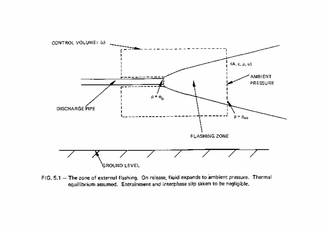
External Flashing
Consider a pressurised release of an evaporating liquid (say HF). Such a release forms at the
orifice a narrow zone in which take place pressure relaxation and violent 'flashing'. 'Flashing'
is the sudden and disruptive evaporation of superheated liquid in response to a sharp fall in
fluid pressure. This results in prompt atomisation of any residual liquid and in the
development of a two-phase flow. This stage of plume development is extremely complex.
Fortunately details of 'flashing' flow are not needed: it is sufficient to 'bridge' this zone by
means of integral conservation laws and by assuming that air entrainment during flashing is
negligible (Wheatley 1987a, Raj and Morris 1987). The flashing zone ends when approximate
thermal equilibrium, ambient pressure, and negligible inter-phase slip between vapour and
liquid (droplet) phases are established. The velocity profile is roughly uniform; the cross-
section may be assumed circular; deflection due to ambient pressure in cross-flow is typically
negligible (Figure 5.1).
Flow Establishment
Immediately beyond the flashing zone there exists a second zone 'of flow establishment': air
entrainment as the result of shear-induced turbulence results in the progressive dilution of the
evaporating liquid jet, and in the radial diffusion of air towards the plume centre-line.
The flow is described by an unperturbed 'core' region, which diffusion of air has not reached,
and by an axi-symmetric 'outer' region, in which turbulent diffusion has resulted in a near
Gaussian distribution of entrained air. This zone ends with the complete 'erosion' of the core

HGSYSTEM Technical Reference Manual
5-24
region and with the establishment of approximately self-similar conditions within the flow.
The cross-section may be assumed circular (Figure 5.2).
Generally this region is either neglected (Raj and Morris 1987; Hoot, Meroney and Peterka
1973; Forney and Droescher 1985), or else considered in conjunction with such effects as
stack 'downwash' (Hanna 1982; Ooms 1972; Havens 1987) and represented by an empirically
derived correlation (Keffer and Baines 1963, Kanatani and Greber 1972). The discussion
follows an analysis of Albertson Dai, Jensen and Hunter Rouse (1948), and of Abramovich
(1963).
Airborne Plume
Following flow establishment, plume development is described by the interaction of plume,
ambient wind, and buoyancy effects: the influence of the ground, except as a generator of
ambient turbulence and of wind-shear is negligible.
This is the simplest of all the stages of plume development: nonetheless it is not without
controversy. Arguments exists over the level of description necessary: whether Gaussian
(Ooms 1972; Ooms and Duijm 1983; Petersen 1986; Schatzmann 1979) or 'top-hat' (Hoot,
Meroney and Peterka 1973; Forney and Droescher 1985; Davidson 1986) models are
preferable; whether the effects of gradients within the atmosphere need be considered
(Schatzmann and Policastro 1984); and whether or not significant 'drag' forces act upon a
plume in cross-wind (Briggs 1984; Ooms 1972; Schatzmann 1979, Hoult, Fay and Forney
1969; Coelho and Hunt 1989).
Several different formulations for the crosswind entrainment have been proposed and checked
against experimental data (Peterson 1978, 1987; Schatzmann 1978, Spillane 1983).
Even the basic formulation of the equations of motion has resulted in discussion (Schatzmann
1978, 1979; McFarlane 1988), and in the use of special devices, such as plume 'truncation' and
dilute gas thermodynamics (Ooms 1972, Petersen 1978).
The cross-section is generally assumed to be circular; the flow axi-symmetric. However the
presence of trailing vortices in cross-flow, and the cumulative effect of differences in vertical
and horizontal diffusivity in the undisturbed atmosphere, will result in asymmetry and
ultimately in an elliptic cross-section (Bloom 1980; Li, Leijdens and Ooms 1986). The role of
dilute plume asymptotics in allowing estimation of certain entrainment coefficients from
plume-rise and other data should be emphasised. Such early work as that of Briggs (1975) in

HGSYSTEM Technical Reference Manual
5-25
the development of semi-empirical plume-rise correlations based on such analyses should not
be neglected. (Figure 5.3).
Touchdown Plume
Dense plumes must ultimately drift to ground or at any rate expand as the result of
entrainment so as to intersect the ground surface.
The ground interacts with a descending plume in several ways. First it acts as a geometrical
constraint resulting in the redistribution of plume material. Second the ground allows the
development of pressure forces as the result of pre-existing vertical momentum within the
plume. These are impact forces resulting in the conversion of vertical to horizontal
momentum. Third the ground permits the development of internal pressure within the plume
as the result of gravity-slumping, in which the transverse motion of a gravity current is driven
by an internally generated pressure acting at the ground surface. Finally drag forces must act at
the ground as the result of differences in horizontal speed between plume and ambient wind.
In this region a transition must be made between a circular cross-section appropriate to an
airborne plume, and a semi-elliptical (say) cross-section appropriate to an advected heavy-gas
plume resting upon the ground (Figure 5.4). The touchdown region is described by a cross-
section in the form of a circular segment. The region ends when a semi-circular cross-section
first develops.
This transition region is neglected by Havens (1987, 1988a) following Ooms (1972) and
Ooms and Duijm (1984), as well as (inter alia) by Bloom (1980), by Schatzmann (1979) and
by Raj and Morris (1987).
No previous model exists which attempts to make a smooth transition from airborne dense to
advected slumped plume. Limited experimental evidence does exist in the form of an
unpublished study of dense salt water plumes (Karman 1986). In addition photographic
evidence collected but not published by Hoot, Meroney and Peterka (1973) may form a useful
data set for model validation.
Slumped Plume
Following touchdown the plume cross-section may be assumed semi-elliptic. Changes in
plume eccentricity (aspect ratio) accommodate gravity slumping and the influence of residual
ground-drag and impact pressure-forces. Vertical motions will be small compared to
horizontal (Figure 5.5). An asymptotic approach, based on assumed horizontal flow,
prescribed air entrainment, and a representation of gravity-spreading, is therefore possible.

HGSYSTEM Technical Reference Manual
5-26
Such a model is that proposed by Raj and Morris (1988) for dense plumes released
horizontally at or near ground-level. The model incorporates jet entrainment, ground drag, and
a formula for dense-gas gravity spreading. This model is (however) not valid for buoyant
slumped plumes; neither is an interface for initially vertical releases provided.
Havens (1988) does not attempt to deal rigorously with the transition zone, for which
horizontal momentum may be significant, but rather makes a simple transition from first
plume/ground contact to heavy-gas advection. It may be questioned whether such a transition
is physically appropriate.
The Far-Field
Ultimately differences in velocity between (heavy-gas) plume and ambient atmosphere must
become negligible, so that the representation of the HGSYSTEM plume models or that of Raj
and Morris (1988) must merge into a heavy gas dispersion model such as HEGADAS. This is
accomplished (Chapter 7.A, section 7.A.4.2.) by means of asymptotic matching.
Alternatively for asymptotically buoyant plumes a transition may be made directly to a passive
advection (Gaussian) model such as PGPLUME (Chapter 6, Hanna 1982). It is also possible
to incorporate the observed horizontal and vertical diffusion for a passive plume into the near-
field formalism (Bloom 1980, Disselhorst 1984). This procedure is computationally costly; its
advantage over simple matching unclear.
Curiously for horizontal slumped releases Raj and Morris (1988) are content to use their
grounded jet model throughout the heavy-gas advection region, matching ultimately with a
passive advection model (Figures 5.6, 5.7). This procedure fails to make use of well-validated
models for heavy-gas dispersion.
To summarise: a review of the literature revealed clear gaps in existing models of early plume
dispersion. These relate particularly to complex thermodynamics, to plume touchdown, and to
the dispersion on the ground of possibly buoyant possibly dense clouds, such as arise for
example from the interaction of HF and moist air. There was need of a consistent
fundamentally-based model capable of describing all of the stages of plume development. No
such formalism existed prior to the development of HFPLUME. It is to the development and
validation of such a comprehensive model that this Chapter is addressed.
5.B.10. Control Volume Analysis: Basic equations of Motion
Consider a steady plume or jet issuing from a pipe break at pressure and at an angle to the
horizontal. The atmosphere into which a release takes place is in a state of steady turbulent

HGSYSTEM Technical Reference Manual
5-27
flow and has a mean wind-speed which is both horizontal and aligned with the horizontal
component of the released jet. This last assumption is inessential, and is introduced to
simplify the equations of plume motion.
We shall regard the jet and ambient atmosphere as a single fluid (of variable composition due
to entrainment of ambient air) occupying the upper half-plane above a horizontal ground-
surface. The jet and ambient atmosphere merge infinitesimally so that no jet 'boundary' exists
at finite distance from the jet-axis; entrainment occurs therefore 'at infinity'. No slip occurs
amongst the constituent phases of the developing jet; mean-flow within both ambient
atmosphere and jet/plume is everywhere steady.
We begin by introducing a set of control-volumes τ(s), s > 0, an analysis of which results in an
integral-averaged description of jet development independent of detailed assumptions
regarding induced and ambient turbulence.
The Control-Volume τ(s): First construct a vertical surface at such distance upwind of the
release-point that ambient flow is negligibly perturbed. Second, at arbitrary distance s > 0
downwind of the release-point, construct a 'cross-section' A(s) through the developing jet.
Third link these (semi-infinite) surfaces by skirting the ground and pipe-work surfaces and
passing through the jet at the plane of release. Finally construct a fourth bounding surface
A∞ at great (notionally infinite) distance from the jet-axis such as to enclose the (infinite)
volume τ(s). [See Figure 5.1-5.3; Figure 5.8]
By a 'cross-section' A(s) we intend a curved surface locally perpendicular to the (turbulent
mean) flow-velocity u. We shall assume that these surfaces form a family parameterized by a
distance s > 0 measured along a (mean flow) stream-line (the plume-axis) originating at the
point of release. Such a cross-section is orthogonal to the plume centre-line and asymptotically
vertical at great off-axis distance. It reflects the progressive rotation of the mean plume
velocity from centre-line to undisturbed atmospheric values.
We shall assume that the characteristic length-scales for plume development parallel and
perpendicular to the mean-flow are asymptotically ordered, at any rate in those regions of the
flow for which departures between the plume and undisturbed ambient flows are significant.
Specifically we shall take the parallel length-scale to be much greater than the perpendicular:
it is in this sense that the jet/plume may be described, following Hinze (1959), as 'thin'. Finally
we shall have regard to that part of the ground surface over which there exist significant
departures from the undisturbed ambient either in pollutant concentration, in pressure, or in
ground-shear. This area, the intersection of plume and ground, we term the plume 'footprint'
F(s).

HGSYSTEM Technical Reference Manual
5-28
Integration of the basic equations of motion over such a control-volume results, given an
assumed 'thin' jet, in the integral forms (Hinze 1959):
Pollutant mass-flux
c d c dm dtA s
u A⋅ =zz( )
( / ) /0 0 0ρ (34)
Entrained mass-flux
( ) ( )( ) ( )
ρ ρ ρ ρ ρu u A A u u u A− ⋅ = ⋅ − − ⋅∞ ∞ ∞ ∞zz zz∞
d dA S A s
0 0 0 (35)
Horizontal excess-momentum flux
ρ φu e A( ) ( ) ( ) / cos ( )( )
,u u p p d u u dm dt A p px x
A s
x− + − ⋅ = − + − +∞ ∞ ∞ ∞zz 0 0 0 0 0
(36)
− ⋅∇ − −∞∞zzzzzρ τ
τ
u u d dAxz xz
F ss
( )( )( )
Σ Σ
Vertical momentum flux
[ ( ) ] / sin ( ),
( )
ρ φu e Au p p d u dm dt A p pz z z
A s
+ − ⋅ = + −∞ ∞zz 0 0 0 0 0
(37)
− − + −∞ ∞zzzzz ( ) ( )( )( )
ρ ρ ττ
g d p p dAF ss
Total energy flux
[ ( )] ( )( ) ( )
ρu u u Ah h d dAA s
a
F s
+ − − ⋅ = − +∞ ∞zz zz12
2 12
2 Φ Φ
(38)
+ + − − − ⋅∇ + +∞ ∞ ∞ ∞zzz( ) / ( ), ,
( )
h u h u dm dt h u gz ds
01
2 02
01
2 02
012
2ρ ττ
u
Notation: vectors are given in bold type and the '⋅' denotes a vector product, dm/dt0, mass
flow-rate issuing from the release-point; (ρ,c,u,p,h), density, pollutant mass-concentration,
velocity, absolute pressure, and specific enthalpy of the ensemble-averaged flow. φ angle to

HGSYSTEM Technical Reference Manual
5-29
the horizontal of the plume-axis (co-ordinate stream-line), Φ the surface to air heat-flux, åxz
the Reynolds stress as the result (ultimately) of viscous drag at the ground. ex and ey denote
unit vectors in the horizontal (wind aligned) and vertical (upward) directions. The affix '0'
identifies conditions at the release-plane; the suffix '¥' conditions within the unperturbed
atmosphere.
These equations express in integral form conservation of pollutant (e.g. HF) mass-flux, air
entrainment, conservation of the excess above ambient of momentum (both horizontal and
vertical), and conservation of energy.
The pollutant continuity equation (Pollutant mass-flux) expresses that the released pollutant
(for example HF), is merely transported and diluted by the atmosphere.
Total mass continuity (Entrained mass-flux) allows the identification of the entrained air
mass-flux with the integrated sum of mass-flows induced 'at infinity', that is at great distance
from the plume centre-line. The equation is formulated as a difference in mass-flux between
the undisturbed atmosphere and the system that exists following a sustained release of a
pollutant. This has advantages over conventional (total mass-flux) formulations (Ooms 1972,
Petersen 1987) in that it is not necessary to introduce a 'cut-off' point in a Gaussian plume
model beyond which conditions revert (discontinuously) to atmosphere values (Schatzmann
1978). This permits true Gaussian profiles to be introduced in estimating concentrations and
temperatures within the developing plume or jet, with a consequent improvement in the
accuracy of predicted centre-line concentrations (Davidson 1986, McFarlane 1988).
The horizontal momentum equation (Horizontal excess-momentum flux) states that (in the
absence of ground drag and significant vertical wind-shear) the excess-flux of horizontal
momentum is conserved. Horizontal momentum excess is therefore a natural variable of the
jet/plume system (Hinze 1959, McFarlane 1988). Conventional plume models neglect
'ground-effects' (have zero 'footprint' area) and consider only the weak effect of vertical wind-
shear upon horizontal momentum flux. The present model, in dealing consistently with 'jet',
buoyant plume, and 'slumped' plume, necessarily incorporates a ground-drag force, acting over
the plume 'footprint', the effect of which is (substantially) to decelerate an 'airborne' plume at
first ground 'impact'. Note that the drag force is expressed over the 'footprint' area F(s), and in
terms of the difference between the ground-level stresses Σxz and Σxz∞ in the presence or
absence of released material. Clearly drag forces exist even in the undisturbed atmosphere:
these, however, are balanced in steady atmosphere flow by (weak) horizontal gradients in the
ambient pressure field, and are therefore absent from the difference formulation adopted here.

HGSYSTEM Technical Reference Manual
5-30
The vertical momentum equation (Vertical momentum-flux) expresses the variation in the
flux of vertical momentum in terms of forces arising from either buoyancy or pressures
developed at the ground surface at 'touchdown' and beyond. Conventional descriptions model
either buoyancy forces alone, or else buoyancy together with 'airborne' plume drag, that is the
pressure force that arises over the cross-section A(s) as the result of small local differences
between undisturbed ambient and plume pressure (Frick 1984).
'Airborne' drag is a controversial element (Briggs 1984), being found necessary by some
(Ooms 1972, Petersen 1978, Schatzmann 1979) but not by others (Petersen 1987; Forney and
Droescher 1985; Hoot, Meroney and Peterka 1973). The present model necessarily includes
pressure forces developed over the plume 'footprint' in response to velocity changes implied
by air entrainment, buoyancy, ground-drag, and the geometrical constraint of an impermeable
(level) ground. Pressure forces at the ground develop in response to the interaction of 'top'
entrainment and 'gravity slumping', and hence are plausibly expressed in terms of the
spreading velocity and buoyancy force in a manner consistent with the gravity current
spreading (van Ulden 1984, Raj and Morris 1987).
Finally consider the energy equation (Total energy flux), which expresses the near constancy
of the excess flux above ambient values of the plume total energy (essentially enthalpy). This
flux is altered by small vertical gradients in atmospheric enthalpy and wind-speed, and by the
potential energy changes associated with vertical motion under terrestrial gravity The
'airborne' plume is assumed to exert negligible influence on the heat transfer from ground to
atmosphere. In addition for a touchdown plume whose temperature differs substantially from
that of the ground the heat flux at the ground surface may become important. The heat-flux
from the ground is mediated via a heat transfer coefficient the magnitude of which is related to
the vertical turbulent transport of heat from ground surface into the overlying plume. For the
unperturbed atmosphere such fluxes are also present but are balanced by vertical temperature
gradients and by (typically small) systematic variation in temperature downwind. This
unperturbed heat flux is therefore absent from the difference model here developed, except
inasmuch as it determines the Monin-Obukhov length, wind-speed and temperature profiles
within the undisturbed atmosphere (Plate 1982, Colenbrander 1985). No provision has been
made for this enhanced ground/plume heat transfer in the current model formulation. Such
provision is however encoded within the heavy-gas advection module HEGADAS.
Inasmuch as the HGSYSTEM plume models are intended as a 'front-end' to a heavy-gas
advection model such as HEGADAS, the neglect of heat transfer from the ground at
touchdown and beyond was judged insignificant.

HGSYSTEM Technical Reference Manual
5-31
5.B.11. External flashing; Flow Establishment; Gaussian profiles
This section 'bridges' the external flash (depressurisation) and flow-establishment zones prior
to the development within a released plume/jet of (approximately) self-similar conditions. The
discussion of flow establishment relates particularly to the prediction of point-local from
sectionally averaged concentrations within the early jet, and to the prediction of the zone
length. This analysis is not incorporated within the (integral averaged) HGSYSTEM plume
models. Such detailed formulation (as it affects air entrainment) requires careful experimental
validation and exerts a modest influence upon predictions in the range of greatest interest,
perhaps 10 to 500 m downwind of release; it has, however, clear implications for a purely
Gaussian plume model.
External Flashing
Having set up the basic equations of motion in integral form, we specialise in order to 'bridge'
the external flashing zone, or for a gas-jet the depressurisation zone, that occurs immediately
beyond the breakpoint in choked flow. In the absence of choked flow this transitional region
may still be present. For example, for a purely liquid release, pressure at the orifice may be an
appreciable fraction of the storage (reservoir) pressure; this pressure, however, rapidly relaxes
within the vena contracta to an essentially ambient value. During flashing radial and axial
velocities within the developing jet are of co-magnitude so that the 'thin jet' approximation is
invalid. In addition interphase slip and thermal disequilibrium are likely to occur.
Nonetheless depressurisation occurs so quickly, within a few (perhaps 5) diameters of the
release plane, that 'thin jet', equilibrated conditions may be presumed to exist everywhere
except within a narrow transition zone adjacent to the release point. We shall assume further,
in view of the strongly expanding flow of a flashing jet, or the very large density differences
between jet and ambient of a liquid jet, that negligible air entrainment occurs within this
depressurisation zone. The length of the zone will in the context of evaporating liquid jets or
plumes ordinarily be negligible and will hereafter be ignored: the models have initial
conditions defined 'immediately post flash' at (axial) displacement zero.
Neglecting further the influence of gravity and of wind-shear upon the integral conservation
laws, we deduce, for the conditions 'immediately post flash', the elementary forms (Figure 5.1)
u uA p p
dm dt= +
− ∞0
0 0
0
( )
/
c = ρ
φ φ= 0 (39)

HGSYSTEM Technical Reference Manual
5-32
A c u dm dt= / 0
h u h u h u h u+ − − = + − −∞ ∞ ∞ ∞12
2 0 12 0
20
12 0
2 0 12 0
2, ,
The notation is that φ is the angle of inclination to the horizontal, and that A0 is the (true) area
of the release orifice. The values of velocity u, density ρ, and area A are averaged values, that
is they assume an essentially uniform velocity or density within the jet as it emerges from the
depressurisation zone.
This is approximately valid for a liquid jet, (Albertson, Dai, Jensen, and Hunter Rouse 1948)
and is at any rate plausible for a gaseous or two-phase jet. Certainly drag forces at the jet edge
and the momentum redistribution associated with the entrainment of air are for consistency
necessarily small.
Flow Establishment
Beyond the zone of depressurisation there exists a second transitional zone, a zone of 'flow
establishment', in which the interaction of jet and ambient result in the progressive turbulent
diffusion of air towards, and of jet momentum away from, the jet centre-line. This zone is
characterised by a progressive change from a 'top-hat' velocity profile to an essentially
Gaussian profile (Hinze 1959, Abramovich 1963) in the asymptotic far-field. Within this
zone, neither 'top-hat' nor Gaussian profiles properly describe the cross-sectional variation in
jet velocity and pollutant concentration (Figure 5.2).
What is needed is a transitional profile (Albertson, Dai, Jensen, and Hunter Rouse 1948) in
which an inner 'core' jet (of uniform velocity and pollutant concentration of 100 %) is 'eroded'
by a spreading Gaussian profile coupling inner 'core' and outer ambient flows. An order of
magnitude analysis yield that this zone is of typical length l/D= 1/ejet, in which D is a
representative diameter 'immediately post flash', and in which ejet is a (dimensionless)
coefficient whose magnitude measures the effectiveness of jet/ambient shear in causing air
entrainment.
For gas jets this magnitude is most probably comparable to that seen following the
establishment of self-similar flow (Ricou and Spalding 1961), which for a 'top-hat' model
yields a value ejet = 0.08. This is certainly reduced for a two-phase system (McFarlane 1988),
and may be much smaller for a liquid jet for which dynamical break-up, rather than flashing
'atomisation', may dictate the entrainment rate (Wheatley 1987a, Ohnesorge 1936, van de
Sande and Smith 1976, McCarthy and Molloy 1973).
HGSYSTEM Technical Reference Manual
5-33
We shall assume that all modelled releases result in prompt atomisation rather than gradual
break-up, as is consistent with the earlier assumptions of negligible interphase slip and
thermodynamic equilibrium. This results in a zone of flow establishment whose length is
perhaps 20 orifice diameters. This zone is therefore also of a negligible length compared with
downwind displacements of orders ten or hundred metres.
More complex models are possible and have been suggested (Jones 1988, Ianello and Rothe
1988): they require further and uncertain details regarding jet and droplet break-up and
evaporation.
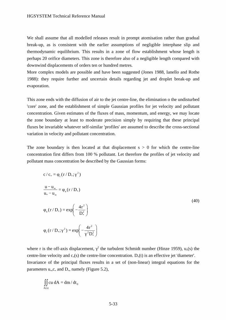
This zone ends with the diffusion of air to the jet centre-line, the elimination o the undisturbed
'core' zone, and the establishment of simple Gaussian profiles for jet velocity and pollutant
concentration. Given estimates of the fluxes of mass, momentum, and energy, we may locate
the zone boundary at least to moderate precision simply by requiring that these principal
fluxes be invariable whatever self-similar 'profiles' are assumed to describe the cross-sectional
variation in velocity and pollutant concentration.
The zone boundary is then located at that displacement s > 0 for which the centre-line
concentration first differs from 100 % pollutant. Let therefore the profiles of jet velocity and
pollutant mass concentration be described by the Gaussian forms:
c c r Dc/ ( / ; )* *= φ γ 2
u u
u ur Du
−−
=∞
∞**( / )φ
(40)
φu r Dr
D( / ) exp*
*
= −FHG
IKJ
4 2
2
φ γγc r D
r
D( / ; ) exp*
*
22
2 2
4= −
FHG
IKJ
where r is the off-axis displacement, γ2 the turbulent Schmidt number (Hinze 1959), u*(s) the
centre-line velocity and c*(s) the centre-line concentration. D*(t) is an effective jet 'diameter'.
Invariance of the principal fluxes results in a set of (non-linear) integral equations for the
parameters u*,c* and D*, namely (Figure 5.2),
cu dA dm dtA s( )
/zz = 0

HGSYSTEM Technical Reference Manual
5-34
( ) /( )
ρ ρu u dA dm dtA s
− =∞ ∞zzρu u u dA dP dt u dm dt
A s
x( ) / /( )
− = −∞ ∞zzwhere dm/dt0 is the pollutant mass flux coming from the orifice and dm/dt is the total plume
mass flux at any location (pollutant plus entrained air).
The above non-linear system has a solution space which properly contains the set of physically
admissible 'self-similar' profiles. Additionally a-physical solutions exist for which c* > ρ*, that
is for which the pollutant mass-concentration exceeds the total mixture density; for which u* >
upost flash, that is for which the centre-line velocity is greater than the velocity immediately post
flash; and finally for which c* > cpost flash, that is for which the centre-line concentration,
consistent with an assumed Gaussian profile, actually exceeds that found at the jet-axis
immediately following jet depressurisation.
The correct diagnosis from these symptoms is that the set of principal fluxes (dm/dt0 , dm/dt,
dPx/dt) and the atmosphere properties (ρ∞, u∞) correspond not to Gaussian self-similarity, but
rather to a cross-section located within the zone of flow development. The zone boundary is
therefore defined by the simultaneous solution of the above integral equations, together with
the 'boundary equation', c* = cpost flash
5.B.12. The Airborne Plume: geometry and shear entrainment
We consider in this section the representation of the 'airborne' plume, that is the plume from a
point 'immediately post flashing' to the point of first plume 'touchdown'. We have chosen to
represent the plume development in terms of a simple, integral-averaged, or 'top-hat' model in
which is tracked the plume 'centre-line'. The plume consists of a set of circular cross-sections,
each of defined diameter, mean density, temperature, and mass concentration of pollutant.
Within each cross-section the velocity is assumed uniform; outside conditions are those of the
undisturbed atmosphere.
We seek to introduce a (global) co-ordinate system the level surfaces of which are everywhere
orthogonal to the turbulent-mean flow. Such co-ordinates, however, cannot be found without
detailed knowledge of the turbulent flow in the presence of a dense-gas plume. In the
circumstances we must be content with an approximate co-ordinate description valid in the
neighbourhood of the plume-axis. We begin by introducing a local ('canonical') co-ordinate

HGSYSTEM Technical Reference Manual
5-35
system (s,r,θ) defined in the neighbourhood of the plume centre-line (Figures 5.8, 5.9,
Schatzmann 1978):
r x y z r ds ds rs s
= = + + −z z( , , ) ( cos , , sin ) ( sin sin ,cos ,cos sin )0
0 0
0φ φ φ θ θ φ θ (41)
with r x y z s r s r0 0 0 0 0 02
3
20 2= ≤ ≤ ∞ ≤ ≤ ∞ − ≤ ≤ ≤ ≤( , , ); ( , , ): , , ,θ
πφ
πθ π
The co-ordinate s marks the distance along the plume centre-line from release point to a
general plume cross-section A(s). The co-ordinate pair (r,θ) defines a set of plane polar co-
ordinates in the cross-section A(s). The angle φ(s) is the inclination of the plume centre-line at
displacement s from the release point (Figure 5.3).
Such co-ordinates are not and cannot be globally defined. Neither do the level surfaces ds = 0
coincide precisely with the surface A(s) in the sense of the original control-volumes t(s) of
section 5.B.3. In particular the level surface ds = 0 are not asymptotically vertical as are the
original surfaces A(s). They do nonetheless approximate such cross-sections A(s) in the
vicinity of the plume centre-line, that is in that region of the plume for which the differences
between plume and ambient are most pronounced. This certainly suggests, though it cannot
confirm that it is legitimate to cast the equations of plume motion in terms of a 'top-hat' model
and its associated, 'canonical', co-ordinate system.
Differentiation of the integral equations of section 5.B.3. then yields, for the canonical co-
ordinates (s,r,θ), the basic differential equations;
d/ds(dm/dt) = EntrAmbA(s) ;
d/ds(dPx/dt) = -DragAmbA(s) .ex - ShearAmb
A(s)
d/ds(dPz/dt) = -DragAmbA(s) .ez - BuoyAmb
A(s) ;
(42)
d/ds(dE/dt) = -EnerAmbA(s)
dx/ds = cosφ
dz/ds = sinφ
together with the algebraic constraints

HGSYSTEM Technical Reference Manual
5-36
A = (p/4) D2
dm/dt = A ρ u
dm/dt0 = A c u
(43)
dPz/dt = dm/dt u sinφ
dPx/dt =dm/dt (u cosφ - u¥)
dE/dt = dm/dt (h + ½u2 - h¥ - ½u¥2)
Notation: A cross-section area, D plume diameter (circle), x horizontal axis-displacement, z
axis height above level ground, dm/dt released and entrained mass-flux, (dPx/dt, dPz/dt) excess
(horizontal, vertical) momentum flux, dE/dt excess energy flux, dm/dt0 pollutant mass-flux; u
mean flow-speed, φ axis inclination, ρ mean plume-density, c mean pollutant mass-
concentration, h(ρ,c,P¥) specific enthalpy the suffix '¥' denotes ambient conditions at the
centroid height z > 0.
The quantities Drag, Shear, Entr, Buoy, and Ener have the formal definitions,
DragAmbA(s) = (d/ds)
A s( )zz (p - p¥)dA (44)
ShearAmbA(s) =
A s( )zz ρ sinφ (du¥/dz) ½J½/r dA (45)
EntrAmbA(s) =
A∞
zz ρ u.dA (46)
BuoyAmbA(s) =
A s( )zz (ρ - ρ¥) g½J½/r dA (47)
EnerAmbA(s) =
A s( )zz ρ u sinφ (d/dz) (h¥ + ½u∞
2 + gz) ½J½/r dA (48)
Notation: s displacement along plume centre-line, z height above ground, f plume centre-line
inclination, ρ local (turbulent averaged) density, u flow-speed, p (absolute) pressure, h specific
enthalpy, ½J½= r-r2 sinθ df /ds Jacobian determinant, g acceleration due to gravity, dA = rdrd
θ (scalar) area element.

HGSYSTEM Technical Reference Manual
5-37
They represent (respectively) the 'drag' force DragAmbA(s) acting on the plume in cross-flow as the
result of vortex formation in the plume wake (Ooms 1972, Schatzmann 1979), the shear force
ShearAmbA(s) associated with the vertical gradient of wind-speed, the total entrainment rate
EntrAmbA(s) per unit axis length, the section-averaged buoyancy force BuoyAmb
A(s) , and the variation
in plume total energy EnerAmbA(s) resulting from vertical gradients of temperature (enthalpy) and
wind-speed.
The pressure is that deduced for hydrostatic equilibrium, except insofar as departures result in
the (airborne) drag force.
These integrals are in actual practice replaced by empirical formulae chosen for compatibility
with existing plume models and literature available data. These formulae express, for
example, the contribution to air entrainment within the plume of the difference in velocity
between mean cross-sectional velocity and the ambient wind-speed. Model closure is
therefore in terms solely of mean cross-sectional and local atmospheric ambient parameters.
The above 'algebraic constraints' can be viewed as definitions of, for example, the total mass-
flux within the plume, or the area of a circle. It is algebraically convenient to regard these as
algebraic equations forming part of a differential/algebraic system. Such a system is then
solved by means of the differential/algebraic package SPRINT (Berzins, Dew, and Furzeland
1983; Berzins and Furzeland 1985). Such a formulation allows the somewhat different
descriptions of 'touchdown' and 'slumped' plumes to be incorporated within the same
formalism.
5.B.13. The Touchdown and Slumped Plume
Consider next the representation of the plume following first 'touchdown'. Touchdown occurs
at that axial displacement s > 0 for which an assumed circular cross-section just touches the
horizontal ground surface z = 0.
It is also the point beyond which the plume footprint width first assumes a non-zero value.
The cross-section of a plume following touchdown is modelled not by a circle but rather by a
circular segment. This centroid location will, for a dense plume, continue to fall, so that after
some time a semicircular cross section is certain to arise. At this point the plume has passed
through a transitional region between circular 'airborne' and semi-elliptic 'slumped' cross-
sections. Further development will, at least initially, be characterised by (transverse) gravity
spreading (van Ulden 1974, Raj and Morris 1987), and by air entrainment principally through
the 'upper' plume surface.

HGSYSTEM Technical Reference Manual
5-38
These elements may be assembled within the framework of a 'top-hat' model as the differential
system:
d/ds(dm/dt) = EntrAmbA(s)
d/ds(dPx/dt) = -DragAmbA(s) .ex - ShearAmb
A(s)
d/ds(dPz/dt) = -DragAmbA(s) .ez - BuoyAmb
A(s) + FootAmbF(s)
(49)
d/ds(dE/dt) = EnerAmbA(s)
dx/ds = cosφ
dz/ds = sinφ
together with the algebraic constraints
'Touchdown' Plume
AD
c c= − + −−2
1 2
41cos ( )η η
dm/dt = A ρ u
dm/dt0 = A c u
dPz/dt = dm/dt u sinφ
dPx/dt = dm/dt (u cosφ - u¥) (50)
dE/dt = dm/dt (h + ½u2 - h¥ - ½u¥2)
η ηη
η η ηc
c
c c c
= −−
− + −
RS|T|
UV|W|−
2
3
1
1
32
1 2
b gcos ( )
ηφ
=2z
D cos
ηφc
cz
D=
2
cos
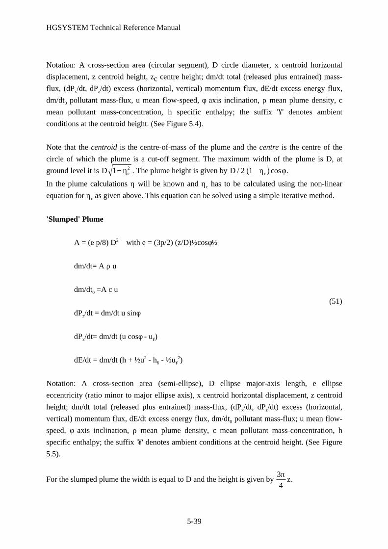
HGSYSTEM Technical Reference Manual
5-39
Notation: A cross-section area (circular segment), D circle diameter, x centroid horizontal
displacement, z centroid height, zc centre height; dm/dt total (released plus entrained) mass-
flux, (dPx/dt, dPz/dt) excess (horizontal, vertical) momentum flux, dE/dt excess energy flux,
dm/dt0 pollutant mass-flux, u mean flow-speed, φ axis inclination, ρ mean plume density, c
mean pollutant mass-concentration, h specific enthalpy; the suffix '¥' denotes ambient
conditions at the centroid height. (See Figure 5.4).
Note that the centroid is the centre-of-mass of the plume and the centre is the centre of the
circle of which the plume is a cut-off segment. The maximum width of the plume is D, at
ground level it is D c1 2− η . The plume height is given by D c/ ( ) cos2 1+ η φ .
In the plume calculations η will be known and ηc has to be calculated using the non-linear
equation for ηc as given above. This equation can be solved using a simple iterative method.
'Slumped' Plume
A = (e p/8) D2 with e = (3p/2) (z/D)½cosφ½
dm/dt= A ρ u
dm/dt0 =A c u
(51)
dPz/dt = dm/dt u sinφ
dPx/dt= dm/dt (u cosφ - u¥)
dE/dt = dm/dt (h + ½u2 - h¥ - ½u¥2)
Notation: A cross-section area (semi-ellipse), D ellipse major-axis length, e ellipse
eccentricity (ratio minor to major ellipse axis), x centroid horizontal displacement, z centroid
height; dm/dt total (released plus entrained) mass-flux, (dPx/dt, dPz/dt) excess (horizontal,
vertical) momentum flux, dE/dt excess energy flux, dm/dt0 pollutant mass-flux; u mean flow-
speed, φ axis inclination, ρ mean plume density, c mean pollutant mass-concentration, h
specific enthalpy; the suffix '¥' denotes ambient conditions at the centroid height. (See Figure
5.5).
For the slumped plume the width is equal to D and the height is given by 3
4
πz.

HGSYSTEM Technical Reference Manual
5-40
Note that the differential system is modified in that, in addition to any 'airborne' drag forces,
we have (generally significant) 'ground' drag associated with the strong shear layer at the
ground-surface following plume touchdown. A further (pressure) force FootAmbF(s) is exerted at
the ground surface as the result either of the destruction of vertical momentum impacting the
ground, or in response to a pressure build-up associated with the limited (gravity-slumping)
rate of transverse plume expansion. These additional forces exist following touchdown and in
the slumped plume regime. They have the formal definitions:
FootAmbF(s) = (d/ds)
F s( )zz (p - p¥)dA (52)
DragAmbF(s) = (d/ds)
F s( )zz (åxz - åxz
∞ )dA (53)
and are replaced in the actual plume models by intuitively derived functions which reflect
known spreading and impact behaviour.
For the circular cut-off segment the cross-sectional area A and centroid height z are not
explicitly related but coupled via a single non-linear equation for the geometric centre zc. In
the case of the slumped plume both the area A and centroid height z are related to the
eccentricity e of the semi-ellipse; however the eccentricity is given explicitly in terms of
known parameters z, φ, and D.
5.B.14. Closure Assumptions for the 'Top-Hat' Model
In this section are considered the assumptions, arguments, and simplifications that enable
closure of the 'top-hat' model: We shall ask: 'Which expressions and what coefficient values
are appropriate for the formulation of impact forces, drag forces, and buoyancy in each of the
three plume regions; airborne, touchdown, and slumped plume?'.
Atmosphere-Gradient Induced Forces: Plume Buoyancy:We begin by considering the simplest of these functions, ShearAmb
A(s) , EnerAmbA(s) , and BuoyAmb
A(s) , and
take first of all the buoyancy force BuoyAmbA(s) . This has the formal definition,
BuoyAmbA(s) =
A s( )zz (ρ - ρ¥) g ½J½/r dA (54)
in which the Jacobian determinant has the value
½J½= r - r2 sinθ dφ/ds, ½J½ > 0 (55)

HGSYSTEM Technical Reference Manual
5-41
The buoyancy term is well approximated by the simple expression,
BuoyAmbA(s) = A (ρ - ρ¥) g (56)
a result which extends for expansion about the plume centroid (centre-of-mass) for both
touchdown and slumped plume.
Analyses and order of magnitude arguments yield analogous results for the functions
ShearAmbA(s) , and EnerAmb
A(s) . It follows that
ShearAmbA(s) = dm/dt sinφ du¥/dz (57)
EnerAmbA(s) = dm/dt sinφ (d/dz)[h¥ + ½u¥
2 + gz] (58)
Airborne Drag
Consider next the 'drag' function associated with an airborne plume in cross-flow. This
function represents the force acting upon the plume as the result of pressure forces created by
trailing (wake) vortices. The term 'drag' is by analogy to the drag force exerted upon a rigid
body immersed in a uniform stream.
There are, however, major differences between the pressure field of a fluid jet and of a
(geometrically similar) rigid body. Firstly there is no sharply defined boundary at which the
'no slip' condition may be applied. Secondly the external flow, and hence the boundary
integral of pressure, may differ substantially between plume and body.
The analogy is therefore weak, so that not only the coefficient magnitudes but also the
functional form appropriate to a rigid body may be questioned when applied to a plume in
cross-flow. The form and magnitude of this airborne drag force is therefore particularly
uncertain. It is found necessary by some (Ooms 1972, Petersen 1978, Schatzmann 1978), but
not by others (Hoot, Meroney and Peterka 1973; Hoult, Fay and Forney 1969; Petersen 1987).
A recent study (Coelho and Hunt 1989) of the near-field following release orthogonal to a
steady flow found no evidence either experimental or theoretical for a significant 'drag' force.
Plume deflection was satisfactorily explained by air entrainment alone.
We assume that
DragAmbA(s) = 0 (59)
Plume impact Forces

HGSYSTEM Technical Reference Manual
5-42
Consider next the pressure forces exerted over the plume 'footprint' for a touchdown or
slumped plume. These forces arise from two distinct physical mechanisms: the destruction of
momentum associated with the impact of a dense plume upon the ground surface; and the
pressurisation associated with the gravity-limited rate of lateral plume spreading.
Take first the case of a plume impacting the ground surface (Figure 5.10). The assumption of
an elastic collision applied to the plume as a whole requires that the impact pressure force be
at right angles to the momentary orientation of the centroid axis. This ensures conservation of
kinetic energy for a system without entrainment or other disturbing influences such as gravity.
Focus next upon that proportion of the descending plume impinging upon level ground in time
dt > 0.
If the footprint is of width l then the impinging momentum flux is correspondingly,
dP = dA ρ u(cosφ, 0, sinφ); dA = l u½tanφ½dt (60)
in which dA is the sectional area 'absorbed' into the ground surface.
We assume further that the magnitude of the impact force is such as to destroy completely the
momentum-flux impinging at any instant upon the ground. The impact pressure force is
therefore,
ImpactAmbF(s) = l ρ u2½tanφ½(sinφ, 0, -cosφ); sinφ ³ 0 (61)
This formula differs somewhat from that expected from the control-volume analysis, in that
both horizontal and vertical moments undergo continuous change. The pressure force integral
implies a change solely in the vertical momentum. Additionally consideration of the
destruction of horizontal momentum yields that flows in the negative x-direction are induced
for impact angles in excess of 45°.
Certainly, for vertical incidence, the spreading pattern is axi-symmetric about the point of
impact except inasmuch as this is modified by the ambient wind. For steeply descending
plumes, therefore, upwind spreading, vortex formation, and flow separation make a simple
transition described in terms of a continuous mean-flow at least difficult. However, for
shallow incidence, such upwind spreading is typically absent, so that a 'top-hat' transition
remains entirely feasible.
The form of the impact force ImpactAmbF(s) implies a transition between 'steeply descending' and
'shallow incidence' plumes at an angle of descent φ = 45°. This is precisely the value observed
experimentally by Karman (1986). We restrict attention, therefore, to plume touchdown at
angles φ less than 45°. Steeply descending plumes will require either empirical matching of

HGSYSTEM Technical Reference Manual
5-43
airborne and slumped plumes (Karman 1986), or else matching to a 'spreading pool' model,
possibly analogous to the HGSYSTEM area source slumping model HEXABOX.
In addition, in the absence of air entrainment or drag forces, such as would describe shallow
incidence impact of a liquid jet, the above impact force implies that the mean jet/plume speed
remains constant throughout the impact process. This is consistent with a direct application of
Bernoulli's theorem, gravity and ground drag being negligible, and is consistent with the
impact of a liquid jet on a curved vane (Fox 1974). For this case the horizontal impact force
evidently arises from pressure components developed along the curved surface of the
deflecting vane. For the actual case of ground impact we may 'square the above circle' by
regarding the jet/plume as existing above a recirculating flow the common interface of which
is the analogue of the physical vane. In the immediate vicinity of first ground impact,
therefore, the top-hat model represents not the complete flow but only the non-recirculating
portion. Plume impact may then be modelled as a simple (elastic) collision.
Gravity-Slumping Pressure Forces
Consider next the pressure force induced over the plume 'footprint' by the interaction of ('top')
entrainment and gravity-'slumping'. This pressure arises from the fact that entrainment may
increase the cross-sectional mass-flux at a rate incompatible with a prescribed gravity-
spreading unless the centre of mass is also raised. Such a raising of the centre of mass against
gravity can be accomplished only by means of a pressure force acting over the plume
footprint. The absolute magnitude of this pressure is small; its integrated effect significant. Let
us begin (refer Figure 5.11) with the gravity-spreading relation (van Ulden 1983, Raj and
Morris 1987) for a rectangular, 'slumped' jet
½dD/ds = (k/u) g h(1 - / )ρ ρ∞ (62)
Notation: h plume height, D plume width, g acceleration due to gravity, (ρ,u) mean density
and flow-speed, ρ¥ ambient density, k (0.85-1.20) empirical coefficient, s centre-line
displacement.
We seek a formulation for the vertical momentum equation such that this gravity-slumping
behaviour is asymptotically recovered for dense, advected plumes. For such a plume the
spatial rate of change of vertical momentum is undoubtedly small, that is the sum of vertical
forces is approximately zero. We interpret Raj's formula for gravity spreading as a statement
of the approximate balance of a buoyancy force, and the reactive pressure force driven by the
interaction of slumping and entrainment. Given, therefore, that the buoyancy force has the
form,

HGSYSTEM Technical Reference Manual
5-44
BuoyAmbA(s) = h D g (ρ - ρ¥) (63)
we propose a reactive pressure force,
FootAmbF(s) = (1/k2) D ρ u2 [½dD/ds]2 (64)
proportional to the local footprint width, and to the square of the lateral spreading velocity.
In the case of a semi-elliptic cross-section we must reinterpret the lateral spreading velocity,
and effective plume height h in terms of the plume width D and centroid height z.
The height h is for a rectangular section exactly twice the centroid height which allows the
identification h = 2z. Additionally the rectangular section has area hD equal to that of a semi-
ellipse (3p2/16)zD of centroid z and footprint width D.
This results in the final expression, modified for the semi-elliptic geometry
FootAmbF(s) = (3p2/32)3 (1/k2) l ρ u2 [½dD/ds]2, k = 1.15 (65)
We follow van Ulden (1983), rather than Raj and Morris (1988) in the choice of the gravity-
spreading coefficient. Further work is, however, necessary in order optimally to determine the
coefficient value for a semi-elliptic, slumped plume.
This revised formulation will evidently reproduce the gravity spreading behaviour 'hard-wired'
by Raj and Morris (1988). It is, moreover, physically meaningful for an asymptotically neutral
or buoyant plume/jet for which significant departures from gravity-spreading must be
expected. In particular the original spreading formula is not defined for a buoyant plume.
Initially dense, subsequently buoyant, plumes occur frequently for the release of pressurised
liquid HF or other liquid gases, to ambient atmospheres of moderate humidity (> 50 %) and
temperature (perhaps 20 °C).
Gravity Current Collapse
Gravity spreading as formulated by van Ulden (1983) and Puttock (1988) assumes the
existence of a (relatively) sharp interface between plume and undisturbed air. Recent
experiments by Linden and Simpson (1988) indicate that the leading vortex of such a gravity
current is not unconditionally stable but may be disrupted by locally enhanced turbulence.
Following gravity current collapse the cloud edge is more diffuse; lateral spreading much
reduced.

HGSYSTEM Technical Reference Manual
5-45
Study of the HTAG ('Heavier than Air Gas') data set (Petersen and Ratcliff 1989), reveals
evidence for the existence of such gravity current collapse for uniform ambient turbulence and
increasingly weak gravity-head. We propose a collapse criterion and post-collapse spreading
rate (essentially) as follows:
½dD/ds = (2 ρ¥ u* h)/(3 k CD u D) Ri* F(Ri*) (66)
ρ ρκ∞ >/ ( )* *
D
hRi Ri
16
3Φ (67)
Φ( )
/
max( , /
*
*
*
**
Ri
RiRi
RiRi
=
−<
≤ <
+ ≥
R
S
|||
T
|||
1
1 3 50
1189
80
7
10
171 4 5
189
80
0 Ri
) Ri
*
*
(68)
with Ri* = g h (ρ - ρ∞) and h = 2z.
Notation: h plume height, D plume width, g acceleration due to gravity, (ρ,u) mean density
and flow-speed, ρ¥ ambient density, κ is the Von Kármán constant, CD (with value 5.0)
empirical (spreading) coefficient, s centre-line displacement, u* friction velocity, Ri* (bulk)
Richardson number ; F(Ri*) heavy gas entrainment function.
Spreading, 'post collapse', is represented in the HGSYSTEM plume models by the limit of the
vertical momentum equation for which the corresponding 'footprint' force is simply
FootAmbF(s) = (3p2/64)3 (3 k CD/F(Ri*)) l ρ u u* (D/z) dD/ds (69)
ρρ π
κ∞ >D
zRi Ri
1024
9 2 * *( ) /Φ (70)
with CD = 5.0 and Ri* = 2 g z (ρ/ρ¥ - 1)/u*2
The possibility exists that a gravity current may reform following initial turbulent collapse.
Intuition suggests that such reformation may occur, but that the collapsed state is 'metastable',
that is vortex (re-) formation may be considerably delayed. In the absence of detailed
experimental evidence, we may presume gravity current collapse irreversible.

HGSYSTEM Technical Reference Manual
5-46
Ground-surface Drag
Finally we consider the drag force exerted at the ground surface by an impacting or slumped
plume. This force has the formal definition
DragAmbF(s) = (d/ds)
F s( )zz (åxz - åxz
∞ ) dA (71)
and results from differences in the mean horizontal and undisturbed wind speeds in the
neighbourhood of the ground surface. The surface stress associated with the wind profile is
ρ¥u*2, in which u*
is the friction velocity.
Equivalently åxz∞ is proportional to the square of the velocity gradient du¥/dz at the roughness
height zr > 0.
Profile information regarding the vertical variation in flow-speed within the impacting or
slumped plume is therefore necessary in order to estimate the drag force. For an assumed
neutrally buoyant plume and a logarithmic velocity profile the friction velocity associated with
a plume of velocity at centroid height z is u/u¥ times that of the unperturbed wind. This
suggests (for a neutral plume) the drag function
DragAmbF(s) = l ρ¥ u*
2 [(u/u¥)cosφ - 1][(u/u¥)cosφ + 1], with u¥ > 0 (72)
in which l is the footprint width.
For high speed flows we expect the (established) shear profile within a dense gas plume to be
governed by surface roughness analogously to that in a neutral boundary layer. The surface
stress is simply ρu*2, in which u* is set by the known (mean) jet velocity at the centroid height.
Substitution then yields the drag function in the presence of dense gas effects
DragAmbF(s) = l ρ¥ u*
2[ ρ ρ/ ∞ (u/u∞)cosφ - 1][ ρ ρ/ ∞ (u/u¥)cosφ + 1] (73)
Density stratification damps turbulence and affects both friction velocity and plume drag. The
drag force might be presumed proportional to some power of the Richardson number
correction F(Ri*) proposed by Witlox (1988) in the context of heavy-gas entrainment. Now the
suppression of entrainment at a dense gas interface is largely due to gravity-driven 'recapture'
of disturbed dense gas rather than to a lowering of turbulent energies within the system as a
whole. This suggests that the influence of density stratification upon ground drag is rather
small. We presume the effect negligible.

HGSYSTEM Technical Reference Manual
5-47
5.B.15. The Entrainment Function
We consider in this section the form of the entrainment function appropriate to each of the
plume regions; airborne, touchdown, and slumped plume. The entrainment function is taken
(barring interactions) to be the sum of contributions arising from different physical
mechanisms; jet entrainment, cross-wind entrainment, gravity-slumping entrainment, and
airborne or heavy-gas passive entrainment. These mechanisms are present to varying degree in
each of the plume regions.
Jet Entrainment
For the discharge of (neutrally buoyant) gas jets to quiescent of co-flowing ambient the form
and magnitude of the entrainment function is well established (Briggs 1984; Morton, Taylor
and Turner 1956). It assumes for the 'top-hat' formulation the symbolic form
Entrjet = ejet p D ρ¥½u - u¥½ with ejet = 0.08 (74)
This form (or related variants) has been found satisfactory in addition for the early release of
two-phase propane jets (McFarlane 1988, Cowley and Tam 1988), and for ammonia releases
(Wheatley 1987a, 1987b).
For dense two-phase jets in cross-flow, we propose the correlation
Entrjet = ejet η(ρ/ρ¥) Lsurfacefree ρ¥ ½u - u¥cosφ½ (75)
with η(ρ/ρ¥) = [1 + (4/3)(ρ/ρ¥ - 1)]/[1 + (5/3)(ρ/ρ¥ - 1)]
Jet entrainment is thus proportional to the absolute difference between the jet speed and the
aligned component of the ambient wind.
Entrainment takes place over that part of the plume perimeter exposed to the ambient air. The
form, excepting the small density correction, has been found satisfactory by several authors
(Petersen 1978; Ooms 1972; Hoot, Meroney and Peterka 1973) in combination with various
cross-wind formulations for the description of buoyant and dense gas plumes released
orthogonal to an imposed wind.
It, other than the densimetric correction, is used by Raj and Morris (1987) for their gravity-
slumping jet. It is closely analogous (asymptotically equivalent) to a 'shear' entrainment
formulation based upon Prandtl closure of the turbulent kinetic equation proposed by
McFarlane (1988). This formulation showed good agreement with large scale experimental
data gathered by Cowley and Tam (1988).

HGSYSTEM Technical Reference Manual
5-48
Cross-wind Entrainment:
Crosswind entrainment is associated with the formation in the wake of a rising or falling
plume of trailing vortices in response to the deflection by the release plume of ambient air.
This mechanism is absent for release to a quiescent atmosphere, or for a wind aligned release,
and is assumed to be maximum for releases at right angles to the ambient wind. This suggests
immediately the functional form,
Entrwindcross = ewind
cross Lsurfacefree ρ¥ u¥½sinφ½ (76)
(Morton, Taylor and Turner 1956; Hoot, Meroney and Peterka 1973; Hoult, Fay and Forney
1969).
By contrast Ooms (1972), and later Petersen (1978,1987) have found good agreement for
Gaussian models with the modified form
Entrwindcross = ewind
cross Lsurfacefree ρ¥ u¥½cosφ sinφ½ (77)
when used in conjunction with non-zero airborne drag correlation
DragAmbA s( ) = eAmb
drag Lwindcross ρ¥ u¥
2 sin2φ (sinφ,0,-cosφ) (78)
This formulation is reported by Li, Leijdens and Ooms (1986), and by Havens (1988) to be a
successful predictor not only of buoyant and neutral plumes, but of dense emissions as well.
Several other formulations have been tried (Schatzmann 1979, Spillane 1983, Frick 1984) and
are reported as satisfactory in predicting plume rise and lateral spread (Schatzmann and
Policastro 1984a, 1984b).
We have encoded various cross-wind entrainment terms within the (ideal-gas) plume model
PLUME, and find, following Briggs (1984), that the cases of neutral and buoyant plume rise
are adequately represented by the ½sinφ½correlation and a coefficient value ewindcross of 0.60.
By contrast, the dense plume data-base of Hoot, Meroney and Peterka is incompatible with
any uniform choice for the crosswind entrainment coefficient.
Except in the immediate vicinity of the source, plume development is well represented by the
Boussinesq approximation (Schatzmann and Policastro 1984b). It follows that rising dense
plumes, and descending buoyant plumes should exhibit essentially the same behaviour in
response to an imposed cross-wind. This suggests strongly that the same functional form be

HGSYSTEM Technical Reference Manual
5-49
chosen to represent both dense and buoyant plumes, and that in the limit of great dilution the
simple½sinφ½ dependence be recovered.
We find that cross-wind entrainment is weakened by high exit velocities and for rising dense
plumes by density excess. Analysis of buoyant (Petersen 1978), and dense (Hoot, Meroney
and Peterka 1973) gas-plume data suggests the functional form
Entrwindcross = Cuwind
cross η(ρ/ρ¥,φ) Lsurfacefree ρ¥ u¥ u u∞ / ½sinφ½ (79)
with η(ρ/ρ¥,φ)= [1 + Cρwindcross max(0,(ρ/ρ¥ - 1) sinφ)]-1 and the coefficients Cuwind
cross = 0.60, Cρwindcross
= 7.50.
The coefficient Cρwindcross is matched to dense gas maximum rise-height, and the release velocity
correction is suggested by an analysis of (early) buoyant plume rise. This expression, when
used in conjunction with the above jet entrainment, is a satisfactory predictor of buoyant
(Petersen 1978), and of dense plume-rise (both maximum rise-height and its downwind
displacement).
Plume 'touchdown' is also satisfactory, though the validation is complicated by differences
between the plume width of a 'top-hat' model, and the 'visible edge' data presented by Hoot,
Meroney and Peterka (1973). The model adequately reproduces the downward releases of
buoyant gas conducted by Li, Leijdens and Ooms (1986), and is of comparable accuracy to the
truncated Gaussian model of Ooms and Duijm (1984), and to the similar model proposed by
Havens (1988) after Morrow and co-workers (1982).
It should be emphasised that this entrainment term is empirical. It is a satisfactory predictor of
both dense and buoyant plumes released orthogonal to a laminar cross-wind. Nonetheless it is
rather likely that an improved correlation can be developed should plume centre-line
touchdown data become available.
Gravity Slumping Entrainment
By 'gravity-slumping' entrainment we intend the absorption of ambient air within a 'slumped'
plume as the result of lateral expansion in response to density differences between (dense)
plume and ambient. This phenomenon was studied by van Ulden (1974) in the context of the
initial development of a cylindrical (area) source of dense gas. Van Ulden (1974) proposed the
entrainment relation,
Entrslumpgrav = ½eslump
grav p D ρ¥ h (dD/dt), with eslumpgrav = 0.05 (80)

HGSYSTEM Technical Reference Manual
5-50
Notation: h plume height, D plume diameter, dD/dt slumping rate.
Entrainment is proportional to the spreading velocity (½dD/dt), to the ambient density (ρ¥) ,
and to the area (phD) of the plume 'edge'.
Almost all of the adjacent air is, for such cylindrical slumping, displaced by rather than
entrained within the expanding cloud 'edge'. The analogue of van Ulden's entrainment relation
for the (steady) state geometry of the slumped plume is
Entrslumpgrav = eslump
grav ρ¥ z u½cosφ½(dD/ds) (81)
in which we have assumed an equivalent cloud height which is twice that of the plume
centroid.
We have also adopted this formula for the slumped plume.
Puttock (1988), in the model HEGABOX (available in HGSYSTEM version 3.0), proposed anentrainment coefficient eslump
grav = 0.85, this in accordance with observations on cylindrical
collapse conducted at Thorney Island (McQuaid 1984).The coefficient value, eslump
grav = 0.85, may reflect a contribution to entrainment associated with
turbulence generated in the cylindrical collapse, turbulence which must decay as the plume isadvected downwind. This suggests that the entrainment coefficient eslump
grav appropriate to a semi-
elliptic plume may have a value considerably less than 0.85.
Alternatively some dependence of eslumpgrav upon such flow parameters as the local (bulk)
Richardson number or upon the local versus initial spreading-rate (Eidsvik 1978) might be
investigated.
Conventionally (Ooms 1972, Petersen 1987, Schatzmann 1978, Briggs 1984) such lateral
entrainment is absent from the airborne plume: indeed its inclusion results for the approximate
equations of motion in an exponential growth in plume width. The touchdown plume is
physically and geometrically intermediate between airborne and slumped plume. In this region
forces are first developed whose interaction with buoyancy results in the subsequent (slumped
plume) gravity current. Plausibly gravity current entrainment is weak in this intermediate
zone. Certainly this is consistent with the observations of Puttock (1988) who found it
necessary to 'switch off' gravity-current entrainment for an interval following initial
(cylindrical source) release. This delay is required for the formation of a vortex system at the
cloud leading 'edge'.
For the touchdown plume, therefore, we propose the interpolated form

HGSYSTEM Technical Reference Manual
5-51
eslumpgrav = [1 - 2zc/D/½cosφ½] eslump
grav ρ¥ z u½cosφ½(dD/ds) (82)
in which zc and D denote centre and diameter of the circular segment cross-section. This
formulation is of necessity preliminary, and may require modification of 'tuning' in the light of
subsequent validation of analysis.
Slumped Plume: Heavy Gas Entrainment
The dilution of a 'severely slumped plume' is dominated by 'top' entrainment of ambient air in
response to ambient turbulence when modified by density stratification. The circumstances of
such 'severely slumped' plumes are precisely those for which the heavy-gas advection model
HEGADAS was designed.
As the HGSYSTEM plume models are required to merge smoothly with the far-field
HEGADAS model, it is appropriate to take the 'top' entrainment formulation used by the
latter, modified to allow for the different cross-sectional geometry's.
We are led immediately to the entrainment relation,
Entrgasheavy = [Φ(Ri*)]
-1 Lsurfacefree κ ρ∞ u* (83)
with Φ( )
/
max( , /
*
*
*
**
Ri
RiRi
RiRi
=
−<
≤ <
+ ≥
R
S
|||
T
|||
1
1 3 50
1189
80
7
10
171 4 5
189
80
0 Ri
) Ri
*
*
(50a)
and Ri* = 2 g z (ρ - ρ∞). Relation (50a) is of course equal to relation (35).
The Richardson number correction to the turbulent entrainment is a modification to the
HEGADAS formulation suggested by Witlox (1988) following a critical analysis of
McQuaid's wind-tunnel data.
Airborne Plume: Passive Entrainment
In addition to 'jet' and 'crosswind' mechanisms, entrainment within the airborne plume is
influenced by the state of ambient turbulence. Asymptotically it is this mechanism which is
predominant, and which results in the far field in the Pasquill/Gifford correlations for the
Gaussian standard deviations (Plate 1982; Stern, Boubel, Turner and Fox 1984) σy(x,z), and
σz(x,z), as functions of the distance x downwind of release and (Pasquill 1976) of the
(effective) plume height z. Additionally the ambient turbulence in the surface layer (Plate

HGSYSTEM Technical Reference Manual
5-52
1982; Stern, Boubel, Turner and Fox 1984) is governed (at any rate approximately) by Monin-
Obukhov similarity theory, so that the entrainment function should be expressible in terms of
the surface roughness, Monin-Obukhov length, and the plume centroid height above the
ground surface.
Three approaches seem possible in formulating the passive entrainment function for the
airborne plume. First we may attempt direct 'matching' from a plume-rise model in which
passive entrainment is neglected to a Gaussian Pasquill-Gifford model for the far-field.
Conservation of the fluxes of entrained mass, pollutant mass, horizontal momentum excess,
prescribe the location of a virtual point source needed by the Gaussian model. This approach
has clear computational advantages; it removes the need for the 'step by step' downwind
integration of a set of ordinary differential equations describing plume motion. It takes
advantage of well established empirical correlations for the far-field.
Notwithstanding, we may attempt to introduce within the range of plume rise and fall an
approximate passive entrainment function, the effect of which will be to correct somewhat the
predictions made in the absence of turbulent diffusion. The range of application will be such
that the passive entrainment term is at most of co-magnitude with contributions from 'jet' and
from 'crosswind'. Reference to the literature reveals essentially two procedures for the
determination of the passive entrainment function; procedures based upon 'matching' to the
Pasquill/Gifford correlations (Bloom 1980), and methods based upon an analysis of Monin-
Obukhov similarity (Ooms 1972). Of these methods the former class may be criticised in that
they rely on function forms constructed from far-field data, yet they are used in the near field
when effects of buoyancy and release momentum are yet significant. We prefer the latter class,
and in particular propose a (previously unpublished) formulation developed by Disselhorst
(1987).
Entrambturb = (1 - l/D) p eamb
turb ρ¥ e1/3 [ly
4/3+lz4/3] (84)
ly = min[D/2, 0.88(z + zr)(1 - 7.4 κz)/(1 - 5κz)], P/G = {'A','B','C'}
min[D/2, 0.88(z + zr)] P/G = {'D'} (85)
min[D/2, 0.88(z + zr)/(1 + 0.1z)] P/G = {'E','F'}
lz = min[D/2, 0.88(z + zr)(1 - 7.4 κz)/(1 - 5κz)] P/G = {'A','B','C'}
min[D/2, 0.88(z + zr)] P/G = {'D'} (86)
min[D/2, 0.88(z + zr)/(1 + 4z)] P/G = {'E','F'}

HGSYSTEM Technical Reference Manual
5-53
e = (1 - 5 κz)u*3/κ/(z + zr) P/G = {'A','B','C'}
u*3/κ/(z + zr) P/G = {'D'} (87)
(1 + 4κ)u*3/κ/(z + zr) P/G = {'E','F'}
and eambturb = 1.0, z = (z + zr)L, L = u*
3/κ/(g/Tg)/(u*T*).
Notation: zr surface roughness, L Monin/Obukhov length, u* friction velocity, κ Von Kármán
constant, Tg ground (absolute) temperature, u*T* surface/air heat-flux, e dissipation rate of
turbulent kinetic energy, (ly, lz) turbulent (transverse horizontal, vertical) eddy length-scales; l
plume 'base'-length, D plume 'diameter', z centroid height; P/G Pasquill/Gifford atmospheric
stability class.
This formulation differs from that proposed by Disselhorst in three ways. First the cross-
section of an airborne plume is circular and not elliptic: nonetheless the different horizontal
and vertical length scales within the atmosphere are represented. Second the atmospheric
boundary layer is presumed effectively infinite: this should prove unproblematical for near
ground releases of dense gas. Third the entrainment term is in the touchdown region given a
linear scaling in 1-lD in order to vanish identically at (and beyond) the point of first plume
slumping.
Interactions
Heavy-gas and jet entrainment are not independent mechanisms; each modifies the level of
turbulence by inducing vertical gradients of velocity. These velocity gradients are (in general)
antagonistic; the presence of dense gas requires a positive, of a (strong) jet a negative, gradient
at the cloud surface.
We take the combined effect of jet and heavy-gas entrainment as the greater of the two
contributions when acting in isolation. Further, pursuing the analogy with HEGADAS, we
regard the heavy-gas entrainment as taking place across the plume 'top', with jet entrainment
acting over both 'top' and 'side'. This maximum entrainment is (for reasons of continuity)
partitioned amongst heavy-gas and jet mechanisms in the same proportion as would havearisen from the addition of the contributions Entrjet and Entrgas
heavy :
Entrheavygas
jet = (l/Lsurfacefree ) max(Entrjet,Entrgas
heavy ) + (1 - l/Lsurfacefree ) Entrjet (88)
jetEntrheavygas
jet = [Entrjet/(Entrjet + Entrgasheavy )] Entrheavy
gas
jet (89)
gasheavy Entrheavy
gas
jet =[Entrgasheavy /(Entrjet + Entrgas
heavy )] Entrheavygas
jet (90)
HGSYSTEM Technical Reference Manual
5-54
The concepts of 'top' and 'side' require elucidation: we take the 'top' to have a length equal to
the length l of intersection between cross-section and level ground; the 'side' we identify with
the balance Lsurfacefree - l > 0 of the 'free surface' or perimetric length.
The interaction between passive and gravity-slumping entrainment is treated similarly;
interaction arises inasmuch as the contribution of passive entrainment induces lateral
expansion which itself induces entrainment represented by gravity slumping. Such 'feedback'
of entrainment is clearly a-physical, and results, for an 'airborne' plume, in the exponential
increase of plume diameter and dilution. The assumptions are summarised below
Entrgravslump
pass = max(Entrpass ,Entr slumpgrav ) (91)
passEntr
gravslump
pass = [Entrpass/(Entrpass + Entrslumpgrav )] Entrgrav
slump
pass (92)
slumpgrav Entr
gravslump
pass = [Entrslumpgrav /(Entrpass + Entrslump
grav )] Entrgravslump
pass (93)
5.B.16. The atmosphere model.
In the HGSYSTEM version 3.0 plume models, the same profiles for ambient wind speed and
temperature are used as in the HEGADAS model. See Appendix 7.A.A for a description of
these profiles.
5.B.17. Plume cross-sectional over-lap: curvature limited entrainment
The co-ordinate system used in formulating the 'top-hat' model of plume development
determines and is determined by the physical interaction of the released jet and the ambient
wind.
The co-ordinate system is not universal but exists only within a limited distance from the
plume axis. Circumstances may arise in which plume curvature, whether in response to strong
cross-winds, or to ground impact, results in the predicted 'over-lap' of successive plume cross-
sections. Such behaviour is certainly rare for gas (including heavy gas) releases, and is largely
absent from the wind-tunnel data sets of Hoot, Meroney and Peterka (1973) (dense gases), and
of Petersen (1978) (buoyant plumes). Nevertheless, in view of the higher density and lower
velocity to be expected in the near-field following release of pressurised dense jets, it seemed
expedient to include provision for such plume 'overlap' within the HGSYSTEM plume
models.

HGSYSTEM Technical Reference Manual
5-55
This section outlines the method employed by the HGSYSTEM plume models in treating such
behaviour: the method adopted is not universally effective, but is successful in the clear
majority of cases.
We begin by analysing the conditions under which plume overlap occurs in each of the three
regions; airborne, touchdown, and slumped plume. Incipient overlap is defined by a
geometrical relation in which a representative plume 'width' is compared with the axis
curvature dφ/ds. The results are as follows:
Airborne Plume
D/2 ½dφ/ds½ = 1 (94)
Touchdown Plume
-z/½cosφ½dφ/ds = 1, for dφ/ds < 0
(95)
[D/2 - (z - zc)/½cosφ½] dφ/ds = 1, for dφ/ds < 0
Slumped Plume
-z/½cosφ½dφ/ds = 1, for dφ/ds < 0
[max(1,e) D/2 - z/½cosφ½] dφ/ds = 1, for dφ/ds<0 (96)
e = (3p/2) (z/D)/½cosφ½
Notation: D plume (effective) 'diameter', z centroid height, e eccentricity (ratio minor to major
axis for semi-ellipse), zc centre height (circular segment), φ axis-inclination, s centre-line
displacement, dφ/ds centre-line curvature.
These conditions define the limits imposed by cross-section geometry upon the integration of
the pollutant source and ambient atmosphere implied by the conservation laws, and by the
(empirically determined) entrainment function. Should these limits be exceeded we are faced
with two alternatives: alter the geometry of the cross-section, or modify the entrainment
function itself.

HGSYSTEM Technical Reference Manual
5-56
Modification of the sectional geometry is the more complex option: we must simultaneously
satisfy the original entrainment equation and a consistency relation requiring that plume
'overlap', while incipient, does not actually occur within the zone of high axis-curvature.
Introduction of variable geometry (within the three plume regions already recognised)
substantially increases the number and complexity of geometrical transitions that must be
represented within a computer based model. Such high curvature regions are, in any case,
quite rare, or have quite limited geometrical extent, so that the need for such an increase in
complexity did not seem, a priori, justified.
As an alternative to the modification of plume geometry, we may alter the entrainment
function in regions of high curvature so as to prevent the occurrence of plume overlap.
Concretely we replace the entrainment relation, d/ds(dm/dt) = Entr, by whichever of the
geometrical constraints for incipient plume overlap is appropriate for the present cross-
sectional shape. This revised equation system is of necessity geometrically consistent, and
may be matched by continuity arguments to the previously existing plume structure. In
addition the entrainment rate implied by the geometrical constraint may be calculated as the
derivative d/ds(dm/dt). This parameter is then compared with the entrainment rate that would
have occurred for the same plume description in terms of sectional mean velocity, density, and
the like, from the empirically determined entrainment function Entr.
The model reverts to this usual description, should the 'curvature limited' entrainment exceed
that calculated from the empirical entrainment function. This procedure introduces a minimal
change into the basic model consistent with the existence of 'curvature limited' behaviour. The
procedure rests upon the idea that excessive plume curvature is the result of too rapid air
entrainment, and that the reduction of air entrainment to the maximum value compatible with
plume geometry will permit integration to continue through the high curvature zone and to
recover the basic model at some greater downwind displacement.
The success of this device of 'curvature limited' entrainment rests on the ability of the
curvature limited model to recover normal entrainment rates. However it may occur that the
corollary entrainment rate d/ds(dm/dt) inferred from a curvature limited model actually
decreases more rapidly than does the associated empirically determined entrainment rate
(Entr) for the same plume description.
Should this occur termination of the curvature limited zone will occur following detection of
the a-physical entrainment step d/ds(dm/dt) £ 0. The plume models will terminates with an
error message.

HGSYSTEM Technical Reference Manual
5-57
5.B.18. The HGSYSTEM plume models: algorithmic structure.
In order to solve the set of ordinary differential equations and non-linear algebraic which
result from our plume modelling, a numerical solver capable of treating systems of this
complexity is required.
SPRINT (Software for PRoblems IN Time) is such a solver: it was developed by Shell
Research and by Leeds university (Berzins, Dew, and Furzeland 1983; Berzins and Furzeland
1985). SPRINT is effective for the solution of the differential/algebraic system in each plume
region. It employs, for the solution of the algebraic constraints, a technique which is efficient
for starting values near to the solution (values as are typically found for successive ODE
steps). It may, however, prove inadequate for the determination of the 'initial conditions'
needed at the release orifice, post flash, at touchdown, or at first plume slumping. Initial
values are needed not only for the variables themselves, but also and equally importantly, for
the first derivatives d/ds of all variables. These derivatives are typically discontinuous at the
several model region boundaries, boundaries at which the assumed geometrical shape or phase
composition of the developing plume change abruptly.
This difficulty with initial conditions is well known (Berzins, Furzeland and Scales 1988) and,
for the HFPLUME model, it is made even more difficult due to the severe non-linearity
introduced by the complex thermodynamic interaction of hydrogen fluoride and moist air.
The 'starting' problem, and in particular the calculation of initial derivative values
'immediately post transition' may be formulated as a non-linear algebraic problem for which
we may employ a 'state of the art' non-linear equation solver. Such a solver, NAESOL (Non-
LineAr Equation SOLver), has recently been developed at Thornton Research Centre (Scales
1994). This solver, which incorporates advanced search strategies, and provision for the
solution of ill-conditioned or locally singular problems, typically succeeds where SPRINT
would fail.
5.B.19. Validation studies, entrainment formulae
Several components of the model encoded in the HGSYSTEM plume models have been
subject to independent experimental test. This section summaries the results of these
validation studies, noting successes and limitations. Suggestions are made for further work in
this area. The plume models as available in HGSYSTEM have not been tailored to data
arising from the Goldfish experiments (Blewitt, Yohn, Koopman and Brown 1987; Blewitt,
Yohn and Ermak 1987; Blewitt 1988), or other prototypical data: they have rather been
assembled of separately validated models for plume entrainment and thermodynamics. Its
success , when coupled with HEGADAS, in predicting the Goldfish experiments should be
viewed in that light.

HGSYSTEM Technical Reference Manual
5-58
Buoyant plumes: crosswind entrainment and plume-path
Petersen (1978) carried out an extensive set of wind tunnel tests in which plume-path and
concentration decay were examined as a function of distance downwind of a vertical release
into a (near uniform) cross-wind. We consider those (19) experiments conducted for 'low'
ambient turbulence in the Meteorological (boundary layer) Wind Tunnel at Colorado State
University. High temperature air releases were simulated by the (isothermal) release of
helium/air mixtures. The plumes were made visible by passing the stack gases over TiCl4
(titanium tetrachloride) prior to release.
We have compared the experimental results obtained by Petersen with model runs in the limit
of negligible ambient turbulence and with the entrainment formulation
Entr = (pD) [ejet ηjet ρ¥½u - u¥cosφ½ + Cuewindcross ηwind
cross ρ¥ u¥ u u∞ / ½sinφ½]
ηjet(ρ/ρ¥
)=[1+(4/3)(ρ/ρ¥ - 1)]/]1 + (5/3) (ρ/ρ¥ - 1)]
(97)
ηwindcross(ρ/ρ¥,φ) = [1 + Cρewind
cross max{0, ρ/ρ¥ - 1) sinφ}]
with coefficents ejet = 0.08, Cuewindcross = 0.60, Cρewind
cross = 7.5
We compare the experimental rise-heights zk with those z(xk) predicted to occur at the
experimental (horizontal) displacement xk downwind of release. The results are summarised in
Figure 5.12. Agreement is satisfactory, with the predicted values almost always within 15% of
those observed. The function form, and coefficient values for jet and crosswind entrainment
are essentially those (0.08 and 0.60) recommended by Briggs (1984) on the basis of extensive
data concerning neutral and buoyant plumes released at right angles to an imposed wind.
Dense plumes: crosswind entrainment and plume-path
Hoot, Meroney and Peterka (1973) conducted experiments in the (boundary layer) wind tunnel
at Colorado State University the purpose of which was the characterisation of dense plume
dispersion. Dense gas was formed by mixing air and Freon 12; releases were directed upwards
and at right angles to the ambient wind; plumes were made visible by impinging the premixed
(dense gas) jet on the surface of titanium tetrachloride (TiCl4).
We consider a series of releases into a laminar crosswind, for which the velocity profile (Hoot,
Meroney and Peterka (1973) Figure 4) is essentially constant above 3 inch from the tunnel
floor.

HGSYSTEM Technical Reference Manual
5-59
We have compared the experimental results obtained by Hoot, Meroney and Peterka (1973)
with predictions obtained in the limit of negligible ambient turbulence. The entrainment
formulation are as above.
Comparison is made between observed and predicted maximum (centre-line) rise-height, and
between (visible leading edge) touchdown and the impact of 'top-hat' leading-edge, or
extrapolated plume centre-line, the tunnel floor. Initial conditions and observed rise heights
and touchdown distances are as recorded in HMP (Hoot, Meroney and Peterka (1973))
(Report: Figure 2). In addition, comparison is made with horizontal displacement of
maximum plume rise correlated by HMP's formula
x/D0 = (u¥u0)/(gD0)(ρ0/ρ¥ - 1) (98)
The results of a comparison between the predictions of the PLUME model and HMP date are
presented in Figures 5.13 through 5.16. Generally the agreement is good, with (maximum)
rise-height fitted to within perhaps 10%, maximum-rise displacement.
As regards plume 'touchdown' the situation is more complex. HMP measured the horizontal
displacement from release of the point of 'visible plume edge' touchdown. This differs
significantly from (extrapolated) plume centre-line touchdown, and with the touchdown of the
integral averaged plume width. It is well known (Briggs 1984) that the 'momentum' and
'concentration' widths of plume differ significantly. A 'top-hat' model, which represents mass
and momentum entrainment with a single plume width, cannot accurately predict
concentration width. Neither is it possible to identify the 'visible plume edge' with any fixed
proportion of the equivalent Gaussian (concentration) width. The systematic dilution on the
plume centre-line must imply that the 'visible edge' is an increasingly small proportion of the
Gaussian width. Ultimately, of course, the visible plume must dissipate entirely. In the
circumstances we are content to compare 'visible edge' data with predicted centre-line (Figure
5.15) and 'top-hat' edge displacements at 'touchdown' (Figure 5.16). The centre-line
displacement is systematically larger, the 'top-hat' edge smaller, than visible edge touchdown
observed by HMP.
Considerable scatter is evident: this reflects the sensitivity of plume touchdown to small
variations in entrainment taking place in weakly descending (marginally dense) plumes. We
consider this comparison satisfactory. Further improvements in the modelled entrainment
must await more accurate experimental data on (extrapolated) centre-line touchdown. This
latter could be deducible from photographs of visible plume-path taken (but not published) by
Hoot, Meroney and Peterka.

HGSYSTEM Technical Reference Manual
5-60
In addition a comparison has been made with the small but well instrumented data set of Li,
Leijdens and Ooms (1986). These authors measured the detailed vertical profiles that resulted
from the downward release of heated air into an essentially uniform air stream. Differences
between air and plume density are everywhere small, so that these experiments should be
analogous to weakly dense plumes released upwards. The results are presented in Figure 5.17.
Agreement is satisfactory, as regards both plume path and width. Accuracy is comparable or
better to that achieved by Havens (1988), but is inferior to that of Li, Leijdens and Ooms using
their elliptic sectioned Gaussian model. Nevertheless the overall predicative accuracy of the
entrainment formulation advanced here is judged sufficient for purpose. Certainly the very
large experimental scatter, and range of correlation based predictions should be borne in mind
(Petersen 1987).
AEROPLUME validation
Post (1994) describes several validation test done with the HGSYSTEM 3.0 plume model
AEROPLUME. Comparison with data is favourable including measurements for the distance
to Lower Flammability Limit (LFL) for pressurised liquid propane releases.
5.B.20. Comparison with models of Wheatley, Raj and Morris, and Havens
It is useful to contrast the models of Morris and Raj (1987) for grounded jet, Wheatley (1986)
for a two-phase jet, and Havens and Spicer (1988) for a dense gas plume with that here
proposed for the representation of two-phase/dense gas releases (AEROPLUME) or HF
releases (HFPLUME). Each of these models have limitations which restrict, more or less
severely, the range of applicability. Certainly none will span the range of release conditions
encompassed by AEROPLUME/HFPLUME.
The free jet model of Wheatley
This model (Wheatley 1987a, 1987b) was developed in order to predict the downwind
distribution of concentration and temperature resulting from a pressurised release of liquid
ammonia. The model structure is: steady state, no atmosphere gradients, (isobaric) thermal
equilibrium, entrainment dominated by jet/ambient shear, negligible gravity slumping.
Though the model (TRAUMA) was originally 'tailored' for liquid ammonia releases, its
thermodynamic structure permits the release of several reactive liquids and in particular
anhydrous HF. No provision is made for the impact of jet upon the ground, either in respect of
induced drag, or of geometrical distortions. Model applicability is thus limited under
prototypical conditions to a downwind range of perhaps 10m, and to HF concentrations in
excess of some 1% by volume HF.
The model differs from HFPLUME in that complete 'atomisation' of the released liquid is not
assumed, but is rather checked against a criterion first developed by Ohnesorge (1936) for

HGSYSTEM Technical Reference Manual
5-61
thermodynamically stable liquid jets. Maximum stable droplet size and gravitational
settlement of droplets (Clift, Grace and Weber 1978) are considered in the context of droplet
'rain-out'; a simple (inequality) condition is developed for the absence of droplet rain-out. The
analysis takes no account of droplet evaporation. The restricted downwind range of
Wheatley's model make it suitable for the near-field prior to plume touchdown. No provision
is made for other than horizontal releases. Overall the accuracy and range of validity of this
model (comparable to HFPLUME) is, we judge, insufficient for a confident 'matching' to
either heavy gas or passive dispersion models in the far field.
The grounded jet model of Morris and Raj:
Raj and Morris (1987) proposed a 'top-hat' (sectionally averaged) model for a ground affected
(rectangular) jet. The range of validity extends from (plume) touchdown through momentum
dominated jet, towards heavy gas dispersion. The model structure takes account of wind shear
and atmospheric stability, and incorporates ground drag and gravity slumping effects. The
cross-section is vertical. The equation system comprises horizontal momentum, conservation
of pollutant mass-flux, a (differential) entrainment relation, and a gravity spreading law.
Thermal equilibrium is assumed throughout. The entrainment relation is proportional to the
mean difference (over 'top' or 'side') between ambient wind-speed and jet velocity.
Entrainment is further proportional to the ambient density and to a dimensionless entrainment
coefficient which on the basis of gas jets has an anticipated magnitude e ≈ 0.08. This is
analogous to the formulations in the HGSYSTEM plume models, except that all parameters
are referred in these latter cases to the centroid height. The drag force comprises two parts, a
shear force exerted at the 'top' surface, and a 'drag' at the ground. Drag on either surface is
assumed proportional to the square of the difference at the bounding surfaces between jet
velocity and wind speed. Account is taken of density differences inasmuch as the drag at the
jet 'top' is assumed proportional to the ambient density, whereas that at the ground is linear in
the jet mean density.
This model is strongly empirical, however, in that both ground and atmosphere drag are
assigned adjustable coefficients for matching with experimental data. Additional entrainment
terms, representing ambient atmosphere entrainment, and lateral spreading entrainment
(Puttock 1988) are entirely absent. The several empirically adjustable coefficients are obtained
(and the model tuned) by comparison of model predictions against an extremely small data
set, the Desert Tortoise 4 Ammonia Release (Ermak, Chapman, Goldwise, Gouveia and
Rodean 1987).

HGSYSTEM Technical Reference Manual
5-62
In spite of these limitations it seems likely that the model of Raj and Morris represents a
significant improvement on that of Wheatley for a free jet. The key difference rests in the
explicit representation of gravity slumping in the formula
dD
ds
k
ugh= −∞( / )ρ ρ 1 , with k = 1.15 (99)
This permits a reasonable description of gravity slumping for a near horizontal release in
which horizontal and vertical motions are largely decoupled. Entrainment is dominated by
jet/atmosphere shear. The structure is, however, incompatible with existing integral-averaged
plume models, and cannot represent the early interaction between impacting plume and
ground that accompanies 'touchdown'. Neither can the early (airborne) jet be followed, so that
for predictions near the source a 'free' jet model, such as AEROPLUME, HFPLUME or
TRAUMA, must be matched to that of Raj and Morris (1988).
The problem, mathematically, is that a gravity slumping formula has replaced the vertical
momentum equation in the limit of horizontal jet flow: the solution (section 5.B.7) is to
introduce pressure forces, acting at the ground surface, such as allow recovery of gravity
slumping and plume descent in the appropriate asymptotic limits. Such a formulation we
expect to be of comparable or greater accuracy for horizontal pressurised releases, whilst
permitting extrapolation to vertical releases, and releases inclined to the ambient wind. The
formulation of the drag forces at upper and lower jet edge is complex, and highly empirical.
Formulations based on an analysis of the turbulent averaged equations of motion lead rather
directly (section 5.B.7) to a drag force expressed in terms of ambient parameters at the
centroid height, the form of which introduces no empiricism beyond that required for heavy
gas (ambient) entrainment. The formulation of the HGSYSTEM plume models is therefore
consistent throughout the free jet, touchdown, and slumped plume regions, and contains
entrainment mechanisms relevant to all. The HGSYSTEM plume models is uniformly valid
from point of release to far within the heavy gas advection regime.
The atmosphere plume model of Havens and Spicer:
Havens and Spicer (Havens 1988) have proposed that the model of Ooms, Mahieu, and Zelis
(1974) be used for the representation of dense gas releases prior to plume touchdown. The
model is a variant of the simple integral average models in that a truncated Gaussian
('similarity') profile is imposed upon velocity, density, and concentration within the
developing plume. The model also includes an initial zone model, in which are adopted
empirical correlations spanning the region prior to the establishment within the plume of
(approximately) Gaussian conditions. This initial zone model is uncertain, even in the context

HGSYSTEM Technical Reference Manual
5-63
of gaseous releases (Keffer and Baines 1963, Kanotani and Greber 1972); it is doubtful
whether this additional complexity is necessary or desirable.
Specific comments may be made regarding such (truncated Gaussian) formulations. The
centre-line concentration is artificially heightened by the process of profile 'cut-off' whereby
the mass in the Gaussian 'tail' is redistributed toward the plume centre. The use of a cut-off is
not necessary for such a self-similarity theory and may be eliminated by a reformulation of the
integral equations of motion (Schatzmann 1978, McFarlane 1988).
Li, Leijdens and Ooms (1986) employed a 'drag' force in order to reproduce the observed
plume path for a set of 3 buoyant jets released downwards: the use of such a drag force is
controversial (Briggs 1984); the data set severely limited. Coefficient values and the
functional form of the entrainment function are uncertain (Petersen 1978, Schatzmann 1978);
there is considerable scatter in the experimental data (Petersen 1987).
The benefits of truncated Gaussian over simpler 'top-hat' models seem to us unproved, even in
the context of gas plumes. For reactive, initially two-phase releases, solution of such models
requires numerical integration of the energy equation at each downwind advance of the
discretized differential system for plume motion; it is not possible to introduce the several
simplifications to the system thermodynamics that allow explicit integration of the enthalpy
excess over the plume cross-section (Havens 1987). For complex reactive flows, and in
particular for pressurised releases of anhydrous HF, the computational cost of a Gaussian
model seems prohibitive. Additionally the model requires initial zone information appropriate
to pressurised gas or two-phase, or atomised liquid phase releases.
In practical terms what is required is a model prior to plume touchdown passing integral
averaged information to a grounded jet model (Raj and Morris 1987), a slumping pool model
(Raj and Morris 1987), or (perhaps) a heavy gas advection model (Colenbrander and Puttock
1988). Details of concentration behaviour off-axis cannot readily be passed from model to
model; nor is this information likely to be accurate. A sectionally-averaged or 'top-hat' model
seems to be a reasonable compromise between computational complexity and predicative
accuracy. Development of the energy equation for such a model presents no difficulty
(Davidson 1986); neither are problems found with the inclusion of reaction chemistry (Forney
and Droescher 1985).
The touchdown model of Havens and Spicer has the merit of simplicity:
'The Ooms model' .. ' is terminated when the lower edge of the plume impinges the
ground. The resulting downwind distance, plume centre line concentration and

HGSYSTEM Technical Reference Manual
5-64
temperature, and plume radius (bjÖ2) are used as input to DEGADIS. The ground level
gas source input to DEGADIS is a circular area source with radius (bjÖ2) and
concentration and temperature equal to the centre-line values output from Ooms model.'
(Havens 1988a, 1988b)
Insufficient detail is given to permit full consideration of the touchdown assumptions. We
presume however that the DEGADIS circular source has an 'evaporation rate' such as to
conserve mass- and excess-enthalpy flux at the plane of transition. No account is taken of the
momentum excess in either horizontal or vertical direction developed in the course of plume
rise and fall. Substantial vertical velocities must imply enhanced (impact) spreading;
differences in horizontal velocity between plume and wind imply transition to a grounded jet
model, or to some intermediate touchdown model. It seems essential to take some account of
these velocity (momentum) differences in the vicinity of plume touchdown. We suggest
transition to a spreading pool model (fed from above) or to a slumped plume model in the
manner of the HGSYSTEM plume models. Alternatively some empirical correlation between
plume and heavy-gas advection might be developed.
For releases which result in much delayed plume touchdown, (> 1 km, say) we agree with
Havens that the use of Ooms model is compromised by the much earlier touchdown of the
leading plume edge. A possible solution is to include an 'image' plume as a model of the
(horizontal) ground. However dilution is likely to be such that plume behaviour more closely
approximates passive dispersion than that appropriate to heavy-gas advection models such as
DEGADIS or HEGADAS. We suggest that for these cases transition should be made to a
Gaussian far-field dispersion model (Hanna 1982) based upon asymptotic matching of plume
and Pasquill/Gifford standard deviations sy and sz. Discussion of 'image' plume dynamics
illustrates the additional complexity imported with Gaussian rather than 'top-hat' models in
plume touchdown.
5.B.21. References
Abramovich G N: The Theory of Turbulent Jets, MIT Press, Cambridge, Massachusetts, 1963;
§1.7 Heat Transfer in a Submerged Jet, pp 17-22; §1.8 Diffusion of Constituents in a
Submerged Jet, pp 23-25.
Albertson M L, Dai Y B, Jensen R A, and Hunter Rouse M: Diffusion of Submerged Jets,
Transactions American Society of Civil Engineers, Paper No. 2409, Proceedings December
1948, pp 639-665.

HGSYSTEM Technical Reference Manual
5-65
Berzins M, Dew P M, and Furzeland R M: Software for Time Dependent Problems; PDE
Software: Modules, Interfaces and Systems. Given at The IFIP TC Working Conference,
Soderkoping, Sweden, 22nd-26th August 1983. Proceedings (Enquist and Smedsaas ed.s)
published by North Holland, Amsterdam, The Netherlands, 1983.
Berzins M and Furzeland R M: A user's manual for SPRINT - a versatile software package for
solving systems of algebraic, ordinary, and partial differential equations: Part 1 - algebraic and
ordinary differential equations, Shell Research Limited, Thornton Research Centre, 1985,
TNER.85.058, Non-Confidential.
Berzins M, Furzeland R M and Scales L E: A User's Manual for SPRINT, a Versatile
Software Package for solving Systems of Algebraic Ordinary and Partial Differential
Equations: Part 3 - Advanced Use of SPRINT; Shell Research Limited, Thornton Research
Centre, 1988, TNER.88.034, Non-Confidential.
Birch A D and Brown D R: The Use of Integral Models for predicting Jet Flows, in
Mathematics in Major Accident Risk Assessment, Cox R A (editor), Proceedings of the IMA
Conference on Mathematics in Major Accident Risk Assessment, Oxford, England July 1986.
Published Oxford at the Clarendon Press, 1989.
Blewitt D N, Yohn J F, and Ermak D L: An Evaluation of SLAB and DEGADIS Heavy Gas
Dispersion Models Using the HF Spill Test Data; AIChE International Conference on Vapour
Cloud Modelling; Cambridge, Massachusetts, November 2nd-4th 1987; Center of Chemical
Process Safety; AIChE 1987.
Blewitt D N, Yohn J F, Koopman R P and Brown T C: Conduct of Anhydrous Hydrofluoric
acid Spill Experiments; AIChE International Conference on Vapour Cloud Modelling;
Cambridge, Massachusetts, November 2nd-4th 1987; Center of Chemical Process Safety;
AIChE 1987.
Blewitt D N: Preliminary Draft Data Analysis Report for the HF Spill Test Experiments, Draft
for Internal Review, Amoco Corporation, undated 1988.
Bloom S: A mathematical model for reactive, negatively buoyant atmospheric plumes; Heavy
Gas ND Risk Assessment Conference; Frankfurt am Main, West Germany 1980; Proceedings,
Hartig S editor.

HGSYSTEM Technical Reference Manual
5-66
Botterill J A, Williams I, and Woodhead T J: The Transient Release of Pressurized LPG from
a Small-Diameter Pipe, in The Protection of Exothermic Reactors and Pressurised Storage
Vessels, Proceedings of the Institution of Chemical Engineers Symposium, Chester, England,
April 1984, Published by Pergamon Press, 1984, pp 265-278.
Briggs G A: Plume Rise Predictions, in Lectures on Air Pollution and Environmental Impact
Analyses, Workshop Proceedings, Boston Massachusetts, 29th September - 3rd October 1975;
Published American Meteorological Society, Boston, pp 59-111.
Briggs G A: Plume Rise and Buoyancy Effects, Chapter 9, pp 327-366 of Randerson D (ed.)
Atmospheric Science and Power Production, Technical Information Centre, Office of
Scientific and Technical Information, US Department of Energy, DOE/TIC-
27601(DE84005177), 1984.
Coelho L V and Hunt J C R: The dynamics of the near field of strong jets in crossflows; J
Fluid Mech 200 (1989), 95-120.
Clift R, Grace J R, and Weber M E: Bubbles, Drops, and Particles; Academic Press, London,
1978.
Clough P N, Grist D R and Wheatley C J: Thermodynamics of Mixing and Final State of a
Mixture formed by the Dilution of anhydrous Hydrogen Fluoride with Moist Air; Safety and
Reliability directorate (SRD), United Kingdom Atomic Energy Authority (UKAEA),
Wigshaw Lane, Culcheth, Warrington, Cheshire, England, WA3 4NE, SRD R 396, 1987.
Colenbrander GW: A Mathematical Model for the Transient Behaviour of Dense Vapour
Clouds; 3rd International Symposium on Loss Prevention and Safety Promotion in the Process
Industries; Basil, Switzerland; September 1980.
Colenbrander G W: Atmospheric dispersion of heavy gases emitted at, or near, ground level 1.
Formulation of dispersion in the vertical direction in the HEGADAS model; Shell
Internationale Research Maatschappij B V, KSLA, Amsterdam AMGR.84.059, December
1985, Figure 8, Private Communication.
Colenbrander G W and Puttock J S: Dispersion of Releases of Dense Gas: development of the
HEGADAS model; HEGADAS Public Release Documentation; US Environmental Protection
Agency. Distributed by the National Technical Information Centre (NTIS); 1988.

HGSYSTEM Technical Reference Manual
5-67
Cowley L T and Tam V H Y: Consequences of Pressurized LPG Releases: The Isle of Grain
Full Scale Experiments, 13th Int. Conf. LNG/LPG Conference and Exhibition, Kuala Lumpur,
Malaysia, October 18-21, 1988.
Davidson G A: Gaussian versus Top-Hat Profile Assumptions in Integral Plume Models,
Atmospheric Environment 20(1986), 471-478.
Disselhorst J H M: The Incorporation of Atmospheric Turbulence in the KSLA Plume Path
Program; Shell Internationale Research Maatschappij B V, The Hague, AMGR.84.059,
September 1984. Private Communication.
Du Pont: Hydrofluoric Acid, Anhydrous-Technical, Properties, Uses, Storage and Handling;
undated Bulletin; E I du pont de Nemours & Co. )Inc.), Wilmington, Delaware 19898;
received 1988.
Eidsvik K J: Dispersion of heavy gas clouds in the atmosphere, Report No 32/78, (ref. 25077),
Norwegian Institute for Air Research, 1978.
Ermak D L, Chapman R, Goldwire H C, Gouveia F J, and Rodean H C: Heavy Gas Dispersion
Test Summary Report; Air Force Engineering and Services Laboratory, Summary Report,
Draft, 1987.
Forney L J and Droescher F M: Reactive Plume Model: Effect of Stack Exit Conditions on
Gas Phase Precursors and Sulphate Formulation; Atmospheric Environment 19 (1985), 879-
891.
Fox J A: An Introduction to Engineering Fluid Mechanics; The MacMillan Press Ltd., London
1974. §4.9.2, pp 135-138.
Frick W E: Non-Empirical Closure of the Plume Equations; Atmospheric Environment
18(1984), 653-662.
Gray R: HFMIT - Program to Calculate Heat and Mass Balance for HF/Water/Air Streams;
version 1: March 1987; Applied Thermodynamics Group, Chemical Engineering Technology
Division, Exxon Engineering, Florham Park, New Jersey USA. Private Communication.

HGSYSTEM Technical Reference Manual
5-68
Hanna S R: Turbulent Diffusion: Chimneys and Cooling Towers, in Plate E J: Engineering
meteorology, Elsevier Scientific Publishing Company, Amsterdam, 1982; Chapter 10, pp 429-
451, especially §10.2.3, pp 438-439.
Havens J: Modelling Trajectory and Dispersion of Relief Valve Gas Discharges; US
Environmental Protection Agency, Office of Air Quality Planning and Standards, Research
Triangle Park, North Carolina, (Draft) EPA Purchase Order 6D1678NASA, February 1987.
Havens J: A Dispersion Model for Elevated Dense Gas Jet Chemical Releases - Volume 1, US
Environmental Protection Agency, Research Triangle Park, North Carolina, PB88-20238,
April 1988.
Havens J: A Dispersion Model for Elevated Dense Gas Jet Chemical Releases Volume 2.
User's Guide, US Environmental Protection Agency, Research Triangle Park, North Carolina,
PB88-20239, April 1988.
Hinze J O: Turbulence An Introduction to its Mechanisms and Theory, McGraw-Hill Book
Company, London, 1959, Chapter 6, §6.7: pp 404-447.
Hoot T G, Meroney R N, and Peterka J A: Wind Tunnel Tests of Negatively Buoyant Plumes;
Fluid Dynamics and Diffusion Laboratory, Colorado State University; distributed by National
Technical Information Service, US Department of Commerce, Report PB-231-590, October
1973.
Hoult D P, Fay J A, and Forney L J: A theory of plume rise compared with field observations,
J. Air. Poll. Ass. 19(1969), 585-.
Iannello V and Rotha P H: May Project Report for Liquid Release Project; letter to Blewitt D,
Amoco Corporation, 27th June 1988; Creare Incorporated, Engineering Research and
Development, Computer Systems and Software, Etna Road, PO Box 71, Hanover, New
Hampshire 03755; Private Communication.
Irwin J S: A theoretical variation of the wind profile power-law exponent as a function of
surface roughness; Atmospheric Environment 13(1979) 191-194.
Johnson G W and Thompson D S: Liquified Gaseous Fuels Spill Test Facility Description;
Lawrence Livermore National Laboratory, UCID-20291, December 1984.

HGSYSTEM Technical Reference Manual
5-69
Jones A: Mass Transfer - Characterization of Initial HF Release for Dispersion Calculations;
letter to Shepard R W, CONOCO Houston, Texas, dated 15th July 1988; E I du Pont de
Nemours & Co. (Inc.), C & P Department, La Porte, WR 398761; Private Communication.
Kanotani Y and Greber I: Experiments on a Turbulent Jet in a Cross-Wind; AIAA Journal 10
1425-1429, November 1972.
Karman J G: Touch-Down of a Heavy Plume, Laboratorium voor Aero- en Hydrodynamica,
Techische Hogeschool, Rotterdamseweg 145, DELFT, The Netherlands; Report No. MEAH
56: Private Communication, 1986.
Keffer J F and Baines W D: The Round Turbulent Jet in a Cross-Wind; J. Fluid Mech.
15(1963), 481-496.
Koopman R P: A Facility for Large-Scale Hazardous Gas Testing including Recent Test
Results; Lawrence Livermore National Laboratory; Preprint intended publication: The
Hazardous Materials Management Conference and Exhibition, Longbeach, California, 3rd-5th
December 1985.
Li X-Y, Leijdens H, and Ooms G: An Experimental Verification of a Theoretical Model for
the Dispersion of a Stack Plume Heavier than Air; Atmospheric Environment 20(1986).
Linden P F and Simpson J E: Development of Density Discontinuity in a Turbulent Fluid; in
Stably Stratified Flow and Dense Gas Dispersion, Puttock J E (ed.), Oxford, Clarendon Press,
1988.
List E J: Turbulent Jets and Plumes, Ann. Rev. Fluid Mech. 14(1982), 189-212.
McCarthy M J and Molloy N A: Review of Stability of Liquid Jets and the Influence of
Nozzle Design; The Chemical Engineering Journal 7(1973), 1-20.
McFarlane K: Development of Models for Flashing Two-Phase Releases from Pressurised
Containment; ECMI Conference on The Application of Mathematics in Industry; Strathclyde
University, Glasgow, Scotland, 28th-31st August 1988; Accepted Proceedings April 1988.
McQuaid J: Some Experiments on the Structure of Stably Stratified Shear Flows; Safety in
Mines Research Establishment, Sheffield, England; Technical Paper P21, 1976.

HGSYSTEM Technical Reference Manual
5-70
McQuaid J (ed.): Heavy Gas Dispersion Trials at Thorney Island; Proceedings of a
Symposium held at the University of Sheffield, Sheffield, England, 3rd-5th April 1984,
Elsevier, Amsterdam, 1984.
Morrow T et alia: Analytical and Experimental Study to Improve Computer Models for
Mixing and Dilution of Soluble Hazardous Chemicals; Final Report; Contract No. DOT-CG-
920622-A with South west Research Institute; US Coast Guard; August 1982.
Morton B R, Taylor G I, and Turner J S: Turbulent Gravitational Convection from Maintained
and Instantaneous Sources, Procs. Roy,. Soc. Series A, 234(1956), 1-23.
Ohnesorge W van: Die Bildung von Tropen an Düsen und die Auflösung flüssiger Strahlen;
(Drop Formation at Nozzles and the Decomposition of Liquid Jets) Ztschr. f. angew. Math.
und Mech. 16(1936) 355-358.
Ooms G: A New Method for the Calculation of the Plume Path of Gases emitted by a Stack,
Atmospheric Environment 6(1972), 899-909.
Ooms G and Duijm N J: Dispersion of a Stack Plume Heavier than Air; International Union of
Theoretical and Applied Mechanics; 'Atmospheric Dispersion of Heavy Gases and Small
Particles'; Symposium, Delft, The Netherlands, 29th August - 2nd September 1983; Published
Springer-Verlag, Berlin, 1984.
Ooms G, Mahieu A P, and Zelis F: The Plume Path of Vent Gases Heavier than Air; First
International Symposium on Loss Prevention and Safety Promotion in the Process Industries
(Buschmann C H ed.); Elsevier Press, 1974.
Pasquill F: Atmospheric Dispersion Parameters in Gaussian Plume Modelling Part 2. Possible
Requirements for Change in the Turner Workbook Values; US Environmental Protection
Agency, Office of Research and Development, Environmental Sciences Research Laboratory,
Research Triangle Park, North Caroline 27711. EPA-600/4-76-030b, June 1976.
Petersen R L: Plume Rise and Dispersion for varying ambient turbulence, thermal
stratification, and stack exit conditions, PhD thesis, Colorado State University, Fall, 1978.
Published by University Microfilms International, London, WC1R 4EJ, 1986.
Petersen R L: Performance Evaluation of Integral and Analytical Plume Rise Algorithms,
JAPCA 37(1987), 1314-1319.

HGSYSTEM Technical Reference Manual
5-71
Petersen R L and Ratcliff M A: Effect of Homogeneous and Heterogeneous Surface
Roughness on Heavier than Air Gas Dispersion; Cermak, Peterka, and Petersen (CPP)
Incorporated; 1415 Blue Spruce Drive, Fort Collins, Colorado, 80524. Contract for the
American Petroleum Institute (API); Report CPP 98-0417, 1989.
Plate E J(ed): Engineering Meteorology: Fundamentals of Meteorology and Their Application
to Problems in Environmental and Civil Engineering; Studies in Wind Engineering and
Industrial Aerodynamics, 1; Elsevier Scientific Publishing Company, Amsterdam, 1982.
Post, L., Validation of the AEROPLUME model for the simulation of pressurized releases of
vapour or two-phase mixtures, Shell Research Limited, Thornton Research Centre,
TNER.94.014, Non-Confidential, 1994.
Puttock J S: Gravity-dominated Dispersion of Dense Gas Clouds; Institute of Mathematics
and its Applications (IMA), Conference on Stably Stratified Flow and Dense Gas Dispersion,
Chester, Cheshire, England; 3rd-5th April 1986; Oxford University Press, 1988.
Raj P K, and Morris J A: 'Source Characterization and Heavy Gas Dispersion Models for
Reactive Chemicals', Technology & Management Systems Inc., Burlington, Massachusetts
01803-5128, AFGL-TR-88-0003(I), December 1987.
Ricou F P and Spalding D B: Measurement of Entrainment by axisymmetrical turbulent jets,
J. Fluid Mech. 11(1961), 21-32.
Rouse H, Yih C S, and Humphreys H W: Gravitational convection from a Boundary Source,
Tellus 4(1952), 201-210.
Scales L. E.: NAESOL - A software toolkit for the solution of nonlinear algebraic equations,
User Guide - version 1.5, Shell Research Limited, Thornton Research Centre, TRCP.3661R,
September 1994, Non-Confidential.
Schatzmann M: The Integral Equations for Round Buoyant Jets in Stratified FLows, J Applied
Mathematics and Physics (ZAMP) 29(1978), 608-630.
Schatzmann M: An Integral Model of Plume Rise, Atmospheric Environment 13(1979), 721-
731.

HGSYSTEM Technical Reference Manual
5-72
Schatzmann M and Policastro A J: An Advanced Integral Model for Cooling Tower Plume
Dispersion; Atmospheric Environment 18(1984), 663-674.
Schatzmann M and Policastro A J: Effects of the Boussinesq Approximation on the Results of
Strongly-buoyant Plume Calculations; Journal of Climate and Applied Meteorology 23(1984),
117-123.
Schotte W: Fog Formation of Hydrogen Fluoride in Air, Ind. Eng. Chem. Res. 26(1987), 300-
306.
Schotte W: Thermodynamic Model for HF Fog Formation; letter to Soczek C A dated 31
August 1988; E I du Pont de Nemours & Company, du Pont Experimental Station,
Engineering Department, Wilmington, Delaware 19898, Private Communication.
Spillane K T: Observations of Plume Trajectories in the Initial Momentum influenced Phase
and Parameterization of Entrainment; Atmospheric Environment 17(1983), 1207-1214.
Stern A C, Boubel R W, Turner D B, and Fox D L: Fundamentals of Air Pollution, (second
edition), Academic Press, London 1984. Chapter 17, pp 277-287.
Strohmeier von W and Briegleb G: Uber den Assoziationzustand de HF in Gaszustand. 1
(Neue experimentelle Messungen), Zeitschrift fur Elektrochemie 57(1953), 662-667.
van de Sande E and Smith J M: Jet Break-Up and Air Entrainment by Low Velocity Turbulent
Water Jets; Chemical Engineering Scient 31(1976), 219-224.
van Ulden A P: On the spreading of a heavy gas released near the ground; Proceedings
International Symposium on Loss Prevention in the Process Industries, Delft, Netherlands,
1974.
Van Ulden A P; A new bulk model for dense gas dispersion: two-dimensional spread in still
air; Atmospheric Dispersion of Heavy Gas and Small Particles; editors Ooms G and Tennekes
H; Springer Verlag, Berlin, 1984; pp 419-440.
Vierweg R: Betrachtungen zum System Fluorwasserstoff-Wasser; Chem. Tech. 12(1963),
734-740.

HGSYSTEM Technical Reference Manual
5-73
Wheatley C J: A Theoretical Study of NH3 Concentrations in Moist Air arising from
Accidental Releases of Liquified NH3 using the Computer Code TRAUMA, Safety and
Reliability Directorate (SRD), United Kingdom Atomic Energy Authority (UKAEA),
Wigshaw Lane, Culcheth, Warrington, Cheshire, England, WA3 4NE, SRD/HSE/R 393,
February 1987.
Wheatley C J: Discharge of Liquid Ammonia to Moist Atmospheres - Survey of Experimental
Data and Model for estimating initial conditions for dispersion calculations, Safety and
Reliability Directorate (SRD), United Kingdom Atomic Energy Authority (UKAEA),
Wigshaw Lane, Culcheth, Warrington, Cheshire, England, WA3 4NE, SRD/HSE/R 410, April
1987.
Wheatley C J: Theory of heterogeneous equilibrium between vapour and liquid phases of
binary systems and formulae for the partial pressures of HF and H20 vapour, Safety and
Reliability Directorate (SRD), United Kingdom Atomic Energy Authority (UKAEA),
Wigshaw Lane, Culcheth, Warrington, Cheshire, England, WA3 4NE, SRD R 357, April
1986.
Witlox H W M: Validation and Improved Formulation of the Entrainment Relation and
Concentration Profile in the Heavy Gas Dispersion Program HEGADAS; January 1988,
Private Communication.
Wieringa J: 'A Re-evaluation of the Kansas Mast Influence on Measurements of Stress and
Cup Anemometer Overspeeding', Boundary Layer Meteorology 18(1980) 411-430.
Zemansky M W: Heat and Thermodynamics; (5th edition); McGraw Hill Book Company
1968; Chapter 16, §16.1, pp 557-558.