5. OFC & OFS Concepts

7/27/2019 5. OFC & OFS Concepts

http://slidepdf.com/reader/full/5-ofc-ofs-concepts 1/27

BSNL RTTC Ahmedabad

.Fibre used in Telecom & Their Characteristics

.OF Transmission Systems & Their Features.

Course Material Prepared By:

RTTC Ahmedabad



BSNL RTTC Ahmedabad 1

OPTICAL FIBER CABLE, CHARACTERISTICS,

CONSTRUCTION AND SPLICING

1.0 A Brief History of Fiber-Optic Communications

Optical communication systems date back to the 1790s, to the optical semaphore

telegraph invented by French inventor Claude Chappe. In 1880, Alexander Graham Bellpatented an optical telephone system, which he called the Photophone. However, his earlier

invention, the telephone, was more practical and took tangible shape.

By 1964, a critical and theoretical specification was identified by Dr. Charles K. Kao

for long-range communication devices, the 10 or 20 dB of light loss per kilometer standard.

Dr. Kao also illustrated the need for a purer form of glass to help reduce light loss. By 1970

Corning Glass invented fiber-optic wire or "optical waveguide fibers" which was capable of

carrying 65,000 times more information than copper wire, through which information carried

by a pattern of light waves could be decoded at a destination even a thousand miles away.

Corning Glass developed an SMF with loss of 17 dB/km at 633 nm by doping titanium into

the fiber core. By June of 1972, multimode germanium-doped fiber had developed with a lossof 4 dB per kilometer and much greater strength than titanium-doped fiber. Prof. Kao was

awarded half of the 2009 Nobel Prize in Physics for "groundbreaking achievements

concerning the transmission of light in fibers for optical communication". In April 1977,

General Telephone and Electronics tested and deployed the world's first live telephone traffic

through a fiber-optic system running at 6 Mbps, in Long Beach, California. They were soon

followed by Bell in May 1977, with an optical telephone communication system installed in

the downtown Chicago area, covering a distance of 1.5 miles (2.4 kilometers). Each optical-

fiber pair carried the equivalent of 672 voice channels and was equivalent to a DS3 circuit.

Today more than 80 percent of the world's long-distance voice and data traffic is carried over

optical-fiber cables.

2.0 Fiber-Optic Applications

FIBRE OPTICS: The use and demand for optical fiber has grown tremendously andoptical-fiber applications are numerous. Telecommunication applications are widespread,

ranging from global networks to desktop computers. These involve the transmission of voice,

data, or video over distances of less than a meter to hundreds of kilometers, using one of a

few standard fiber designs in one of several cable designs.

Carriers use optical fiber to carry plain old telephone service (POTS) across their

nationwide networks. Local exchange carriers (LECs) use fiber to carry this same service

between central office switches at local levels, and sometimes as far as the neighborhood or

individual home (fiber to the home [FTTH]).

Optical fiber is also used extensively for transmission of data. Multinational firms

need secure, reliable systems to transfer data and financial information between buildings tothe desktop terminals or computers and to transfer data around the world. Cable television

companies also use fiber for delivery of digital video and data services. The high bandwidth

provided by fiber makes it the perfect choice for transmitting broadband signals, such as

high-definition television (HDTV) telecasts. Intelligent transportation systems, such as smart

highways with intelligent traffic lights, automated tollbooths, and changeable message signs,

also use fiber-optic-based telemetry systems.




Another important application for optical fiber is the biomedical industry. Fiber-optic systems

are used in most modern telemedicine devices for transmission of digital diagnostic images.

Other applications for optical fiber include space, military, automotive, and the industrial

sector.

3.0 ADVANTAGES OF FIBRE OPTICS :

Fibre Optics has the following advantages :

• SPEED: Fiber optic networks operate at high speeds - up into the gigabits

• BANDWIDTH: large carrying capacity

• DISTANCE: Signals can be transmitted further without needing to be "refreshed" or

strengthened.

• RESISTANCE: Greater resistance to electromagnetic noise such as radios, motors or other

nearby cables.

• MAINTENANCE: Fiber optic cables costs much less to maintain.

4.0 Fiber Optic System :

Optical Fibre is new medium, in which information (voice, Data or Video) is

transmitted through a glass or plastic fibre, in the form of light, following the transmission

sequence give below :

(1) Information is Encoded into Electrical Signals.

(2) Electrical Signals are Coverted into light Signals.

(3) Light Travels Down the Fiber.

(4) A Detector Changes the Light Signals into Electrical Signals.

(5) Electrical Signals are Decoded into Information.

- Inexpensive light sources available.

- Repeater spacing increases along with operating speeds because low loss fibres

are used at high data rates.

Fig. 1




5.0 Principle of Operation - Theory

• Total Internal Reflection - The Reflection that Occurs when a Ligh Ray Travellingin One Material Hits a Different Material and Reflects Back into the Original

Material without any Loss of Light.

Fig. 2

Speed of light is actually the velocity of electromagnetic energy in vacuum such as

space. Light travels at slower velocities in other materials such as glass. Light travelling from

one material to another changes speed, which results in light changing its direction of travel.

This deflection of light is called Refraction.

The amount that a ray of light passing from a lower refractive index to a higher one is

bent towards the normal. But light going from a higher index to a lower one refracting away

from the normal, as shown in the figures.

ø1

Angle of incidence

n1

n2

ø2

n1

n2

ø1

ø2

n1

n2

ø1 ø2

Angle of

reflection

Light is bent away

from normal

Light does not enter

second material

Fig. 3

As the angle of incidence increases, the angle of refraction approaches 90o to the

normal. The angle of incidence that yields an angle of refraction of 90o is the critical angle. If

the angle of incidence increases amore than the critical angle, the light is totally reflected back

into the first material so that it does not enter the second material. The angle of incidence and

reflection are equal and it is called Total Internal Reflection.




6.0 PROPAGATION OF LIGHT THROUGH FIBRE

The optical fibre has two concentric layers called the core and the cladding. The inner

core is the light carrying part. The surrounding cladding provides the difference refractive index

that allows total internal reflection of light through the core. The index of the cladding is less

than 1%, lower than that of the core. Typical values for example are a core refractive index of

1.47 and a cladding index of 1.46. Fibre manufacturers control this difference to obtain desiredoptical fibre characteristics. Most fibres have an additional coating around the cladding. This

buffer coating is a shock absorber and has no optical properties affecting the propagation of

light within the fibre. Figure shows the idea of light travelling through a fibre. Light injected

into the fibre and striking core to cladding interface at grater than the critical angle, reflects

back into core, since the angle of incidence and reflection are equal, the reflected light will

again be reflected. The light will continue zigzagging down the length of the fibre. Light

striking the interface at less than the critical angle passes into the cladding, where it is lost over

distance. The cladding is usually inefficient as a light carrier, and light in the cladding becomes

attenuated fairly. Propagation of light through fibre is governed by the indices of the core and

cladding by Snell's law.

Such total internal reflection forms the basis of light propagation through a optical fibre.This analysis consider only meridional rays- those that pass through the fibre axis each time,

they are reflected. Other rays called Skew rays travel down the fibre without passing through

the axis. The path of a skew ray is typically helical wrapping around and around the central

axis. Fortunately skew rays are ignored in most fibre optics analysis.

The specific characteristics of light propagation through a fibre depends on many

factors, including

- The size of the fibre.

- The composition of the fibre.

- The light injected into the fibre.

Jacket

Cladding

Core

Cladding

Angle ofreflection

Angle ofincidence

Light at less thancritical angle isabsorbed in jacket

Jacket

Light is propagated bytotal internal reflection

Jacket

Cladding

Core

(n2)

(n2)

Fig. 4 Propagation of light through fiber




7.0 Geometry of Fiber

A hair-thin fiber consist of two concentric layers of high-purity silica glass the core

and the cladding, which are enclosed by a protective sheath as shown in Fig. 5. Light rays

modulated into digital pulses with a laser or a light-emitting diode moves along the core

without penetrating the cladding.

Fig. 5 Geometry of fiber

The light stays confined to the core because the cladding has a lower refractive index—

a measure of its ability to bend light. Refinements in optical fibers, along with the development

of new lasers and diodes, may one day allow commercial fiber-optic networks to carry trillions

of bits of data per second.

The diameters of the core and cladding are as follows.

Core (µµµµm) Cladding (µµµµ m)

8 125

50 125

62.5 125

100 140

125 8 125 50 125 62.5 125 100

Core Cladding

Typical Core and Cladding Diameters




Fibre sizes are usually expressed by first giving the core size followed by the cladding

size. Thus 50/125 means a core diameter of 50µm and a cladding diameter of 125µm.

8.0 FIBRE TYPES

The refractive Index profile describes the relation between the indices of the core and

cladding. Two main relationship exists :

(I) Step Index

(II) Graded Index

The step index fibre has a core with uniform index throughout. The profile shows a

sharp step at the junction of the core and cladding. In contrast, the graded index has a non-

uniform core. The Index is highest at the center and gradually decreases until it matches with

that of the cladding. There is no sharp break in indices between the core and the cladding.

By this classification there are three types of fibres :

(I) Multimode Step Index fibre (Step Index fibre)

(II) Multimode graded Index fibre (Graded Index fibre)

(III) Single- Mode Step Index fibre (Single Mode Fibre)

8.1 STEP-INDEX MULTIMODE FIBER has a large core, up to 100 microns in

diameter. As a result, some of the light rays that make up the digital pulse may travel a direct

route, whereas others zigzag as they bounce off the cladding. These alternative pathways

cause the different groupings of light rays, referred to as modes, to arrive separately at a

receiving point. The pulse, an aggregate of different modes, begins to spread out, losing its

well-defined shape. The need to leave spacing between pulses to prevent overlapping limits

bandwidth that is, the amount of information that can be sent. Consequently, this type of fiber

is best suited for transmission over short distances, in an endoscope, for instance.

Fig. 6 STEP-INDEX MULTIMODE FIBER

8.2 GRADED-INDEX MULTIMODE FIBER contains a core in which the refractive

index diminishes gradually from the center axis out toward the cladding. The higher

refractive index at the center makes the light rays moving down the axis advance more slowlythan those near the cladding.

Fig.7 GRADED-INDEX MULTIMODE FIBER




Also, rather than zigzagging off the cladding, light in the core curves helically

because of the graded index, reducing its travel distance. The shortened path and the higher

speed allow light at the periphery to arrive at a receiver at about the same time as the slow but

straight rays in the core axis. The result: a digital pulse suffers less dispersion.

8.3 SINGLE-MODE FIBER has a narrow core (eight microns or less), and the index of

refraction between the core and the cladding changes less than it does for multimode fibers.Light thus travels parallel to the axis, creating little pulse dispersion. Telephone and cable

television networks install millions of kilometers of this fiber every year.

Fig. 8 SINGLE-MODE FIBER

9.0 OPTICAL FIBRE PARAMETERS

Optical fiber systems have the following parameters.

(I) Wavelength.

(II) Frequency.

(III) Window.

(IV) Attenuation.

(V) Dispersion.

(VI) Bandwidth.

9.1 WAVELENGTH

It is a characterstic of light that is emitted from the light source and is measures in

nanometers (nm). In the visible spectrum, wavelength can be described as the colour of the

light.

For example, Red Light has longer wavelength than Blue Light, Typical wavelength for

fibre use are 850nm, 1300nm and 1550nm all of which are invisible.

9.2 FREQUENCY

It is number of pulse per second emitted from a light source. Frequency is measured in

units of hertz (Hz). In terms of optical pulse 1Hz = 1 pulse/ sec.

9.3 WINDOW

A narrow window is defined as the range of wavelengths at which a fibre best operates.

Typical windows are given below :




Window Operational Wavelength

800nm - 900nm 850nm

1250nm - 1350nm 1300nm

1500nm - 1600nm 1550nm

9.4 ATTENUATION

Attenuation is defined as the loss of optical power over a set distance, a fibre with lower

attenuation will allow more power to reach a receiver than fibre with higher attenuation.

Attenuation may be categorized as intrinsic or extrinsic.

9.4.1 INTRINSIC ATTENUATION

It is loss due to inherent or within the fibre. Intrinsic attenuation may occur as

(1) Absorption - Natural Impurities in the glass absorb light energy.

Fig. 9 Absorption of Light

(2) Scattering - Light Rays Travelling in the Core Reflect from small Imperfections into a

New Pathway that may be Lost through the cladding.

LightRay

Light is lost

Fig. 10 Scattering

9.4.2 EXTRINSIC ATTENUATION

It is loss due to external sources. Extrinsic attenuation may occur as –

(I) Macrobending - The fibre is sharply bent so that the light travelling down the

fibre cannot make the turn & is lost in the cladding.

LightRay




Fig. 11 Micro and Macro bending

(II) Microbending - Microbending or small bends in the fibre caused by crushing

contraction etc. These bends may not be visible with the naked eye.

Attenuation is measured in decibels (dB). A dB represents the comparison between the

transmitted and received power in a system.

9.5 BANDWIDTH

It is defined as the amount of information that a system can carry such that each pulse

of light is distinguishable by the receiver.

System bandwidth is measured in MHz or GHz. In general, when we say that a system

has bandwidth of 20 MHz, means that 20 million pulses of light per second will travel down the

fibre and each will be distinguishable by the receiver.

9.6 NUMBERICAL APERTURE

Numerical aperture (NA) is the "light - gathering ability" of a fibre. Light injected into

the fibre at angles greater than the critical angle will be propagated. The material NA relates to

the refractive indices of the core and cladding.

NA = n12 - n2

2

where n1 and n2 are refractive indices of core and cladding respectively.

NA is unitless dimension. We can also define as the angles at which rays will be

propagated by the fibre. These angles form a cone called the acceptance cone, which gives the

maximum angle of light acceptance. The acceptance cone is related to the NA

∅ = arc sing (NA) or

NA = sin∅

where ∅ is the half angle of acceptance




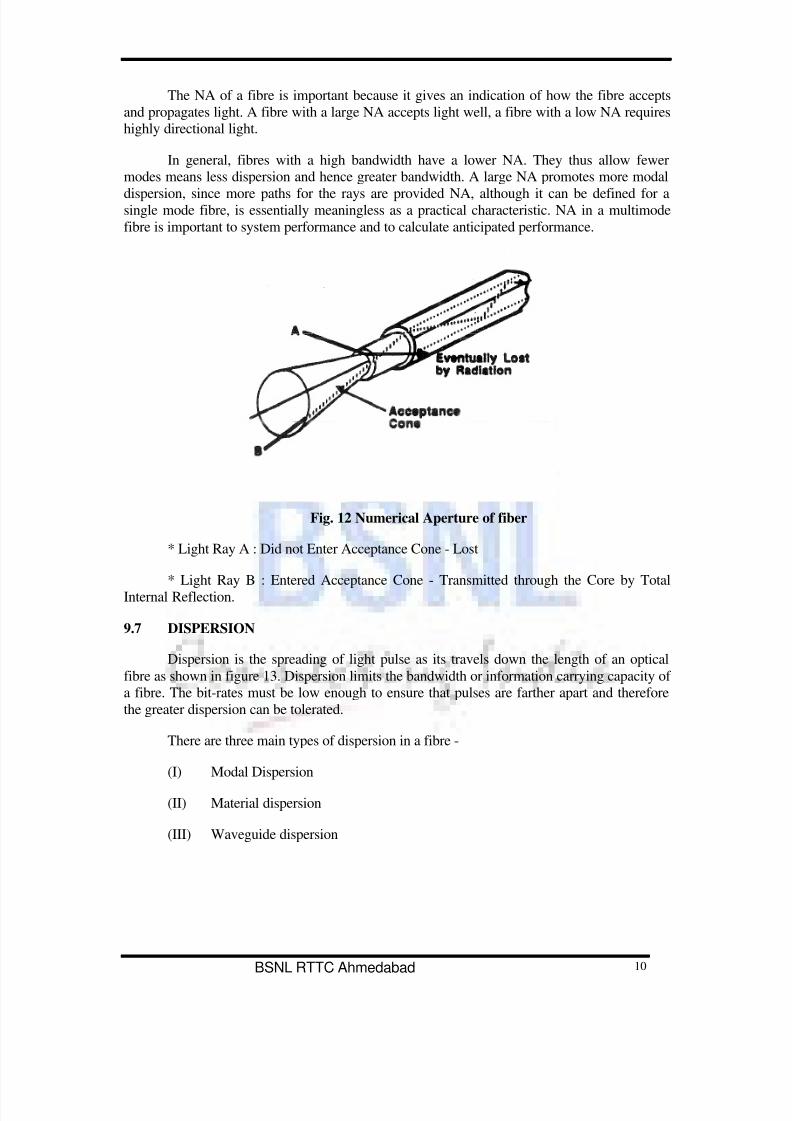
The NA of a fibre is important because it gives an indication of how the fibre accepts

and propagates light. A fibre with a large NA accepts light well, a fibre with a low NA requires

highly directional light.

In general, fibres with a high bandwidth have a lower NA. They thus allow fewer

modes means less dispersion and hence greater bandwidth. A large NA promotes more modal

dispersion, since more paths for the rays are provided NA, although it can be defined for asingle mode fibre, is essentially meaningless as a practical characteristic. NA in a multimode

fibre is important to system performance and to calculate anticipated performance.

Fig. 12 Numerical Aperture of fiber

* Light Ray A : Did not Enter Acceptance Cone - Lost

* Light Ray B : Entered Acceptance Cone - Transmitted through the Core by Total

Internal Reflection.

9.7 DISPERSION

Dispersion is the spreading of light pulse as its travels down the length of an optical

fibre as shown in figure 13. Dispersion limits the bandwidth or information carrying capacity of

a fibre. The bit-rates must be low enough to ensure that pulses are farther apart and therefore

the greater dispersion can be tolerated.

There are three main types of dispersion in a fibre -

(I) Modal Dispersion

(II) Material dispersion

(III) Waveguide dispersion




Fig. 13 Dispersion

9.8 BANDWIDTH AND DISPERSION :

A bandwidth of 400 MHz -km means that a 400 MHz-signal can be transmitted for 1

km. It means that the product of frequency and the length must be 400 or less. We can send a

lower frequency for a longer distance, i.e. 200 MHz for 2 km or 100 MHz for 4 km. Multimode

fibres are specified by the bandwidth-length product or simply bandwidth.

Single mode fibres on the other hand are specified by dispersion, expressed in

ps/km/nm. In other words for any given single mode fibre dispersion is most affected by the

source's spectral width. The wider the source spectral width, the greater the dispersion.

Conversion of dispersion to bandwidth can be approximated roughly by the following

equation.

0.187

BW = --------------------------

(Disp) (SW) (L)

Disp = Dispersion at the operating wavelength in seconds/ nm/ km.

SW = Spectral width of the source in nm.

L = Fibre length in km.

So the spectral width of the source has a significant effect on the performance of a

single mode fibre.

9.9 OPTICAL WINDOWS :

Attenuation of fibre for optical power varies with the wavelengths of light. Windows

are low-loss regions, where fiber carry light with little attenuation. The first generation of

optical fibre operated in the first window around 820 to 850 nm. The second window is the




zero-dispersion region of 1300 nm and the third window is the 1550 nm region as shown in

figure 14.

Fig. 14 Optical Windows

10.0 CABLE CONSTRUCTION

There are two basic cable designs are:

1. Tight Buffer Tube Cable

2. Loose Buffer Tube Cable

Loose-tube cable, used in the majority of outside-plant installations and tight-buffered

cable, primarily used inside buildings.

10.1 Tight-Buffered Cable

With tight-buffered cable designs, the buffering material is in direct contact with the

fiber. This design is suited for "jumper cables" which connect outside plant cables to terminal

equipment, and also for linking various devices in a premises network. Single-fiber tight-

buffered cables are used as pigtails, patch cords and jumpers to terminate loose-tube cables

directly into opto-electronic transmitters, receivers and other active and passive components.

Multi-fiber tight-buffered cables also are available and are used primarily for

alternative routing and handling flexibility and ease within buildings.The tight-buffered

design provides a rugged cable structure to protect individual fibers during handling, routing

and connectorization. Yarn strength members keep the tensile load away from the fiber.




Fig. 15 Tight Buffer Tube Cable

10.2 Loose-Tube Cable

The modular design of loose-tube cables typically holds 6, 12, 24, 48, 96 or evenmore than 400 fibers per cable. Loose-tube cables can be all-dielectric or optionally

armored. The loose-tube design also helps in the identification and administration of fibers in

the system.

In a loose-tube cable design, color-coded plastic buffer tubes house and protect

optical fibers. A gel filling compound impedes water penetration. Excess fiber length

(relative to buffer tube length) insulates fibers from stresses of installation and environmental

loading. Buffer tubes are stranded around a dielectric or steel central member, which serves

as an anti-buckling element.

The cable core, typically uses aramid yarn, as the primary tensile strength member.

The outer polyethylene jacket is extruded over the core. If armoring is required, a corrugatedsteel tape is formed around a single jacketed cable with an additional jacket extruded over the

armor.

Loose-tube cables typically are used for outside-plant installation in aerial, duct and

direct-buried applications.

Here are some common fiber cables types are given below:

10.2. 1 Distribution Cable

Distribution Cable (compact building cable) packages individual 900µm buffered

fiber reducing size and cost. The connectors may be installed directly on the 900µm bufferedfiber at the breakout box location.




Fig. 16 Distribution Cable

10.2.2 Loose Tube Cable

Loose tube cable is designed to endure outside temperatures and high moisture

conditions. The fibers are loosely packaged in gel filled buffer tubes to repel water.

Recommended for use between buildings that are unprotected from outside elements. Loose

tube cable is restricted from inside building use.

Fig.17 Loose Tube Cable

10.2.3 Aerial Cable/Self-Supporting

Aerial cable provides ease of installation and reduces time and cost. Figure 8 cable

can easily be separated between the fiber and the messenger. Temperature range (-55ºC to

+85ºC)

Fig. 18 Aerial Cable/Self-Supporting




10.2.4 Hybrid & Composite Cable

Hybrid cables offer the same great benefits as our standard indoor/outdoor cables, with

the convenience of installing multimode and single mode fibers all in one pull. Our

composite cables offer optical fiber along with solid 14 gauge wires suitable for a variety of

uses including power, grounding and other electronic controls

Fig. 19 Hybrid & Composite Cable

10.2.5 Armored Cable

Armored cable can be used for rodent protection in direct burial if required. This cable is

non-gel filled and can also be used in aerial applications. The armor can be removed leavingthe inner cable suitable for any indoor/outdoor use. (Temperature rating -40ºC to +85ºC)

Fig. 20 Armored Cable

Fibre Optic Cables (Loose Buffer Tube) have the following parts in common ;

(I) Optical Fibre

(II) Buffer

(III) Strength member

(IV) Jacket

Table-1 Cable Components

Component Function Material

Buffer Protect fibre From Outside Nylon, Mylar, Plastic

Central MemberFacilitate Stranding

Temperature StabilitySteel, Fibreglass




Anti-Buckling

Primary Strength

MemberTensile Strength Aramid Yarn, Steel

Cable Jacket

Contain and Protect

Cable Core

Abrasion Resistance

PE, PUR, PVC, Teflon

Cable Filling

Compound

Prevent Moisture

intrusion and Migration

Water Blocking

Compound

ArmoringRodent Protection

Crush Resistance

Steel Tape

11.0 CABLE DRUM LENGTH :

Cables come reeled in various length, typically 1 to 2 km, although lengths of 5 or 6

kms are available for single mode fibres. Long lengths are desirables for long distance

applications, since cable must be spliced end to end over the run. Each splice introduce

additional loss into the system. Long cable lengths mean fewer splices and less loss.

12.0 OFC Splicing

Splices are permanent connection between two fibres. The splicing involves cutting of

the edges of the two fibres to be spliced.

Splicing Methods

The following three types are widely used :

1. Adhesive bonding or Glue splicing.

2. Mechanical splicing.

3. Fusion splicing.

12.1 Adhesive Bonding or Glue Splicing

This is the oldest splicing technique used in fibre splicing. After fibre end preparation,

it is axially aligned in a precision V–groove. Cylindrical rods or another kind of reference

surfaces are used for alignment. During the alignment of fibre end, a small amount of

adhesive or glue of same refractive index as the core material is set between and around the

fibre ends. A two component epoxy or an UV curable adhesive is used as the bonding agent.

The splice loss of this type of joint is same or less than fusion splices. But fusion splicing

technique is more reliable, so at present this technique is very rarely used.




12.2 Mechanical Splicing

This technique is mainly used for temporary splicing in case of emergency repairing.

This method is also convenient to connect measuring instruments to bare fibres for taking

various measurements.

The mechanical splices consist of 4 basic components :

(i) An alignment surface for mating fibre ends.

(ii) A retainer

(iii) An index matching material.

(iv) A protective housing

A very good mechanical splice for M.M. fibres can have an optical performance as

good as fusion spliced fibre or glue spliced. But in case of single mode fibre, this type of

splice cannot have stability of loss.

12.3 Fusion Splicing

The fusion splicing technique is the most popular technique used for achieving very

low splice losses. The fusion can be achieved either through electrical arc or through gas

flame.

The process involves cutting of the fibres and fixing them in micro–positioners on the

fusion splicing machine. The fibres are then aligned either manually or automatically core

aligning (in case of S.M. fibre) process. Afterwards the operation that takes place involve

withdrawal of the fibres to a specified distance, preheating of the fibre ends through electric

arc and bringing together of the fibre ends in a position and splicing through high temperature

fusion.

If proper care taken and splicing is done strictly as per schedule, then the splicing loss

can be minimized as low as 0.01 dB/joint. After fusion splicing, the splicing joint should be

provided with a proper protector to have following protections:

(a) Mechanical protection

(b) Protection from moisture.

Sometimes the two types of protection are combined. Coating with Epoxy resins

protects against moisture and also provides mechanical strength at the joint.

Now–a–days, the heat shrinkable tubes are most widely used, which are fixed on the

joints by the fusion tools.

The fusion splicing technique is the most popular technique used for achieving very

low splice losses. The introduction of single mode optical fibre for use in long haul network

brought with it fibre construction and cable design different from those of multimode fibres.




The splicing machines imported by BSNL begins to the core profile alignment

system, the main functions of which are :

(1) Auto active alignment of the core.

(2) Auto arc fusion.

(3) Video display of the entire process.

(4) Indication of the estimated splice loss.

The two fibres ends to be spliced are cleaved and then clamped in accurately

machined vee–grooves. When the optimum alignment is achieved, the fibres are fused under

the microprocessor contorl, the machine then measures the radial and angular off–sets of the

fibres and uses these figures to calculate a splice loss. The operation of the machine observes

the alignment and fusion processes on a video screens showing horizontal and vertical

projection of the fibres and then decides the quality of the splice.

The splice loss indicated by the splicing machine should not be taken as a final value

as it is only an estimated loss and so after every splicing is over, the splice loss measurement

is to be taken by an OTDR (Optical Time Domain Reflectometer). The manual part of the

splicing is cleaning and cleaving the fibres. For cleaning the fibres, Dichlorine Methyl or

Acetone or Alcohol is used to remove primary coating.

With the special fibre cleaver or cutter, the cleaned fibre is cut. The cut has to be so

precise that it produces an end angle of less than 0.5 degree on a prepared fibre. If the cut is

bad, the splicing loss will increase or machine will not accept for splicing. The shape of the

cut can be monitored on the video screen, some of the defect noted while cleaving are listed

below :

(i) Broken ends.

(ii) Ripped ends.

(iii) Slanting cuts.

(iv) Unclean ends.

It is also desirable to limit the average splice loss to be less than 0.1 dB.




OF TRANSMISSION SYSTEMS & THEIR FEATURES

1.0 INTRODUCTION

With the introduction of PCM technology in the 1960s, communications networks

were gradually converted to digital technology over the next few years. To cope with the

demand for ever higher bit rates, a multiplex hierarchy called the plesiochronous digitalhierarchy (PDH) evolved. The bit rates start with the basic multiplex rate of 2 Mbit/s with

further stages of 8, 34 and 140 Mbit/s. In North America and Japan, the primary rate is 1.5

Mbit/s. Hierarchy stages of 6 and 44 Mbit/s developed from this. Because of these very

different developments, gateways between one network and another were very difficult and

expensive to realize. PCM allows multiple use of a single line by means of digital time-

domain multiplexing. The analog telephone signal is sampled at a bandwidth of 3.1 kHz,

quantized and encoded and then transmitted at a bit rate of 64 kbit/s. A transmission rate of

2048 kbit/s results when 30 such coded channels are collected together into a frame along

with the necessary signaling information. This so-called primary rate is used throughout the

world. Only the USA, Canada and Japan use a primary rate of 1544 kbit/s, formed by

combining 24 channels instead of 30. The growing demand for more bandwidth meant that

more stages of multiplexing were needed throughout the world. A practically synchronous

(or, to give it its proper name: plesiochronous) digital hierarchy is the result. Slight

differences in timing signals mean that justification or stuffing is necessary when forming the

multiplexed signals. Inserting or dropping an individual 64 kbit/s channel to or from a higher

digital hierarchy requires a considerable amount of complex multiplexer equipment.

Fig. 1 Plesiochronous Digital Hierarchies (PDH)

Traditionally, digital transmission systems and hierarchies have been based on

multiplexing signals which are plesiochronous (running at almost the same speed). Also,

various parts of the world use different hierarchies which lead to problems of international




interworking; for example, between those countries using 1.544 Mbit/s systems (U.S.A. and

Japan) and those using the 2.048 Mbit/s system. To recover a 64 kbit/s channel from a 140

Mbit/s PDH signal, it’s necessary to demultiplex the signal all the way down to the 2 Mbit/s

level before the location of the 64 kbit/s channel can be identified. PDH requires “steps”

(140-34, 34-8, 8-2 demultiplex; 2-8, 8-34, 34-140 multiplex) to drop out or add an individual

speech or data channel (see Figure 1).

The main problems of PDH systems are:

1. Homogeneity of equipment

2. Problem of Channel segregation

3. The problem cross connection of channels

4. Inability to identify individual channels in a higher-order bit stream.

5. Insufficient capacity for network management;

6. Most PDH network management is proprietary.

7. There’s no standardized definition of PDH bit rates greater than 140 Mb/s.

8. There are different hierarchies in use around the world. Specialized interface

equipment is required to interwork the two hierarchies.

1988 SDH standard introduced with three major goals:

– Avoid the problems of PDH

– Achieve higher bit rates (Gbit/s)

– Better means for Operation, Administration, and Maintenance (OA&M)

SDH is an ITU-T standard for a high capacity telecom network. SDH is a synchronous

digital transport system, aim to provide a simple, economical and flexible telecom

infrastructure. The basis of Synchronous Digital Hierarchy (SDH) is synchronous

multiplexing - data from multiple tributary sources is byte interleaved.

SDH brings the following advantages to network providers:

1.1 High transmission rates

Transmission rates of up to 40 Gbit/s can be achieved in modern SDH systems. SDH

is therefore the most suitable technology for backbones, which can be considered as being the

super highways in today's telecommunications networks.

1.2 Simplified add & drop function

Compared with the older PDH system, it is much easier to extract and insert low-bit

rate channels from or into the high-speed bit streams in SDH. It is no longer necessary to

demultiplex and then remultiplex the plesiochronous structure.




1.3 High availability and capacity matching

With SDH, network providers can react quickly and easily to the requirements of their

customers. For example, leased lines can be switched in a matter of minutes. The network

provider can use standardized network elements that can be controlled and monitored from a

central location by means of a telecommunications network management (TMN) system.

1.4 Reliability

Modern SDH networks include various automatic back-up and repair mechanisms to

cope with system faults. Failure of a link or a network element does not lead to failure of the

entire network which could be a financial disaster for the network provider. These back-up

circuits are also monitored by a management system.

1.5 Future-proof platform for new services

Right now, SDH is the ideal platform for services ranging from POTS, ISDN and

mobile radio through to data communications (LAN, WAN, etc.), and it is able to handle the

very latest services, such as video on demand and digital video broadcasting via ATM thatare gradually becoming established.

1.6 Interconnection

SDH makes it much easier to set up gateways between different network providers

and to SONET systems. The SDH interfaces are globally standardized, making it possible to

combine network elements from different manufacturers into a network. The result is a

reduction in equipment costs as compared with PDH.

2.0 Network Elements of SDH

Figure 2 is a schematic diagram of a SDH ring structure with various tributaries. The

mixture of different applications is typical of the data transported by SDH. Synchronous

networks must be able to transmit plesiochronous signals and at the same time be capable of

handling future services such as ATM.

Current SDH networks are basically made up from four different types of network

element. The topology (i.e. ring or mesh structure) is governed by the requirements of the

network provider.

2.1 Regenerators

Regenerators as the name implies, have the job of regenerating the clock and

amplitude relationships of the incoming data signals that have been attenuated and distorted

by dispersion. They derive their clock signals from the incoming data stream. Messages arereceived by extracting various 64 kbit/s channels (e.g. service channels E1, F1) in the RSOH

(regenerator section overhead). Messages can also be output using these channels.

2.2 Terminal Multiplexer

Terminal multiplexers Terminal multiplexers are used to combine plesiochronous and

synchronous input signals into higher bit rate STM-N signals.




Fig. 2 Schematic diagram of hybrid communications networks

2.3 Add/drop Multiplexers(ADM)

Add/drop multiplexers (ADM) Plesiochronous and lower bit rate synchronous signals

can be extracted from or inserted into high speed SDH bit streams by means of ADMs. This

feature makes it possible to set up ring structures, which have the advantage that automatic

back-up path switching is possible using elements in the ring in the event of a fault.

2.4 Digital Cross-connect

Digital cross-connects (DXC) This network element has the widest range of functions.

It allows mapping of PDH tributary signals into virtual containers as well as switching ofvarious containers up to and including VC-4.

2.5 Network Element Manager

Network element management The telecommunications management network (TMN)

is considered as a further element in the synchronous network. All the SDH network elements

mentioned so far are software-controlled. This means that they can be monitored and

remotely controlled, one of the most important features of SDH. Network management is

described in more detail in the section “TMN in the SDH network”

3.0 SDH Rates

SDH is a transport hierarchy based on multiples of 155.52 Mbit/s. The basic unit of

SDH is STM-1. Different SDH rates are given below:

STM-1 = 155.52 Mbit/s

STM-4 = 622.08 Mbit/s

STM-16 = 2588.32 Mbit/s




STM-64 = 9953.28 Mbit/s

Each rate is an exact multiple of the lower rate therefore the hierarchy is synchronous.

4.0 Back-up network switching- Automatic protection switching (APS)

Modern society is virtually completely dependent on communications technology.Trying to imagine a modern office without any connection to telephone or data networks is like

trying to work out how a laundry can operate without water. Network failures, whether due to

human error or faulty technology, can be very expensive for users and network providers alike.

As a result, the subject of so-called fall-back mechanisms is currently one of the most talked

about in the SDH world. A wide range of standardized mechanisms is incorporated into

synchronous networks in order to compensate for failures in network elements.

Two basic types of protection architecture are distinguished in APS. One is the linear

protection mechanism used for point-to-point connections. The other basic form is the so-called

ring protection mechanism which can take on many different forms. Both mechanisms use

spare circuits or components to provide the back-up path. Switching is controlled by the

overhead bytes K1 and K2.

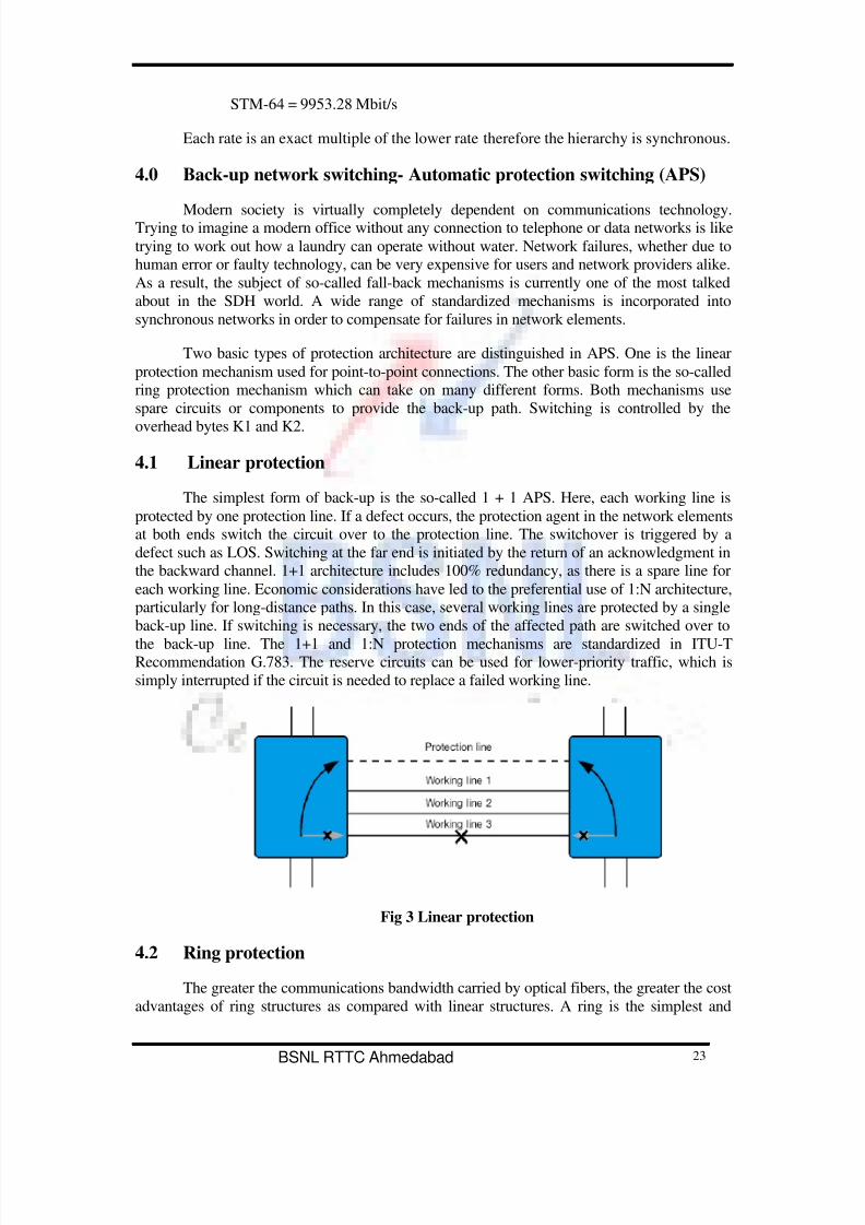
4.1 Linear protection

The simplest form of back-up is the so-called 1 + 1 APS. Here, each working line is

protected by one protection line. If a defect occurs, the protection agent in the network elements

at both ends switch the circuit over to the protection line. The switchover is triggered by a

defect such as LOS. Switching at the far end is initiated by the return of an acknowledgment in

the backward channel. 1+1 architecture includes 100% redundancy, as there is a spare line for

each working line. Economic considerations have led to the preferential use of 1:N architecture,

particularly for long-distance paths. In this case, several working lines are protected by a single

back-up line. If switching is necessary, the two ends of the affected path are switched over to

the back-up line. The 1+1 and 1:N protection mechanisms are standardized in ITU-TRecommendation G.783. The reserve circuits can be used for lower-priority traffic, which is

simply interrupted if the circuit is needed to replace a failed working line.

Fig 3 Linear protection

4.2 Ring protection

The greater the communications bandwidth carried by optical fibers, the greater the cost

advantages of ring structures as compared with linear structures. A ring is the simplest and




most cost-effective way of linking a number of network elements. Various protection

mechanisms are available for this type of network architecture, only some of which have been

standardized in ITU-T Recommendation G.841. A basic distinction must be made between ring

structures with unidirectional and bi-directional connections.

4.2.1 Unidirectional rings

Figure 4 shows the basic principle of APS for unidirectional rings. Let us assume that

there is an interruption in the circuit between the network elements A and B. Direction y is

unaffected by this fault. An alternative path must, however, be found for direction x.

Figure 4: Two fiber unidirectional path switched ring

The connection is therefore switched to the alternative path in network elements A and

B. The other network elements (C and D) switch through the back-up path. This switching

process is referred to as line switched. A simpler method is to use the so-called path switched

ring (see figure 4). Traffic is transmitted simultaneously over both the working line and the

protection line. If there is an interruption, the receiver (in this case A) switches to the protectionline and immediately takes up the connection.

4.2.2 Bi-directional rings

In this network structure, connections between network elements are bi-directional.

This is indicated in figure 5 by the absence of arrows when compared with figure 5. The overall

capacity of the network can be split up for several paths each with one bi-directional working

line, while for unidirectional rings, an entire virtual ring is required for each path. If a fault

occurs between neighboring elements A and B, network element B triggers protection

switching and controls network element A by means of the K1 and K2 bytes in the SOH.

Even greater protection is provided by bi-directional rings with 4 fibers. Each pair offibers transports working and protection channels. This results in 1:1 protection, i.e. 100 %

redundancy. This improved protection is coupled with relatively high costs.




Figure 5: Two fiber bi-directional line-switched ring (BLSR)

5. OFC & OFS Concepts

Documents

Transcript of 5. OFC & OFS Concepts