5 giugno 2012 Principali modifiche apportate alle nuove versioni
21
IJMMS 2004:11, 579–598 PII. S0161171204305260 http://ijmms.hindawi.com © Hindawi Publishing Corp. INTEGRAL TRANSFORMS, CONVOLUTION PRODUCTS, AND FIRST VARIATIONS BONG JIN KIM, BYOUNG SOO KIM, and DAVID SKOUG Received 21 May 2003 We establish the various relationships that exist among the integral transform α,β F , the convolution product (F ∗G) α , and the first variation δF for a class of functionals defined on K[0,T], the space of complex-valued continuous functions on [0,T] which vanish at zero. 2000 Mathematics Subject Classification: 28C20. 1. Introduction and definitions. In a unifying paper [10], Lee defined an integral transform α,β of analytic functionals on an abstract Wiener space. For certain values of the parameters α and β and for certain classes of functionals, the Fourier-Wiener transform [2], the Fourier-Feynman transform [3], and the Gauss transform are special cases of his integral transform α,β . In [5], Chang et al. established an interesting re- lationship between the integral transform and the convolution product for functionals on an abstract Wiener space. In this paper, we study the relationships that exist among the integral transform, the convolution product, and the first variation [1, 4, 9, 11]. Let C 0 [0,T] denote one-parameter Wiener space, that is, the space of all real-valued continuous functions x(t) on [0,T] with x(0) = 0. Let denote the class of all Wiener measurable subsets of C 0 [0,T] and let m denote Wiener measure. Then (C 0 [0,T], , m) is a complete measure space and we denote the Wiener integral of a Wiener inte- grable functional F by C 0 [0,T ] F(x)m(dx). (1.1) Let K = K[0,T] be the space of complex-valued continuous functions defined on [0,T] which vanish at t = 0. Let α and β be nonzero complex numbers. Next we state the definitions of the integral transform α,β F , the convolution product (F ∗ G) α , and the first variation δF for functionals defined on K. Definition 1.1. Let F be a functional defined on K. Then the integral transform α,β F of F is defined by α,β (F)(y) ≡ α,β F(y) ≡ C 0 [0,T ] F(αx + βy)m(dx), y ∈ K, (1.2) if it exists [5, 8, 10].
Transcript of 5 giugno 2012 Principali modifiche apportate alle nuove versioni
IJMMS 2004:11, 579–598PII. S0161171204305260
http://ijmms.hindawi.com© Hindawi Publishing Corp.
INTEGRAL TRANSFORMS, CONVOLUTION PRODUCTS,AND FIRST VARIATIONS
BONG JIN KIM, BYOUNG SOO KIM, and DAVID SKOUG
Received 21 May 2003
We establish the various relationships that exist among the integral transform �α,βF , theconvolution product (F∗G)α, and the first variation δF for a class of functionals defined onK[0,T ], the space of complex-valued continuous functions on [0,T ] which vanish at zero.
2000 Mathematics Subject Classification: 28C20.
1. Introduction and definitions. In a unifying paper [10], Lee defined an integral
transform �α,β of analytic functionals on an abstract Wiener space. For certain values
of the parameters α and β and for certain classes of functionals, the Fourier-Wiener
transform [2], the Fourier-Feynman transform [3], and the Gauss transform are special
cases of his integral transform �α,β. In [5], Chang et al. established an interesting re-
lationship between the integral transform and the convolution product for functionals
on an abstract Wiener space. In this paper, we study the relationships that exist among
the integral transform, the convolution product, and the first variation [1, 4, 9, 11].
Let C0[0,T ] denote one-parameter Wiener space, that is, the space of all real-valued
continuous functions x(t) on [0,T ] with x(0)= 0. Let � denote the class of all Wiener
measurable subsets of C0[0,T ] and let m denote Wiener measure. Then (C0[0,T ],�,m) is a complete measure space and we denote the Wiener integral of a Wiener inte-
grable functional F by
∫C0[0,T ]
F(x)m(dx). (1.1)
Let K = K[0,T ] be the space of complex-valued continuous functions defined on
[0,T ] which vanish at t = 0. Let α and β be nonzero complex numbers. Next we state
the definitions of the integral transform �α,βF , the convolution product (F∗G)α, and
the first variation δF for functionals defined on K.
Definition 1.1. Let F be a functional defined on K. Then the integral transform
�α,βF of F is defined by
�α,β(F)(y)≡�α,βF(y)≡∫C0[0,T ]
F(αx+βy)m(dx), y ∈K, (1.2)
if it exists [5, 8, 10].
580 BONG JIN KIM ET AL.
Definition 1.2. Let F and G be functionals defined on K. Then the convolution
product (F∗G)α of F and G is defined by
(F∗G)α(y)≡∫C0[0,T ]
F(y+αx√
2
)G(y−αx√
2
)m(dx), y ∈K, (1.3)
if it exists [5, 7, 13, 14].
Definition 1.3. Let F be a functional defined on K and let w ∈ K. Then the first
variation δF of F is defined by
δF(y|w)≡ ∂∂tF(y+tw)|t=0, y ∈K, (1.4)
if it exists [1, 4, 11].
Let {θ1,θ2, . . .} be a complete orthonormal set of real-valued functions in L2[0,T ].Furthermore, assume that each θj is of bounded variation on [0,T ]. Also let Var(θj,[0,T ]) denote the total variation of θj on [0,T ]. Then for each y ∈ K and j ∈ {1,2, . . .},the Riemann-Stieltjes integral 〈θj,y〉 ≡
∫ T0 θj(t)dy(t) exists. Furthermore,
∣∣⟨θj,y⟩∣∣=∣∣∣∣θj(T)y(T)−
∫ T0y(t)dθj(t)
∣∣∣∣≤ Cj‖y‖∞ (1.5)
with
Cj =∣∣θj(T)∣∣+Var
(θj,[0,T ]
). (1.6)
Next we describe the class of functionals that we work with in this paper. Let E0 be
the space of all functionals F :K→ C of the form
F(y)= f (⟨θ1,y⟩, . . . ,
⟨θn,y
⟩)(1.7)
for some positive integer n, where f(λ1, . . . ,λn) is an entire function of the n complex
variables λ1, . . . ,λn of exponential type; that is to say,
∣∣f (λ1, . . . ,λn)∣∣≤AF exp
BF
n∑j=1
∣∣λj∣∣ (1.8)
for some positive constants AF and BF .
To simplify the expressions, we use the following notations. For �u= (u1, . . . ,un)∈Rnand �λ= (λ1, . . . ,λn)∈ Cn, we write
‖�u‖2 =n∑j=1
u2j , |�u| =
n∑j=1
∣∣uj∣∣, |�λ| =n∑j=1
∣∣λj∣∣, d�u= du1 ···dun,
f(α�u+β�λ)= f (αu1+βλ1, . . . ,αun+βλn
),
f(⟨�θ,y⟩)= f (⟨θ1,y
⟩, . . . ,
⟨θn,y
⟩).
(1.9)
INTEGRAL TRANSFORMS, CONVOLUTION PRODUCTS, . . . 581
Hence (1.7) and (1.8) can be expressed alternatively as
F(y)= f (〈�θ,y〉), ∣∣f(�λ)∣∣≤AF exp{BF |�λ|
}, (1.10)
respectively. In addition, we use the notation
Fj(y)= fj(〈�θ,y〉), (1.11)
where fj(�λ)= (∂/∂λj)f (λ1, . . . ,λn) for j = 1, . . . ,n.
In Section 2, we show that if F and G are elements of E0, then �α,βF(·), (F∗G)α(·),δF(·|w), and δF(y|·) are also elements of E0. In Section 3, we examine all relationships
involving exactly two of the three concepts of “integral transform,” “convolution prod-
uct,” and “first variation,” while in Section 4, we examine all relationships involving all
three of these concepts where each concept is used exactly once. For related work, see
[2, 5, 7, 9, 10, 11, 13, 14] and for a detailed survey of previous work, see [12].
Remark 1.4. For any F ∈ E0 and any G ∈ E0, we can always express F by (1.7) and
G by
G(x)= g(⟨θ1,x⟩, . . . ,
⟨θn,x
⟩)(1.12)
using the same positive integer n, where f and g are entire functions of exponential
type. For example, if F ∈ E0 is of the form
F(x)= r(⟨θ1,x⟩,⟨θ2,x
⟩), (1.13)
and G ∈ E0 is of the form
G(x)= s(⟨θ1,x⟩,⟨θ3,x
⟩,⟨θ4,x
⟩), (1.14)
where r(λ1,λ2) and s(λ1,λ3,λ4) are entire functions of exponential type, then we can
express F and G by (1.7) and (1.12) with n= 4 by choosing f(λ1,λ2,λ3,λ4)≡ r(λ1,λ2)and g(λ1,λ2,λ3,λ4) ≡ s(λ1,λ3,λ4). In addition, the positive constants AF , BF , AG, and
BG remain fixed. Thus throughout this paper, we will always assume that F andG belong
to E0 and are given by (1.7) and (1.12), respectively.
Remark 1.5. We considered various other classes of functionals before deciding to
work exclusively with the class E0 throughout this paper. One very natural class we
considered was L2(C) ≡ L2(C0[0,T ]), the space of all complex-valued functionals Fsatisfying
∫C0[0,T ]
∣∣F(x)∣∣2m(dx) <∞. (1.15)
However in [8], Kim and Skoug showed that L2(C) is not invariant under the action of
the integral transform operator. In fact, they showed that for every β∈ C with |β|> 1,
there exists a functional F ∈ L2(C) (the functional F depends on β) with �α,β(F) ∉ L2(C)even though α2+β2 = 1.

582 BONG JIN KIM ET AL.
Another class of functionals we considered was
A= {F ∈ L2(C) : �α,β(F)∈ L2(C) ∀ nonzero α,β∈ C}. (1.16)
But for F ∈A, the first variation δF of F may not exist; in fact, one needs some kind of
a smoothness condition on F to even define δF .
As we will see in Section 2, E0 is a very natural class of functionals in which to study
the relationships that exist among the integral transform, the convolution product, and
the first variation because for F and G in E0, �α,β(F) and (F∗G)α exist and belong to
E0 for all nonzero complex numbers α and β, while δF(y|w) exists and belongs to E0
for all y and w in K. In addition, E0 is a very rich class of functionals. Note that if
E0 is given by (1.7), then the entire function f(λ1, . . . ,λn) is bounded if and only if it
is a constant function. Thus many of the functionals in E0 are unbounded, while for
example, all of the functionals considered in [11] are bounded.
The so-called “tame functionals,” that is, functionals of the form
G(x)= g(x(t1), . . . ,x(tm)), 0< t1 < ···< tm ≤ T (1.17)
as well as functionals of the form (1.7), played a major role in the development of
Wiener space integration theory. But functionals of the form (1.17) are in E0 provided
g(λ1, . . . ,λm) is an entire function of exponential growth. Included of course are all
polynomials of m complex variables λ1, . . . ,λm for all positive integers m, as well as
such polynomials in x(t1), . . . ,x(tm) multiplied by functionals like exp{∑mj=1ajxj(t)},
and so forth.
2. The integral transform, the convolution product, and the first variation of func-
tionals in E0. In our first theorem, we show that if F is an element of E0, then the
integral transform of F exists and is an element of E0.
Theorem 2.1. Let F ∈ E0 be given by (1.7). Then the integral transform �α,βF exists,
belongs to E0, and is given by the formula
�α,βF(y)= h(〈�θ,y〉) (2.1)
for y ∈K, where
h(�λ)= (2π)−n/2∫Rnf (α�u+β�λ)exp
{− 1
2‖�u‖2
}d�u. (2.2)
Proof. For each y ∈K, using a well-known Wiener integration theorem, we obtain
�α,βF(y)=∫C0[0,T ]
f(α〈�θ,x〉+β〈�θ,y〉)m(dx)
= (2π)−n/2∫Rnf(α�u+β〈�θ,y〉)exp
{− 1
2‖�u‖2
}d�u
= h(〈�θ,y〉),(2.3)
INTEGRAL TRANSFORMS, CONVOLUTION PRODUCTS, . . . 583
where h is given by (2.2). By [6, Theorem 3.15], h(�λ) is an entire function. Moreover, by
inequality (1.8), we have
∣∣h(�λ)∣∣≤ (2π)−n/2∫RnAF exp
{BF |α�u+β�λ|− 1
2‖�u‖2
}d�u
≤A�α,βF exp{B�α,βF |�λ|
},
(2.4)
where
A�α,βF =AF(
1√2π
∫R
exp{− u
2
2+BF |αu|
}du
)n<∞ (2.5)
and B�α,βF = BF |β|. Hence �α,βF ∈ E0.
In our next theorem, we show that the convolution product of functionals from E0 is
an element of E0.
Theorem 2.2. Let F,G ∈ E0 be given by (1.7) and (1.12) with corresponding entire
functions f and g. Then the convolution (F ∗G)α exists, belongs to E0, and is given by
the formula
(F∗G)α(y)= k(〈�θ,y〉) (2.6)
for y ∈K, where
k(�λ)= (2π)−n/2
∫Rnf(�λ+α�u√
2
)g(�λ−α�u√
2
)exp
{− 1
2‖�u‖2
}d�u. (2.7)
Proof. For each y ∈K, using a well-known Wiener integration theorem, we obtain
(F∗G)α(y)=∫C0[0,T ]
F(y+αx√
2
)G(y−αx√
2
)m(dx)
=∫C0[0,T ]
f(〈�θ,y〉+α〈�θ,x〉√
2
)g(〈�θ,y〉−α〈�θ,x〉√
2
)m(dx)
= (2π)−n/2∫Rnf(〈�θ,y〉+α�u√
2
)g(〈�θ,y〉−α�u√
2
)exp
{− 1
2‖�u‖2
}d�u
= k(〈�θ,y〉),
(2.8)
where k is given by (2.7). By [6, Theorem 3.15], k(�λ) is an entire function and
∣∣k(�λ)∣∣≤ (2π)−n/2∫RnAFAG exp
{BF +BG√
2
(|�λ|+|α||�u|)− 12‖�u‖2
}d�u
=A(F∗G)α exp{B(F∗G)α |�λ|
},
(2.9)
where B(F∗G)α = (BF +BG)/√
2 and
A(F∗G)α =AFAG(
1√2π
∫R
exp{− u
2
2+B(F∗G)α |αu|
}du
)n<∞. (2.10)
Hence (F∗G)α ∈ E0.
584 BONG JIN KIM ET AL.
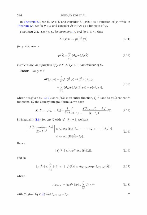
In Theorem 2.3, we fix w ∈ K and consider δF(y|w) as a function of y , while in
Theorem 2.4, we fix y ∈K and consider δF(y|w) as a function of w.
Theorem 2.3. Let F ∈ E0 be given by (1.7) and let w ∈K. Then
δF(y|w)= p(〈�θ,y〉) (2.11)
for y ∈K, where
p(�λ)=n∑j=1
⟨θj,w
⟩fj(�λ). (2.12)
Furthermore, as a function of y ∈K, δF(y|w) is an element of E0.
Proof. For y ∈K,
δF(y|w)= ∂∂tf(〈�θ,y〉+t〈�θ,w〉)∣∣t=0
=n∑j=1
⟨θj,w
⟩fj(〈�θ,y〉)= p(〈�θ,y〉), (2.13)
where p is given by (2.12). Since f(�λ) is an entire function, fj(�λ) and so p(�λ) are entire
functions. By the Cauchy integral formula, we have
fj(λ1, . . . ,λj, . . . ,λn
)= 12πi
∫|ζ−λj |=1
f(λ1, . . . ,ζ, . . . ,λn
)(ζ−λj
)2 dζ. (2.14)
By inequality (1.8), for any ζ with |ζ−λj| = 1, we have
∣∣∣∣∣f(λ1, . . . ,ζ, . . . ,λn
)(ζ−λj
)2
∣∣∣∣∣≤AF exp{BF(∣∣λ1
∣∣+···+|ζ|+···+∣∣λn∣∣)}
≤AF exp{BF |�λ|+BF
}.
(2.15)
Hence
∣∣fj(�λ)∣∣≤AFeBF exp{BF |�λ|
}, (2.16)
and so
∣∣p(�λ)∣∣≤ n∑j=1
∣∣⟨θj,w⟩∣∣∣∣fj(�λ)∣∣≤AδF(·|w) exp{BδF(·|w)|�λ|
}, (2.17)
where
AδF(·|w) =AFeBF ‖w‖∞n∑j=1
Cj <∞ (2.18)
with Cj given by (1.6) and BδF(·|w) = BF .
INTEGRAL TRANSFORMS, CONVOLUTION PRODUCTS, . . . 585
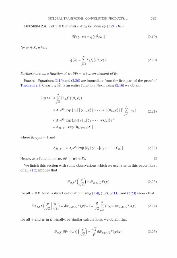
Theorem 2.4. Let y ∈K and let F ∈ E0 be given by (1.7). Then
δF(y|w)= q(〈�θ,w〉) (2.19)
for w ∈K, where
q(�λ)=n∑j=1
λjfj(〈�θ,y〉). (2.20)
Furthermore, as a function of w, δF(y|w) is an element of E0.
Proof. Equations (2.19) and (2.20) are immediate from the first part of the proof of
Theorem 2.3. Clearly q(�λ) is an entire function. Next, using (2.16) we obtain
∣∣q(�λ)∣∣≤ n∑j=1
∣∣λjfj(〈�θ,y〉)∣∣
≤AFeBF exp{BF[∣∣⟨θ1,y
⟩∣∣+···+∣∣⟨θn,y⟩∣∣]}n∑j=1
∣∣λj∣∣<AFeBF exp
{BF‖y‖∞
[C1+···+Cn
]}e|�λ|
=AδF(y|·) exp{BδF(y|·)|�λ|
},
(2.21)
where BδF(y|·) = 1 and
AδF(y|·) =AFeBF exp{BF‖y‖∞
[C1+···+Cn
]}. (2.22)
Hence, as a function of w, δF(y|w)∈ E0.
We finish this section with some observations which we use later in this paper. First
of all, (1.2) implies that
�α,βF(y√2
)=�α,β/
√2F(y) (2.23)
for all y ∈K. Next, a direct calculation using (1.4), (1.2), (2.11), and (2.23) shows that
δ�α,βF(y√2
∣∣∣∣ w√2
)= δ�α,β/
√2F(y|w)=
β√2
n∑j=1
⟨θj,w
⟩�α,β/
√2Fj(y) (2.24)
for all y and w in K. Finally, by similar calculations, we obtain that
�α,β(δF(·|w))( y√
2
)=√
2βδ�α,β/
√2F(y|w) (2.25)

586 BONG JIN KIM ET AL.
for all y and w in K, and for all y ∈K,
(�α,βF
)j(y)= β�α,β
(Fj)(y)= β�α,βFj(y). (2.26)
3. Relationships involving two concepts. In this section, we establish all of the
various relationships involving exactly two of the three concepts of integral transform,
convolution product, and first variation for functionals belonging to E0. The seven dis-
tinct relationships, as well as alternative expressions for some of them, are given by
(3.1), (3.2), (3.4), (3.7), (3.9), (3.11), and (3.13).
In view of Theorem 2.1 through Theorem 2.4, all of the functionals that occur in this
section are elements of E0. For example, let F and G be any functionals in E0. Then
by Theorem 2.2, the functional (F∗G)α belongs to E0, and hence by Theorem 2.1, the
functional �α,β(F∗G)α also belongs to E0. By similar arguments, all of the functionals
that arise in (3.1) through (3.14) and (3.16) through (3.20) exist and belong to E0.
Our first formula (3.1) is useful because it permits one to calculate �α,β(F ∗G)αwithout ever actually calculating (F∗G)α.
Formula 3.1. The integral transform of the convolution product of functionals
from E0 is given by the formula
�α,β(F∗G)α(y)=�α,βF(y√2
)�α,βG
(y√2
)=�α,β/
√2F(y)�α,β/
√2G(y) (3.1)
for all y in K.
Proof. Formula 3.1 is a special case of [5, Theorem 3.1].
Formula 3.2. The convolution product of the integral transform of functionals
from E0 is given by the formula
(�α,βF∗�α,βG
)α(y)
= (2π)−3n/2∫R3n
f(α�r + β√
2〈�θ,y〉+ βα√
2�u)
·g(α�s+ β√
2〈�θ,y〉− βα√
2�u)
exp
{− ‖�u‖
2+‖�r‖2+‖�s‖2
2
}d�ud�r d�s
(3.2)
for all y in K.
Proof. Using (1.3) and (1.2), we see that
(�α,βF∗�α,βG
)α(y)
=∫C0[0,T ]
�α,βF(y+αx√
2
)�α,βG
(y−αx√
2
)m(dx)
=∫C0[0,T ]
[∫C0[0,T ]
F(αz1+ β(y+αx)√
2
)m(dz1
)]
INTEGRAL TRANSFORMS, CONVOLUTION PRODUCTS, . . . 587
·[∫
C0[0,T ]G(αz2+ β(y−αx)√
2
)m(dz2
)]m(dx)
=∫C3
0 [0,T ]f(α⟨�θ,z1
⟩+ β√2〈�θ,y〉+ αβ√
2〈�θ,x〉
)
·g(α⟨�θ,z2
⟩+ β√2〈�θ,y〉− αβ√
2〈�θ,x〉
)m(dx)m
(dz1
)m(dz2
).
(3.3)
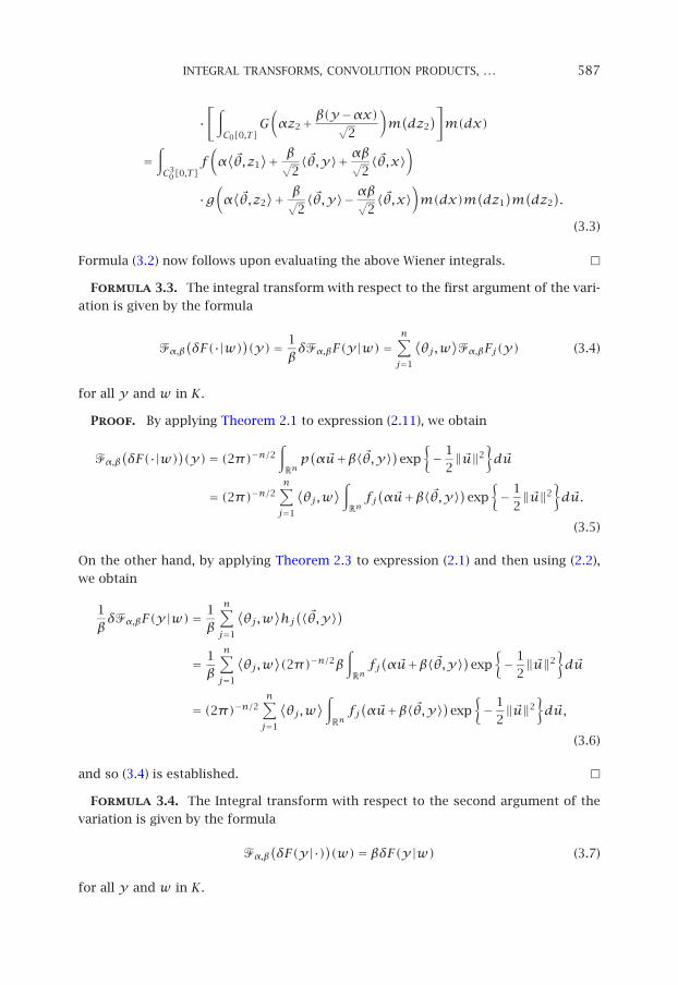
Formula (3.2) now follows upon evaluating the above Wiener integrals.
Formula 3.3. The integral transform with respect to the first argument of the vari-
ation is given by the formula
�α,β(δF(·|w))(y)= 1
βδ�α,βF(y|w)=
n∑j=1
⟨θj,w
⟩�α,βFj(y) (3.4)
for all y and w in K.
Proof. By applying Theorem 2.1 to expression (2.11), we obtain
�α,β(δF(·|w))(y)= (2π)−n/2
∫Rnp(α�u+β〈�θ,y〉)exp
{− 1
2‖�u‖2
}d�u
= (2π)−n/2n∑j=1
⟨θj,w
⟩∫Rnfj(α�u+β〈�θ,y〉)exp
{− 1
2‖�u‖2
}d�u.
(3.5)
On the other hand, by applying Theorem 2.3 to expression (2.1) and then using (2.2),
we obtain
1βδ�α,βF(y|w)= 1
β
n∑j=1
⟨θj,w
⟩hj(〈�θ,y〉)
= 1β
n∑j=1
⟨θj,w
⟩(2π)−n/2β
∫Rnfj(α�u+β〈�θ,y〉)exp
{− 1
2‖�u‖2
}d�u
= (2π)−n/2n∑j=1
⟨θj,w
⟩∫Rnfj(α�u+β〈�θ,y〉)exp
{− 1
2‖�u‖2
}d�u,
(3.6)
and so (3.4) is established.
Formula 3.4. The Integral transform with respect to the second argument of the
variation is given by the formula
�α,β(δF(y|·))(w)= βδF(y|w) (3.7)
for all y and w in K.
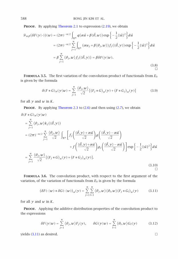
588 BONG JIN KIM ET AL.
Proof. By applying Theorem 2.1 to expression (2.19), we obtain
�α,β(δF(y|·))(w)= (2π)−n/2
∫Rnq(α�u+β〈�θ,w〉)exp
{− 1
2‖�u‖2
}d�u
= (2π)−n/2n∑j=1
∫Rn
(αuj+β
⟨θj,w
⟩)fj(〈�θ,y〉)exp
{− 1
2‖�u‖2
}d�u
= βn∑j=1
⟨θj,w
⟩fj(〈�θ,y〉)= βδF(y|w).
(3.8)
Formula 3.5. The first variation of the convolution product of functionals from E0
is given by the formula
δ(F∗G)α(y|w)=n∑j=1
⟨θj,w
⟩√
2
[(Fj∗G
)α(y)+
(F∗Gj
)α(y)
](3.9)
for all y and w in K.
Proof. By applying Theorem 2.3 to (2.6) and then using (2.7), we obtain
δ(F∗G)α(y|w)
=n∑j=1
⟨θj,w
⟩kj(〈�θ,y〉)
= (2π)−n/2n∑j=1
⟨θj,w
⟩√
2
∫Rn
[fj
(〈�θ,y〉+α�u√
2
)g(〈�θ,y〉−α�u√
2
)
+f(〈�θ,y〉+α�u√
2
)gj
(〈�θ,y〉−α�u√
2
)]exp
{− 1
2‖�u‖2
}d�u
=n∑j=1
⟨θj,w
⟩√
2
[(Fj∗G
)α(y)+
(F∗Gj
)α(y)
].
(3.10)
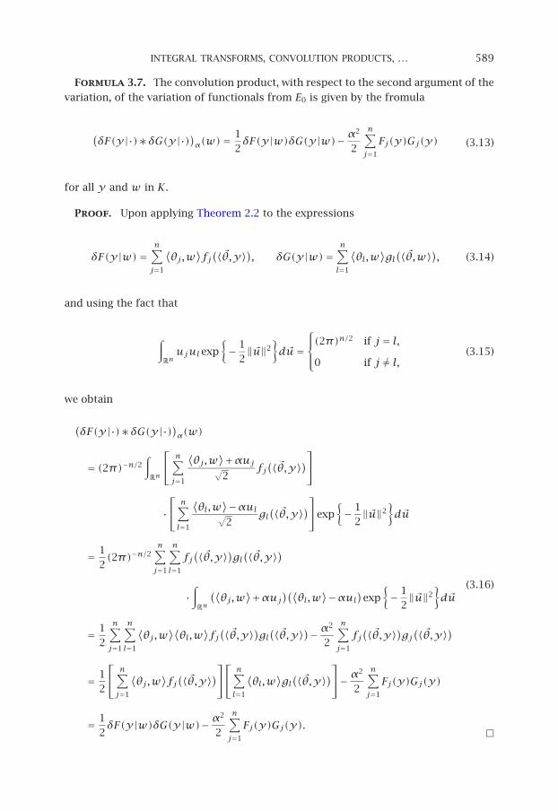
Formula 3.6. The convolution product, with respect to the first argument of the
variation, of the variation of functionals from E0 is given by the formula
(δF(·|w)∗δG(·|w))α(y)=
n∑j=1
n∑l=1
⟨θj,w
⟩⟨θl,w
⟩(Fj∗Gl
)α(y) (3.11)
for all y and w in K.
Proof. Applying the additive distribution properties of the convolution product to
the expressions
δF(y|w)=n∑j=1
⟨θj,w
⟩Fj(y), δG(y|w)=
n∑l=1
⟨θl,w
⟩Gl(y) (3.12)
yields (3.11) as desired.
INTEGRAL TRANSFORMS, CONVOLUTION PRODUCTS, . . . 589
Formula 3.7. The convolution product, with respect to the second argument of the
variation, of the variation of functionals from E0 is given by the fromula
(δF(y|·)∗δG(y|·))α(w)= 1
2δF(y|w)δG(y|w)− α
2
2
n∑j=1
Fj(y)Gj(y) (3.13)
for all y and w in K.
Proof. Upon applying Theorem 2.2 to the expressions
δF(y|w)=n∑j=1
⟨θj,w
⟩fj(〈�θ,y〉), δG(y|w)=
n∑l=1
⟨θl,w
⟩gl(〈�θ,w〉), (3.14)
and using the fact that
∫Rnujul exp
{− 1
2‖�u‖2
}d�u=
(2π)n/2 if j = l,0 if j �= l,
(3.15)
we obtain
(δF(y|·)∗δG(y|·))α(w)
= (2π)−n/2∫Rn
n∑j=1
⟨θj,w
⟩+αuj√2
fj(〈�θ,y〉)
· n∑l=1
⟨θl,w
⟩−αul√2
gl(〈�θ,y〉)
exp
{− 1
2‖�u‖2
}d�u
= 12(2π)−n/2
n∑j=1
n∑l=1
fj(〈�θ,y〉)gl(〈�θ,y〉)
·∫Rn
(⟨θj,w
⟩+αuj)(⟨θl,w⟩−αul)exp{− 1
2‖�u‖2
}d�u
= 12
n∑j=1
n∑l=1
⟨θj,w
⟩⟨θl,w
⟩fj(〈�θ,y〉)gl(〈�θ,y〉)− α2
2
n∑j=1
fj(〈�θ,y〉)gj(〈�θ,y〉)
= 12
n∑j=1
⟨θj,w
⟩fj(〈�θ,y〉)
n∑l=1
⟨θl,w
⟩gl(〈�θ,y〉)
− α2
2
n∑j=1
Fj(y)Gj(y)
= 12δF(y|w)δG(y|w)− α
2
2
n∑j=1
Fj(y)Gj(y).
(3.16)
590 BONG JIN KIM ET AL.
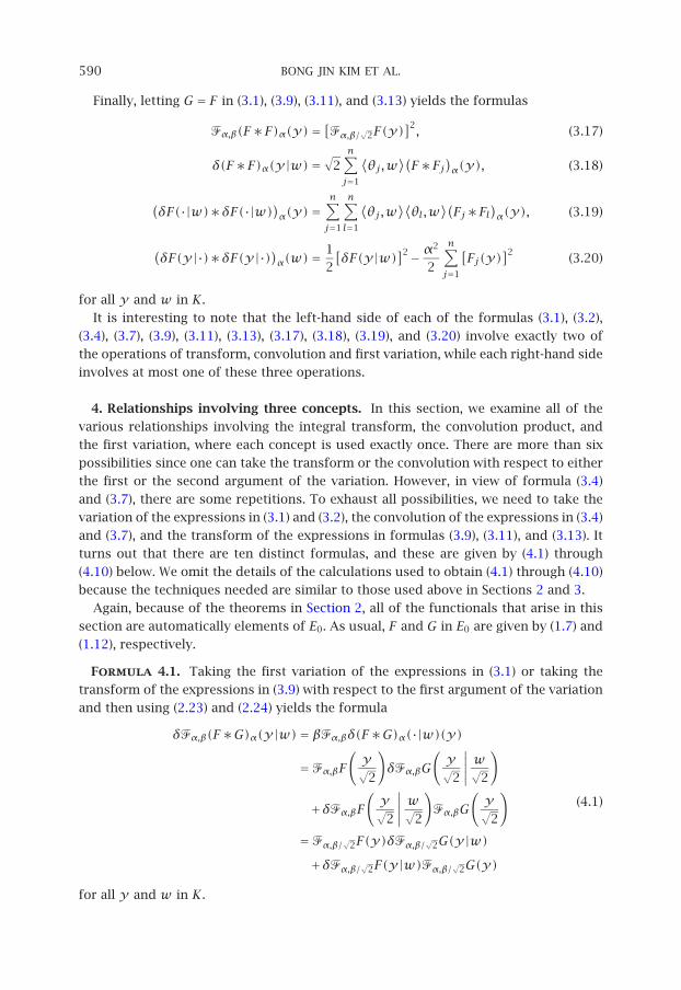
Finally, letting G = F in (3.1), (3.9), (3.11), and (3.13) yields the formulas
�α,β(F∗F)α(y)=[�α,β/
√2F(y)
]2, (3.17)
δ(F∗F)α(y|w)=√
2n∑j=1
⟨θj,w
⟩(F∗Fj
)α(y), (3.18)
(δF(·|w)∗δF(·|w))α(y)=
n∑j=1
n∑l=1
⟨θj,w
⟩⟨θl,w
⟩(Fj∗Fl
)α(y), (3.19)
(δF(y|·)∗δF(y|·))α(w)= 1
2
[δF(y|w)]2− α
2
2
n∑j=1
[Fj(y)
]2(3.20)
for all y and w in K.
It is interesting to note that the left-hand side of each of the formulas (3.1), (3.2),
(3.4), (3.7), (3.9), (3.11), (3.13), (3.17), (3.18), (3.19), and (3.20) involve exactly two of
the operations of transform, convolution and first variation, while each right-hand side
involves at most one of these three operations.
4. Relationships involving three concepts. In this section, we examine all of the
various relationships involving the integral transform, the convolution product, and
the first variation, where each concept is used exactly once. There are more than six
possibilities since one can take the transform or the convolution with respect to either
the first or the second argument of the variation. However, in view of formula (3.4)
and (3.7), there are some repetitions. To exhaust all possibilities, we need to take the
variation of the expressions in (3.1) and (3.2), the convolution of the expressions in (3.4)
and (3.7), and the transform of the expressions in formulas (3.9), (3.11), and (3.13). It
turns out that there are ten distinct formulas, and these are given by (4.1) through
(4.10) below. We omit the details of the calculations used to obtain (4.1) through (4.10)
because the techniques needed are similar to those used above in Sections 2 and 3.
Again, because of the theorems in Section 2, all of the functionals that arise in this
section are automatically elements of E0. As usual, F and G in E0 are given by (1.7) and
(1.12), respectively.
Formula 4.1. Taking the first variation of the expressions in (3.1) or taking the
transform of the expressions in (3.9) with respect to the first argument of the variation
and then using (2.23) and (2.24) yields the formula
δ�α,β(F∗G)α(y|w)= β�α,βδ(F∗G)α(·|w)(y)
=�α,βF(y√2
)δ�α,βG
(y√2
∣∣∣∣∣ w√2
)
+δ�α,βF(y√2
∣∣∣∣∣ w√2
)�α,βG
(y√2
)
=�α,β/√
2F(y)δ�α,β/√
2G(y|w)+δ�α,β/
√2F(y|w)�α,β/
√2G(y)
(4.1)
for all y and w in K.
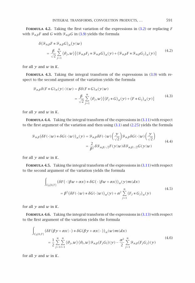
INTEGRAL TRANSFORMS, CONVOLUTION PRODUCTS, . . . 591
Formula 4.2. Taking the first variation of the expressions in (3.2) or replacing Fwith �α,βF and G with �α,βG in (3.9) yields the formula
δ(�α,βF∗�α,βG
)α(y|w)
= β√2
n∑j=1
⟨θj,w
⟩[(�α,βFj∗�α,βG
)α(y)+
(�α,βF∗�α,βGj
)α(y)
] (4.2)
for all y and w in K.
Formula 4.3. Taking the integral transform of the expressions in (3.9) with re-
spect to the second argument of the variation yields the formula
�α,βδ(F∗G)α(y|·)(w)= βδ(F∗G)α(y|w)
= β√2
n∑j=1
⟨θj,w
⟩[(Fj∗G
)α(y)+
(F∗Gj
)α(y)
] (4.3)
for all y and w in K.
Formula 4.4. Taking the integral transform of the expressions in (3.11) with respect
to the first argument of the variation and then using (3.1) and (2.25) yields the formula
�α,β(δF(·|w)∗δG(·|w))α(y)=�α,βδF(·|w)
(y√2
)�α,βδG(·|w)
(y√2
)
= 2β2δ�α,β/
√2F(y|w)δ�α,β/
√2G(y|w)
(4.4)
for all y and w in K.
Formula 4.5. Taking the integral transform of the expressions in (3.11) with respect
to the second argument of the variation yields the formula
∫C0[0,T ]
(δF(·|βw+αx)∗δG(·|βw+αx))α(y)m(dx)
= β2(δF(·|w)∗δG(·|w))α(y)+α2n∑j=1
(Fj∗Gj
)α(y)
(4.5)
for all y and w in K.
Formula 4.6. Taking the integral transform of the expressions in (3.13) with respect
to the first argument of the variation yields the formula
∫C0[0,T ]
(δF(βy+αx|·)∗δG(βy+αx|·))α(w)m(dx)
= 12
n∑j=1
n∑l=1
⟨θj,w
⟩⟨θl,w
⟩�α,β
(FjGl
)(y)− α
2
2
n∑j=1
�α,β(FjGj
)(y)
(4.6)
for all y and w in K.
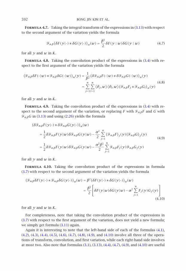
592 BONG JIN KIM ET AL.
Formula 4.7. Taking the integral transform of the expressions in (3.13) with respect
to the second argument of the variation yields the formula
�α,β(δF(y|·)∗δG(y|·))α(w)= β2
2δF(y |w)δG(y |w) (4.7)
for all y and w in K.
Formula 4.8. Taking the convolution product of the expressions in (3.4) with re-
spect to the first argument of the variation yields the formula
(�α,βδF(·|w)∗�α,βδG(·|w)
)α(y)=
1β2
(δ�α,βF(·|w)∗δ�α,βG(·|w)
)α(y)
=n∑j=1
n∑l=1
⟨θj,w
⟩⟨θl,w
⟩(�α,βFj∗�α,βGl
)α(y)
(4.8)
for all y and w in K.
Formula 4.9. Taking the convolution product of the expressions in (3.4) with re-
spect to the second argument of the variation, or replacing F with �α,βF and G with
�α,βG in (3.13) and using (2.26) yields the formula
(δ�α,βF(y|·)∗δ�α,βG(y|·)
)α(w)
= 12δ�α,βF(y|w)δ�α,βG(y|w)− α
2
2
n∑j=1
(�α,βF
)j(y)
(�α,βG
)j(y)
= 12δ�α,βF(y|w)δ�α,βG(y|w)− α
2β2
2
n∑j=1
�α,βFj(y)�α,βGj(y)
(4.9)
for all y and w in K.
Formula 4.10. Taking the convolution product of the expressions in formula
(3.7) with respect to the second argument of the variation yields the formula
(�α,βδF(y|·)∗�α,βδG(y|·)
)α(w)= β2(δF(y|·)∗δG(y|·))α(w)
= β2
2
δF(y|w)δG(y|w)−α2
n∑j=1
Fj(y)Gj(y)
(4.10)
for all y and w in K.
For completeness, note that taking the convolution product of the expressions in
(3.7) with respect to the first argument of the variation, does not yield a new formula;
we simply get formula (3.11) again.
Again it is interesting to note that the left-hand side of each of the formulas (4.1),
(4.2), (4.3), (4.4), (4.5), (4.6), (4.7), (4.8), (4.9), and (4.10) involve all three of the opera-
tions of transform, convolution, and first variation, while each right-hand side involves
at most two. Also note that formulas (3.1), (3.13), (4.4), (4.7), (4.9), and (4.10) are useful
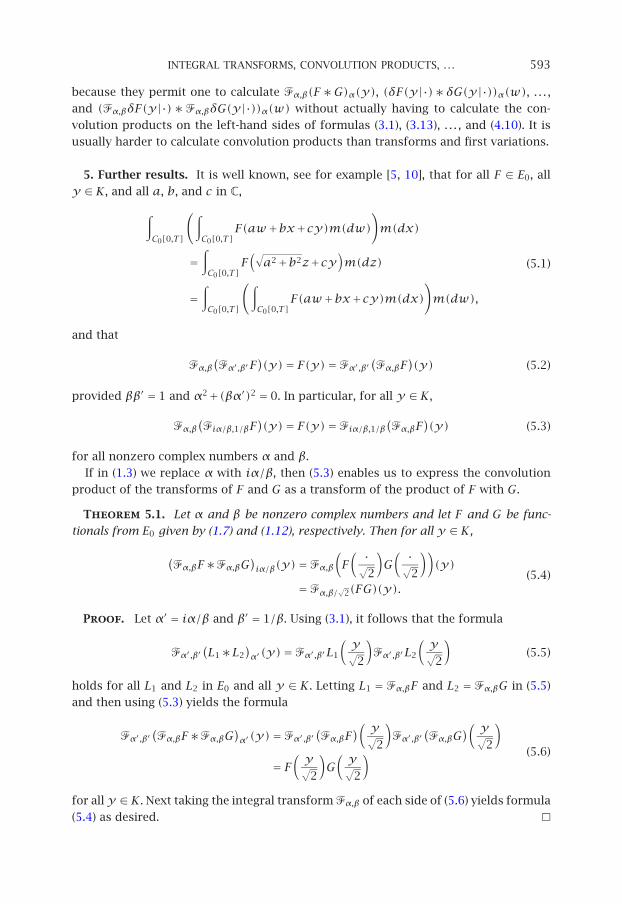
INTEGRAL TRANSFORMS, CONVOLUTION PRODUCTS, . . . 593
because they permit one to calculate �α,β(F ∗G)α(y), (δF(y|·)∗δG(y|·))α(w), . . . ,and (�α,βδF(y|·)∗�α,βδG(y|·))α(w) without actually having to calculate the con-
volution products on the left-hand sides of formulas (3.1), (3.13), . . . , and (4.10). It is
usually harder to calculate convolution products than transforms and first variations.
5. Further results. It is well known, see for example [5, 10], that for all F ∈ E0, all
y ∈K, and all a, b, and c in C,
∫C0[0,T ]
(∫C0[0,T ]
F(aw+bx+cy)m(dw))m(dx)
=∫C0[0,T ]
F(√a2+b2z+cy
)m(dz)
=∫C0[0,T ]
(∫C0[0,T ]
F(aw+bx+cy)m(dx))m(dw),
(5.1)
and that
�α,β(�α′,β′F
)(y)= F(y)=�α′,β′
(�α,βF
)(y) (5.2)
provided ββ′ = 1 and α2+(βα′)2 = 0. In particular, for all y ∈K,
�α,β(�iα/β,1/βF
)(y)= F(y)=�iα/β,1/β
(�α,βF
)(y) (5.3)
for all nonzero complex numbers α and β.
If in (1.3) we replace α with iα/β, then (5.3) enables us to express the convolution
product of the transforms of F and G as a transform of the product of F with G.
Theorem 5.1. Let α and β be nonzero complex numbers and let F and G be func-
tionals from E0 given by (1.7) and (1.12), respectively. Then for all y ∈K,
(�α,βF∗�α,βG
)iα/β(y)=�α,β
(F( ·√
2
)G( ·√
2
))(y)
=�α,β/√
2(FG)(y).(5.4)
Proof. Let α′ = iα/β and β′ = 1/β. Using (3.1), it follows that the formula
�α′,β′(L1∗L2
)α′(y)=�α′,β′L1
(y√2
)�α′,β′L2
(y√2
)(5.5)
holds for all L1 and L2 in E0 and all y ∈ K. Letting L1 = �α,βF and L2 = �α,βG in (5.5)
and then using (5.3) yields the formula
�α′,β′(�α,βF∗�α,βG
)α′(y)=�α′,β′
(�α,βF
)( y√2
)�α′,β′
(�α,βG
)( y√2
)
= F(y√2
)G(y√2
) (5.6)
for all y ∈K. Next taking the integral transform �α,β of each side of (5.6) yields formula
(5.4) as desired.

594 BONG JIN KIM ET AL.
Theorem 5.2. Let α, β, F , and G be as in Theorem 5.1. Then for all y and w in K,
δ(�α,βF∗�α,βG
)iα/β(y|w)=
β√2
�α,β(δF(·|w)G(·)+F(·)δG(·|w))( y√
2
). (5.7)
Proof. Using (5.4) and (2.25), we see that for all y and w in K,
δ(�α,βF∗�α,βG
)iα/β(y|w)= δ�α,β
(F( ·√
2
)G( ·√
2
))(y|w)
= δ�α,β/√
2
(F(·)G(·))(y|w)
= β√2
�α,β(δF(·|w)G(·)+F(·)δG(·|w))( y√
2
).
(5.8)
Next, using (5.4), we obtain the following analogue of Formula 4.8.
Theorem 5.3. Let F , G, α, and β be as in Theorem 5.1. Then for all y and w in K,
(δ�α,βF(·|w)∗δ�α,βG(·|w)
)iα/β(y)
= β2n∑l=1
n∑j=1
⟨θj,w
⟩⟨θl,w
⟩�α,β/
√2
(FjGl
)(y).
(5.9)
Proof. Using (3.4), (5.4), Theorem 2.3, and (2.23), we obtain
(δ�α,βF(·|w)∗δ�α,βG(·|w)
)iα/β(y)
= β2(�α,βδF(·|w)∗�α,βδG(·|w))iα/β(y)
= β2�α,β
(δF( ·√
2
∣∣∣∣w)δG
( ·√2
∣∣∣∣w))(y)
= β2�α,β
n∑j=1
⟨θj,w
⟩Fj( ·√
2
) n∑l=1
⟨θl,w
⟩Gl( ·√
2
)(y)
= β2n∑l=1
n∑j=1
⟨θj,w
⟩⟨θl,w
⟩�α,β/
√2
(FjGl
)(y)
(5.10)
for all y and w in K.
It is interesting to note that we can obtain analogues of Formulas 4.9 and 4.10 directly
by use of (3.13) and (3.7) rather than using Theorem 5.1 as we did in Theorem 5.3 to
obtain an analogue of Formula 4.8.
Theorem 5.4. Let F , G, α, and β be as in Theorem 5.1. Then for all y and w in K,
(δ�α,βF(y|·)∗δ�α,βG(y|·)
)iα/β(w)
= 12δ�α,βF(y|w)δ�α,βG(y|w)+ α
2
2
n∑j=1
�α,βFj(y)�α,βGj(y),
(�α,βδF(y|·)∗�α,βδG(y|·)
)iα/β(w)
= β2
2δF(y|w)δG(y|w)+ α
2
2
n∑j=1
Fj(y)Gj(y).
(5.11)
INTEGRAL TRANSFORMS, CONVOLUTION PRODUCTS, . . . 595
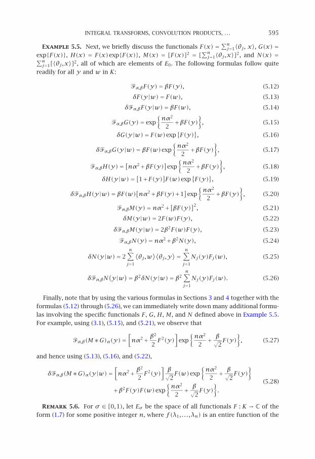
Example 5.5. Next, we briefly discuss the functionals F(x) =∑nj=1〈θj , x〉, G(x) =
exp{F(x)}, H(x) = F(x)exp{F(x)}, M(x) = [F(x)]2 = [∑nj=1〈θj,x〉]2, and N(x) =∑n
j=1[〈θj,x〉]2, all of which are elements of E0. The following formulas follow quite
readily for all y and w in K:
�α,βF(y)= βF(y), (5.12)
δF(y|w)= F(w), (5.13)
δ�α,βF(y|w)= βF(w), (5.14)
�α,βG(y)= exp{nα2
2+βF(y)
}, (5.15)
δG(y|w)= F(w)exp{F(y)
}, (5.16)
δ�α,βG(y|w)= βF(w)exp{nα2
2+βF(y)
}, (5.17)
�α,βH(y)=[nα2+βF(y)]exp
{nα2
2+βF(y)
}, (5.18)
δH(y|w)= [1+F(y)]F(w)exp{F(y)
}, (5.19)
δ�α,βH(y|w)= βF(w)[nα2+βF(y)+1
]exp
{nα2
2+βF(y)
}, (5.20)
�α,βM(y)=nα2+[βF(y)]2, (5.21)
δM(y|w)= 2F(w)F(y), (5.22)
δ�α,βM(y|w)= 2β2F(w)F(y), (5.23)
�α,βN(y)=nα2+β2N(y), (5.24)
δN(y|w)= 2n∑j=1
⟨θj,w
⟩⟨θj,y
⟩= n∑j=1
Nj(y)Fj(w), (5.25)
δ�α,βN(y|w)= β2δN(y|w)= β2
n∑j=1
Nj(y)Fj(w). (5.26)
Finally, note that by using the various formulas in Sections 3 and 4 together with the
formulas (5.12) through (5.26), we can immediately write down many additional formu-
las involving the specific functionals F , G, H, M , and N defined above in Example 5.5.
For example, using (3.1), (5.15), and (5.21), we observe that
�α,β(M∗G)α(y)=[nα2+ β
2
2F2(y)
]exp
{nα2
2+ β√
2F(y)
}, (5.27)
and hence using (5.13), (5.16), and (5.22),
δ�α,β(M∗G)α(y|w)=[nα2+ β
2
2F2(y)
]β√2F(w)exp
{nα2
2+ β√
2F(y)
}
+β2F(y)F(w)exp{nα2
2+ β√
2F(y)
}.
(5.28)
Remark 5.6. For σ ∈ [0,1), let Eσ be the space of all functionals F : K → C of the
form (1.7) for some positive integer n, where f(λ1, . . . ,λn) is an entire function of the
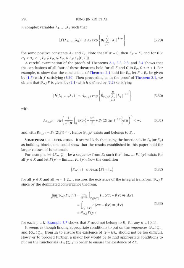
596 BONG JIN KIM ET AL.
n complex variables λ1, . . . ,λn such that
∣∣f (λ1, . . . ,λn)∣∣≤AF exp
BF
n∑j=1
∣∣λj∣∣1+σ (5.29)
for some positive constants AF and BF . Note that if σ = 0, then Eσ = E0 and for 0 <σ1 <σ2 < 1, E0 � Eσ1 � Eσ2 � L2(C0[0,T ]).
A careful examination of the proofs of Theorems 2.1, 2.2, 2.3, and 2.4 shows that
the conclusions of all four of these theorems hold for all F and G in Eσ , 0≤ σ < 1. For
example, to show that the conclusions of Theorem 2.1 hold for Eσ , let F ∈ Eσ be given
by (1.7) with f satisfying (5.29). Then proceeding as in the proof of Theorem 2.1, we
obtain that �α,βF is given by (2.1) with h defined by (2.2) satisfying
∣∣h(λ1, . . . ,λn)∣∣≤A�α,βF exp
B�α,βF
n∑j=1
∣∣λj∣∣1+σ (5.30)
with
A�α,βF =AF(
1√2π
∫R
exp{− u
2
2+BF
(2|αµ|)1+σ
}du
)n<∞, (5.31)
and with B�α,βF = BF(2|β|)1+σ . Hence �α,βF exists and belongs to Eσ .
Some possible extensions. It seems likely that using the functionals in E0 (or Eσ )
as building blocks, one could show that the results established in this paper hold for
larger classes of functionals.
For example, let {Fm}∞m=1 be a sequence from E0 such that limm→∞Fm(y) exists for
all y ∈K and let F(y)= limm→∞Fm(y). Now the condition
∣∣Fm(y)∣∣≤Aexp{B‖y‖∞
}(5.32)
for all y ∈ K and all m= 1,2, . . . ensures the existence of the integral transform �α,βFsince by the dominated convergence theorem,
limm→∞�α,βFm(y)= lim
m→∞
∫C0[0,T ]
Fm(αx+βy)m(dx)
=∫C0[0,T ]
F(αx+βy)m(dx)=�α,βF(y)
(5.33)
for each y ∈K. Example 5.7 shows that F need not belong to Eσ for any σ ∈ [0,1).It seems as though finding appropriate conditions to put on the sequences {Fm}∞m=1
and {Gm}∞m=1 from E0 to ensure the existence of (F ∗G)α should not be too difficult.
However to proceed further, a major key would be to find appropriate conditions to
put on the functionals {Fm}∞m=1 in order to ensure the existence of δF .
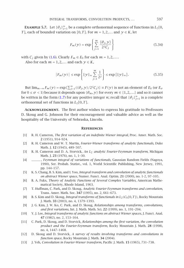
INTEGRAL TRANSFORMS, CONVOLUTION PRODUCTS, . . . 597
Example 5.7. Let {θj}∞j=1 be a complete orthonormal sequence of functions in L2[0,T ], each of bounded variation on [0,T ]. For m= 1,2, . . . and y ∈K, let
Fm(y)= exp
m∑j=1
⟨θj,y
⟩2jCj
(5.34)
with Cj given by (1.6). Clearly Fm ∈ E0 for each m= 1,2, . . . .Also for each m= 1,2, . . . and each y ∈K,
∣∣Fm(y)∣∣≤ exp
‖y‖∞
m∑j=1
12j
≤ exp
{‖y‖∞}. (5.35)
But limm→∞Fm(y)= exp{∑∞j=1(〈θj,y〉/2jCj)} ≡ F(y) is not an element of E0 (or Eσ
for 0≤ σ < 1) because it depends upon 〈θm,y〉 for everym∈ {1,2, . . .} and so it cannot
be written in the form (1.7) for any positive integer n; recall that {θj}∞j=1 is a complete
orthonormal set of functions in L2[0,T ].
Acknowledgment. The first author wishes to express his gratitude to Professors
D. Skoug and G. Johnson for their encouragement and valuable advice as well as the
hospitality of the University of Nebraska, Lincoln.
References
[1] R. H. Cameron, The first variation of an indefinite Wiener integral, Proc. Amer. Math. Soc.2 (1951), 914–924.
[2] R. H. Cameron and W. T. Martin, Fourier-Wiener transforms of analytic functionals, DukeMath. J. 12 (1945), 489–507.
[3] R. H. Cameron and D. A. Storvick, An L2 analytic Fourier-Feynman transform, MichiganMath. J. 23 (1976), no. 1, 1–30.
[4] , Feynman integral of variations of functionals, Gaussian Random Fields (Nagoya,1990), Ser. Probab. Statist., vol. 1, World Scientific Publishing, New Jersey, 1991,pp. 144–157.
[5] K. S. Chang, B. S. Kim, and I. Yoo, Integral transform and convolution of analytic functionalson abstract Wiener space, Numer. Funct. Anal. Optim. 21 (2000), no. 1-2, 97–105.
[6] B. A. Fuks, Theory of Analytic Functions of Several Complex Variables, American Mathe-matical Society, Rhode Island, 1963.
[7] T. Huffman, C. Park, and D. Skoug, Analytic Fourier-Feynman transforms and convolution,Trans. Amer. Math. Soc. 347 (1995), no. 2, 661–673.
[8] B. S. Kim and D. Skoug, Integral transforms of functionals in L2(C0[0,T ]), Rocky MountainJ. Math. 33 (2003), no. 4, 1379–1393.
[9] J. G. Kim, J. W. Ko, C. Park, and D. Skoug, Relationships among transforms, convolutions,and first variations, Int. J. Math. Math. Sci. 22 (1999), no. 1, 191–204.
[10] Y. J. Lee, Integral transforms of analytic functions on abstract Wiener spaces, J. Funct. Anal.47 (1982), no. 2, 153–164.
[11] C. Park, D. Skoug, and D. Storvick, Relationships among the first variation, the convolutionproduct and the Fourier-Feynman transform, Rocky Mountain J. Math. 28 (1998),no. 4, 1447–1468.
[12] D. Skoug and D. Storvick, A survey of results involving transforms and convolutions infunction space, Rocky Mountain J. Math. 34 (2004).
[13] J. Yeh, Convolution in Fourier-Wiener transform, Pacific J. Math. 15 (1965), 731–738.

598 BONG JIN KIM ET AL.
[14] I. Yoo, Convolution and the Fourier-Wiener transform on abstract Wiener space, RockyMountain J. Math. 25 (1995), no. 4, 1577–1587.
Bong Jin Kim: Department of Mathematics, Daejin University, Pocheon 487-711, KoreaE-mail address: [email protected]
Byoung Soo Kim: University College, Yonsei University, Seoul 120-749, KoreaE-mail address: [email protected]
David Skoug: Department of Mathematics, University of Nebraska-Lincoln, Lincoln, NE 68588-0323, USA
E-mail address: [email protected]
Advances in Difference Equations
Special Issue on
Boundary Value Problems on Time Scales
Call for Papers
The study of dynamic equations on a time scale goes backto its founder Stefan Hilger (1988), and is a new area ofstill fairly theoretical exploration in mathematics. Motivatingthe subject is the notion that dynamic equations on timescales can build bridges between continuous and discretemathematics; moreover, it often revels the reasons for thediscrepancies between two theories.
In recent years, the study of dynamic equations has ledto several important applications, for example, in the studyof insect population models, neural network, heat transfer,and epidemic models. This special issue will contain newresearches and survey articles on Boundary Value Problemson Time Scales. In particular, it will focus on the followingtopics:
• Existence, uniqueness, and multiplicity of solutions• Comparison principles• Variational methods• Mathematical models• Biological and medical applications• Numerical and simulation applications
Before submission authors should carefully read over thejournal’s Author Guidelines, which are located at http://www.hindawi.com/journals/ade/guidelines.html. Authors shouldfollow the Advances in Difference Equations manuscriptformat described at the journal site http://www.hindawi.com/journals/ade/. Articles published in this Special Issueshall be subject to a reduced Article Processing Charge ofC200 per article. Prospective authors should submit an elec-tronic copy of their complete manuscript through the journalManuscript Tracking System at http://mts.hindawi.com/according to the following timetable:
Manuscript Due April 1, 2009
First Round of Reviews July 1, 2009
Publication Date October 1, 2009
Lead Guest Editor
Alberto Cabada, Departamento de Análise Matemática,Universidade de Santiago de Compostela, 15782 Santiago deCompostela, Spain; [email protected]
Guest Editor
Victoria Otero-Espinar, Departamento de AnáliseMatemática, Universidade de Santiago de Compostela,15782 Santiago de Compostela, Spain;[email protected]
Hindawi Publishing Corporationhttp://www.hindawi.com


![Finale 2005b - [PIANOBAR for experts.MUS]jackcannon.altervista.org/PIANOBAR_for_experts_-_DEMO.pdf · Seguono due versioni di I Got Rhythm collegate ... comunque notevoli difficoltà](https://static.fdocuments.in/doc/165x107/5a788fee7f8b9ab8768cde8d/finale-2005b-pianobar-for-jackcannonaltervistaorgpianobarforexperts-demopdfseguono.jpg)


![Modifiche al testo/Amendments to the text Modifiche al testo › trasparenza › sites › default... · SSD BIO/09 (FISIOLOGIA) ... formato PDF): […] -dichiarazione di valore,](https://static.fdocuments.in/doc/165x107/5f194f33699a745cdc2db853/modifiche-al-testoamendments-to-the-text-modifiche-al-testo-a-trasparenza-a.jpg)