5 Classical Molecular Dynamics (MD) Simulations withTinker

In this set of exercises, you will be brie�y introduced to the concept of classical force�elds and molecular dynamics via propagation of atomic positions in time. You will learnhow to create molecules (methylcyclohexane) using the MOLDEN chemical editing programand you will minimise, solvate and �nally run molecular dynamics simulations on thesestructures to obtain separate trajectories for each.

5.1 Classical Molecular Dynamics

The extensive computational demand of electronic structure elucidation implies thatan exact (fully quantum mechanical) description and time-propagation of even mod-estly sized molecular systems is in practice impossible. Although systems that compriseabout 103 atoms are nowadays routinely described using approximate quantum mechan-ical (such as state-of-the-art Kohn-Sham Density Functional Theory) or semi-empiricalmethods, the computational demand of explicitly treating electrons in even larger systemssuch as biomolecules (105 atoms and more) becomes untractable all too quickly.Fortunately, for such systems it is frequently su�cient to use a classical approximation

to accurately reproduce supramolecular properties, such as the folding of a protein or thestructure of a liquid. Classical approximations typically scale better with system size,and they therefore allow both for large systems and long simulation times to be takeninto account. Here, atoms are treated as e�ective point charges with mass, instead ofnuclei with explicit electrons. The classical approach makes use of a parameterised force�eld (or classical potential energy function), which is an approximation of the quantum-mechanical potential energy surface due to the electronic and nuclear potential, as afunction of nuclear position. Such classical force �elds typically work well under thefollowing assumptions:

a) The Born-Oppenheimer approximation is valid.

b) The electronic structure is not of interest.

c) The temperature is modest.

d) There is no bond breaking or forming.

e) Electrons are highly localised.

5.1.1 Classical Approximation: Basic Features

In the classical approximation, one describes positions and momenta of all the atomicnuclei:

rN = {x1, y1, z1, . . . , xN , yN , zN} (1)

pN = {px1, py1, pz1, . . . , pxN , pyN , pzN}, (2)

1

where each position and all momenta are known simultaneously. One microstate is thencharacterised by a set of the 3N positions {rN} and 3N momenta {pN} for a total of 6Ndegrees of freedom, such that the notation {pN

m, rNm} de�nes a particular microstate m.

For any microstate, one can calculate the total energy as a sum of the kinetic T ({pN})and potential V ({rN}) terms. The Hamiltonian of a classical system then becomes:

H({pN}, {rN}) = T({pN}) + V({rN}), (3)

where the kinetic term is simply:

T({pN}) =N∑i

|pi|2

2mi. (4)

Interactions between atoms are then described by a potential energy function V({rN})that depends solely on the positions of all atoms {rN}. A key part of describing timeevolution of a molecular system classically is then the de�nition of the potential energyfunction V({rN}). In fact, the functional form of V({rN}) is often chosen by examiningthe various modes by which atoms interact according to a quantum mechanical treatmentof the molecular system and patching simple, often �rst-order theoretical expressions forthese modes together. These modes can also be �tted to experimental (and/or quantummechanical calculations of) model compounds such that the force �eld reproduces selectedproperties of a database of representative test structures.V(rN ) can be mainly decomposed into the following components:

V({rN}) = Vbonded({rN}) + Vnon−bonded({rN}), (5)

where Vbonded({rN}) and Vnon−bonded({rN}) correspond to intermolecular and in-tramolecular potentials respectively. Intramolecular interactions typically include bondstretching, bond angle bending and bond torsional modes, while intermolecular interac-tions include dispersion and coulombic potentials. These are discussed in more detailbelow.

5.1.2 Intramolecular Interactions

Intramolecular interactions occur through bonds between atoms, the three most wellknown being bond stretching (vibration), bond angle bending and bond torsional modes.These are illustrated in Figure 1.

Figure 1: Depiction of the 2, 3, and 4-centre intramolecular forces.

2

Bond Stretching An accurate description of bond stretching that well-describes theintramolecular behaviour is the empirical Morse potential:

VB(d) = De[1− e−a(d−d0)]2, (6)

where d is the length of the bond, a is a constant, d0 is the equilibrium bond length,and De is the well-depth minimum. Typically this form is not used, as it requires threeparameters per bond and is somewhat expensive to compute in simulation due to theexponential. Since the energy scales of bond stretching are relatively high, bonds rarelydeviate signi�cantly from the equilibrium bond length, thus one can use a second-orderTaylor expansion around the energy minimum:

VB(d) = α(d− d0)2, (7)

where α is a constant. This form treats bond vibrations as harmonic oscillations,and thus atoms cannot be dissociated. Figure 2 provides a depiction of both the Morsepotential and the corresponding harmonic approximation.

Figure 2: Depiction of a Morse and harmonic potential used to approximate chemicalbonds.

Bond Angle Bending This term accounts for deviations from the preferred hybridis-ation geometry (e.g sp3). Again, a common form is the second-order Taylor expansionabout the energy minimum:

VA(θ) = b(θ − θ0)2, (8)

where θ is the bond angle between three atoms, b is a constant and θ0 is the equilibriumbond angle.

3

Bond Torsions These interactions occur among four atoms and account for rotationalenergies along bonds. Unlike the previous terms, torsional modes are "soft" such thatenergies are often not so high as to only allow small deviations from an equilibriumstructure. Torsional modes are frequently modeled with the following expression:

VT (ω) =

N∑n=0

cn[1 + cos(nω − γ)], (9)

where ω is the torsional angle, n and cn are summation index and coe�cients respec-tively, and γ is an additional dihedral-dependent parameter. A depiction of VT (ω) isprovided in Figure 3.

Figure 3: A typical dihedral potential used in classical force �elds.

5.1.3 Intermolecular Interactions

Intermolecular interactions apply to any atoms that are not bonded, either within thesame molecule or between di�erent molecules.These interactions are described using a pairwise decomposition of the energy. For-

mally one can decompose the potential energy function into interactions involving singleatoms, pairs of atoms, triplets of atoms and so forth:

V({rN}) =

N∑i=1

v1(ri) +∑i=1

∑j=i+1

v2(rij) +∑i=1

∑j=i+1

∑k=j+1

v3(rij , rik, rjk) + . . . . (10)

4

It is convenient to truncate this expansion beyond pairwise interactions as the compu-tational expense of adding additional terms scales as O(Nk), where k is the number ofbodies interacting. This truncation is performed at the expense of certain polarizatione�ects which can lead to subtle deviations away from experimental results. The resultinge�ective pair potential is given by:

V({rN}) =

N∑i=1

v1(ri) +∑i=1

∑j=i+1

veff (rij). (11)

Electrostatics Interactions between charges (partial or formal) are modeled using Coulomb'slaw:

Vc(rij) =qiqj

4πε0rij, (12)

for which the atoms i and j are separated by distance rij . The partial charges aregiven by qi and qj while ε0 denotes the free space permittivity.

London Dispersion Forces Correlations between instantaneous electron densities sur-rounding two atoms gives rise to an attractive potential:

Vld(rij) ∝ r−6ij , (13)

and is a component of the Van der Waals force, which contains other forces includingdipole-dipole (Keesom force), permanent dipole-induced dipole (Debye force) and Londondispersion forces. A depiction of London dispersion and Coulombic forces can be seen inFigure 4.

Figure 4: Depiction of London dispersion and Coulombic forces.

Excluded Volume Repulsion When two atoms approach and their electron densitiesoverlap, they experience a steep increase in energy and a corresponding strong repulsion.This occurs due to the Pauli principle: two electrons are forbidden to have the same quan-tum number. At moderate inter-nuclear distances, this potential has the approximateform:

Vevr(rij) ∝ e−crij , (14)

5

where c is a constant. To alleviate computational complexity this can be successfullymodeled by a simple power law that is much more convenient to compute:

Vevr(rij) ∝ r−mij , (15)

where m is greater than 6.

Lennard-Jones Potential An e�ective method to model both the excluded volume andLondon dispersion forces is to combine them into a single expression, which Lennard-Jones proposed in the following pairwise interaction:

V(rij) = 4εij

[(rijσ

)−12−(rijσ

)−6]

(16)

where ε and σ are atom-dependent constants. The factor of 12 is used for the repulsiveterm simply because it is convenient to square the attractive r−6

ij term.

5.2 The Atomic Force Field

A bare-minimum force �eld can now be constructed as a simple addition of individualcontributions to the approximation of the potential energy surface:

V({rN}) =∑

bonds,i

αi(di−di,0)2+∑

angles,j

βj(θj−θj,0)2+∑

torsions,k

[∑n

ck,n(1 + cos(ωkn+ γk))

]

+∑i

∑j<i

qiqj4πε0rij

+ 4εij

[(rijσij

)−12

−(rijσij

)−6]. (17)

5.2.1 Force Field Parameterisation and Transferability

The minimal force �eld in section 5.2 contains a large number of parameters:

αi, di,0, βj , θj,0, ck,n, γk, qi,j , εij , σij ,

which must be chosen, depending on the kind of atoms involved and their chemical envi-ronment (e.g an oxygen-bound carbon behaves di�erently to a nitrogen-bound carbon),for every single type of bond, angle, torsion, partial charge and repulsive/dispersive inter-action. In fact, all modern force �elds typically contain more functions than the minimaland hence this results in a huge set of adjustable parameters that de�ne a particular force�eld. Classical force �elds are an area of active research, and are continually and rigor-ously developed and improved by a number of di�erent research groups. Values for theseparameters are typically taken from a combination of electronic structure calculationsof small model molecules, and also experimental data. The inclusion of experimentaldata tends to improve accuracy because it �ts bulk phases rather than the very smallsystems ab initio simulations can treat and as a result, the majority of force �elds aresemi-empirical.

6

5.3 Time Evolution

Given the potential for atomic interaction in section 5.2, the force acting upon the ithatom is determined by the gradient with respect to atomic displacements:

Fi = −∇riV (r1, . . . , rN) = −(∂V

∂xi,∂V

∂yi,∂V

∂zi

). (18)

Using Newton's equations of motion one can then achieve propagation of atomic posi-tions in time, using some time step ∆t:

ai(ri, t) =Fi(r)

mi, (19)

vi(t+ ∆t) = vi(t) + ai(t)∆t, (20)

ri(t+ ∆t) = ri(t) + vi(t)∆t. (21)

5.3.1 The Position-Verlet Algorithm

The potential energy U (r1, . . . , rN) is a function of the positions (3N) of all atoms in thesystem. Due to the complicated nature of this function and the large number of atomstypically modeled in classical systems, there is no analytical solution to the equationsof motion, and hence these must be solved numerically. The most common numericalsolutions to integrating the equations of motion are called �nite di�erence methods.First, the positions, velocities and accelerations can be approximated by a Taylor seriesexpansion:

r(t+ ∆t) = r(t) + v(t)∆t+1

2a(t)∆t2 + . . . , (22)

v(t+ ∆t) = v(t) + a(t)∆t+1

2b(t)∆t2 + . . . , (23)

a(t+ ∆t) = a(t) + b(t)∆t+ . . . , (24)

where . . . denotes higher order derivatives of r(t). One can then propagate the positionfunction forwards and backwards in time, yielding:

r(t+ ∆t) = r(t) + v(t)∆t+1

2a(t)∆t2, (25)

r(t−∆t) = r(t)− v(t)∆t+1

2a(t)∆t2, (26)

(27)

and by summing these the position-Verlet is obtained:

r(t+ ∆t) = 2r(t)− r(t−∆t) + a(t)∆t2, (28)

while the subtraction of the Taylor series for r(t+ ∆t) and r(t−∆t) yields:

v(t) =r(t+ ∆t)− r(t−∆t)

2∆t. (29)

7

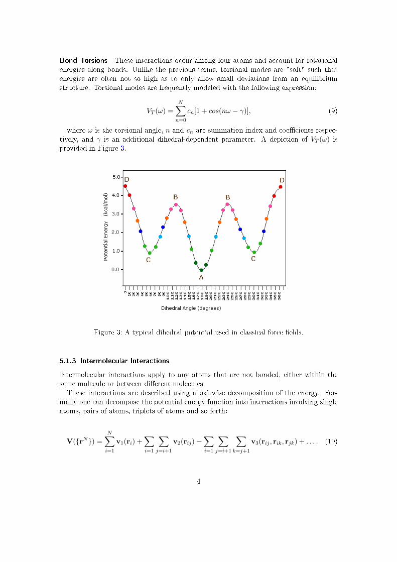
5.3.2 The Velocity-Verlet Algorithm

The position-Verlet algorithm uses positions and accelerations at time t, and the positionsfrom time t−∆t to calculate new positions at time t+∆t. The position-Verlet algorithmdoes not use velocities explicitly, and as such it is straightforward to implement andrequires minimal storage space. However, this form of the Verlet algorithm is not self-starting, i.e it requires two time steps before propagation can take place, and as suchis heavily dependent on initial starting conditions. A modi�cation to the above is thevelocity-Verlet:

r(t+ ∆t) = r(t) + v(t)∆t+1

2a(t)∆t2, (30)

v(t+ ∆t) = v(t) +1

2(a(t+ ∆t) + a(t)) ∆t, (31)

which is self-starting and additionally minimises round-o� errors.

8

5.4 Conformers in Solution: axial-methylcycohexane andequatorial-methylcyclohexane

Despite the emergence of large chemical information resources such as PubChem, �nd-ing molecular structures that are suitable starting points for computational modelingcan be a challenge. Therefore, in this exercise session you will learn the basics of howto obtain a simple classical molecular dynamics trajectory from scratch using Tinker:building molecules, de�ning force �elds, minimisation, solvation and �nally productionMD. You will begin by creating two structures in .xyz format of axial-methylcycohexaneand equatorial-methylcyclohexane respectively, shown in Figure 5. The following guideprovides a tutorial for axial-methylcyclohexane only.

H

H

H

HHH

HH

HH H H

H

H

H

HHH

H

H

Figure 5: Structures of axial-methylcyclohexane and equatorial-methylcyclohexane.These conformers of methylcyclohexane are stable in solution due to the non-negligible energetic barriers of ring �ipping at ambient temperatures.

5.4.1 Building the Structures with MOLDEN

There are a multitude 3D molecular structure builders available, but for these exercises wewill use MOLDEN. This tool provides the ability to read and write molecular structuresfrom various �le formats. Type the following to open MOLDEN:

/Applications/molden/molden4.8.command

and click on ZMAT Editor (it is advisable to do this in the Ball & Stick drawingmode).

5.4.2 ZMAT Editor: Building methylcyclohexane

Building H2 Click on Add Line in the ZMAT Editor, select hydrogen and then clicksomewhere in your MOLDEN window. You will see a single hydrogen atom appear. Next,repeat the process and instead of clicking within the MOLDEN window, click on the �rsthydrogen to create a H2 molecule. This will be your starting point for building methyl-cyclohexane.

Building axial-methylcyclohexane You will substitute the �rst hydrogen to produceyour desired structure. This is necessary since you will take a shortcut to create cyclo-hexane. Click on the �rst hydrogen (1st atom in the ZMAT Editor), click on Substitute

atom by Fragment and select CycloHexane. This will substitute your H2 molecule with

9

cyclohexane, however the dihedral of the now substituted hydrogen will be incorrect.You will need to modify the dihedral of this hydrogen (4th atom in the ZMAT Editor)from its current value to 120. Once you have done this the MOLDEN window will show acyclohexane molecule, from which you may create the conformers of methylcyclohexane.Click on one of the axial hydrogens such that it is marked with a red ball, and by selectingSubstitute atom by Fragment again, you can substitute this atom by a -CH3 group toproduce the axial-cyclohexane structure.

Assigning Atom Types Tinker requires that atom types are speci�ed in the .xyz �lesuch that the correct parameters for vibrational, angular, torsional and other contribu-tions to the force �eld can be properly assigned. For this you must make sure the ZMAT

Editor window is closed. Within the Molden Control panel, click on FF to modify atomattributes. Under the Force Field label, select Tinker MM3 and click OK. You can nowsave this �le as a tinker .xyz �le by selecting Write, then Tinker and choosing the �lename a-methylcyclohexane.xyz.You can now perform the same procedure to create the equatorial-methylcyclohexane

structure. You can either start from scratch by clicking New Z-mat from the ZMAT Editor

window or you can modify the structure by deleting and adding atoms with Delete Line

and Add Line respectively.

Adding and Removing Atoms You can add and remove atoms from the ZMAT Editor

by clicking Add Line and Delete Line respectively. Upon clicking Add line, you canthen specify which atom type you wish to add. If you are creating a new bond, you must�rst specify the atom you wish the new atom to be bonded to, followed by the atom itforms an angle with and �nally the atom with which it forms a dihedral. Specifying theseatoms is simply done by clicking in the appropriate order. To delete atoms, click on anatom in the MOLDEN (or in the ZMAT Editor) window and then click Delete Line. Youcan also modify bond lengths, angles and dihedrals explicitly by modifying the valueswithin the ZMAT Editor. If you wish to delete a Z-matrix and start over, simply clickNew Z-mat.

5.4.3 Minimisation: Specifying the Force Field

Before you begin any form of calculation with Tinker, you must create a basic .key

�le which Tinker will use to obtain system and simulation speci�c information. For thisexercise you only need to specify that you wish to use the MM3 force �eld. In yourterminal type the following command:

echo "parameters /Applications/Tinker/params/mm3.prm" > mch.key

5.4.4 Minimisation: Gas Phase

The structure created by MOLDEN is not the exact minimum energy conformer, in fact,this is impossible to guess without explicit knowledge of all bond lengths, angles and

10

dihedrals. To perturb the molecular structure to its nearest minimum, we can use theminimize program within Tinker as follows:

/Applications/Tinker/bin/minimize molecule.xyz -k molecule.key 0.01

which will minimise the structure with the MM3 force �eld supplied in the molecule.key�le, using a root mean squared (RMS) value of 0.01 as the stopping criteria for the con-vergence test. This command will produce a �le called molecule.xyz_2, which you canrename appropriately with the command:

mv molecule.xyz_2 min_molecule.xyz.

5.4.5 Energy Decomposition

You can use the Tinker program Analyze to analyse force �eld related properties. Hereit is interesting to analyse the individual contributions to the total energy, as well asdiscern the overall relative stability of a given molecule in its current con�guration andenvironment. You can use Analyze as follows:

/Applications/Tinker/bin/Analyze min_molecule.xyz -k molecule.key

and select option E to look at the total potential energy and the individual componentsthat contribute to it.

5.4.6 Solvation

To solvate the molecules in a water, you can use the waterbox.xyz �le from the previousexercise. You can copy this �le to your current directory as follows:

cp /Applications/Tinker/example/waterbox.xyz ./

You can soak your minimised molecule with the xyzedit program as follows:

/Applications/Tinker/bin/xyzedit min_molecule.xyz -k molecule.key

and choosing option #18 to add the contents of waterbox.xyz to surround yourmolecule. This will produce a solvated system called min_molecule.xyz_2 which you canrename to something more meaningful with the following command: mv min_molecule.xyz_2

solv_molecule.xyz.Since the water molecules for the previous exercise did not use the MM3 force �eld,

you will need to modify their atom types accordingly. This can be performed by loadingthe solv_molecule.xyz �le into MOLDEN and selecting the correct force �eld as before.Save this �le to something appropriate, e.g solv_molecule_mm3.xyz.

11

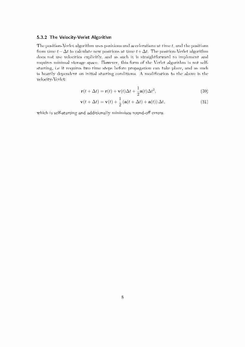
5.4.7 Molecular Dynamics

To run the simulation use the following command:

nohup /Applications/Tinker/bin/dynamic solv_molecule_mm3.xyz -k molecule.key

5000 1.0 0.1 2 298.0 &

This command speci�es that you wish to perform molecular dynamics upon the molecule.xyzsystem using parameters de�ned within the molecule.key �le. The additional parame-ters passed by command-line are:

a) Number of steps: 5000.

b) Time step length: 1.0 femtoseconds.

c) Record the output coordinates at every 0.1 picosecond.

d) Sample the canonical ensemble (Option 2).

e) Temperature held constant at 298.0K.

And �nally the output of the simulation is piped to the �le nohup.out which you cantrack the progress of by typing the following command:

tail -10 nohup.out

where the -10 �ag will make tail print the last 10 lines of the nohup.out �le to yourterminal.

5.4.8 Creating the Trajectory

The above dynamics will produce 50 snapshots of the system, saved in the �les named`solv_molecule_mm3.001...solv_molecule_mm3.050'. These �les contain the coordi-nates of the trajectory at every 0.1 picosecond. To visualise this trajectory, you must�rst compile them together into a single archive using the following program:

/Applications/Tinker/bin/archive

You will be asked to enter the name of the coordinate archive �le. Enter `solv_molecule_mm3'and then `1' to indicate that you are compressing a set of frames. you will now need toenter the frames over which the dynamics was recorded, so enter `001 050'. This willproduce a solv_molecule_mm3.arc �le which can be loaded into VMD:

/Applications/VMD/VMD\ 1.9.1.app/Contents/vmd/vmd_MACOSXX86 solv_molecule_mm3.arc

12

5.4.9 Creating the Trajectory: Modi�cations

If the solv_molecule_mm3.arc �le produced above does not load into VMD immediately,it will need a small amount of editing. Open the �le in vi as follows:

vi solv_molecule_mm3.arc

and type the following command:

:%s/ 24.662000.*\n//ge

and press enter. Note that there are 4 spaces between the �rst / and the numeral 2.This command will remove the second line (containing simulation box information) fromevery frame in the archive.

5.5 Exercises

5.5.1 Time Evolution

a) Derive the form of r(t + ∆t) in the velocity-Verlet (equation 30). Hint: solveequation 29 for r(t−∆t), and use equations 28 and 25.

b) Derive the form of v(t + ∆t) in the velocity-Verlet (equation 30). Hint: recastequations 29 and 28 to a timestep ∆t in the future, and use the result obtainedabove.

5.5.2 Conformer Preparation

Create initial starting structures for both conformers of methylcyclohexane and minimisethem in the gas phase. Use the Analyse program to investigate the main components ofthe total potential energy for the initial and minimised (gas phase) structures for bothconformers of methylcyclohexane.

a) For one of the minimised conformers, provide the entire Tinker .xyz in your reportand comment upon the main di�erences between this and a standard .xyz �le.Why are these di�erences important for using Tinker?

b) Include images of both the initial and minimised structures in your report.

c) Tabulate the potential energy components in your report, including the total energyfor both the initial and minimised structures. Which components change the mostduring the minimisation process?

d) What are the largest contributions to the potential energy, which molecule is morestable (in the gas phase) and why?

Note: You can visualise Tinker .xyz �les in VMD by loading them as new molecules,and selecting the Tinker format.

13

5.5.3 Running Classical Molecular Dynamics

Solvate the minimised molecules separately and perform molecular dynamics of bothsystems for a total duration of 50ps, with the MM3 force �eld. Using the Tinker archiveprogram, create a trajectory from the MD and visualise it in VMD.

a) Include a frame from the MD simulation within your report.

b) From one of your trajectories, tabulate the following averages in your report: theH3C-CH2-C5H9 bond length, one of the CH3-CH2-C5H9 angles and one of theH-CH2-CH2-C5H9 dihedrals. Do the averages you have computed correspond tothose in the mm3.prm �le? Why?

c) Plot the g(r) functions (using 'name O' as both selection criteria) for both solvatedconformers and include the g(r) graphs in your report. Comment upon why thesegraphs have such a signi�cant 2nd solvation shell, versus that of the pure water yousimulated in exercise 4.

Note: You can track changes in a given property (bond, angle or dihedral) with VMD.First open the Mouse menu from the VMD Main window, and select the appropriate prop-erty from the Label item. Your mouse has now changed into label mode, and from hereyou can select the appropriate atoms. Once you have selected the correct atoms, clickthe Labels... item from the Graphics menu option in the VMD Main window. SelectBonds, Angles or Dihedrals from the drop-down menu, and go to the Graph tab. Hereyou can choose to Graph... the data over the course of the trajectory, or save the dataas a .dat �le, from which you can calculate the average.

14