5-1Capacity Planning William J. Stevenson Long-Range Capacity Planning 9 th edition.

5-1 Capacity Planning

William J. Stevenson

Long-Range Capacity Planning

9th edition


5-2

Learning ObjectivesLearning Objectives

Explain the importance of capacity planning. Discuss ways of defining and measuring

capacity. Describe the determinants of effective capacity. Discuss the major considerations related to

developing capacity alternatives. Briefly describe approaches that are useful for

evaluating capacity alternatives


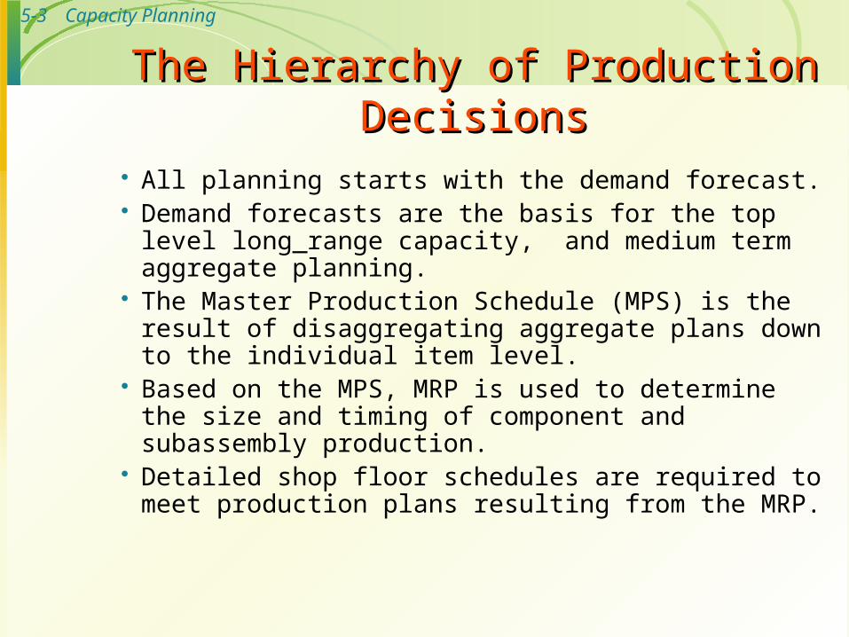
The Hierarchy of Production The Hierarchy of Production DecisionsDecisions

All planning starts with the demand forecast. Demand forecasts are the basis for the top level long_range

capacity, and medium term aggregate planning. The Master Production Schedule (MPS) is the result of

disaggregating aggregate plans down to the individual item level.

Based on the MPS, MRP is used to determine the size and timing of component and subassembly production.

Detailed shop floor schedules are required to meet production plans resulting from the MRP.

5-4 Capacity PlanningHierarchy of Hierarchy of

Production DecisionsProduction Decisions

Long-range Capacity PlanningLong-range Capacity Planning


Capacity PlanningCapacity Planning

Capacity is the upper limit or ceiling on the load that an operating unit can handle.

The basic questions in capacity handling are: What kind of capacity is needed? How much is needed? (Forecasts are key

inputs) When is it needed?


Importance of Capacity DecisionsImportance of Capacity Decisions

Capacity decisions are important to all departments of the organization;

An accountant would be interested in collecting cost accounting information in order to ensure that correct capacity expansion decision is reached.



Similarly a financial manager would be interested in performing the financial analysis of whether the investment decision is justified for a plant or capacity increase.



An Information Technology Manager would end up preparing data bases that would aid the organization to decide about the capacity and last but not the least an operations manager would select strategies that would help the organization achieve the optimum capacity levels to meet the customer demand.


1. Impacts ability to meet future demands2. Affects operating costs3. Major determinant of initial costs4. Involves long-term commitment5. Affects competitiveness6. Affects ease of management7. Globalization adds complexity8. Impacts long range planning


5-10 Capacity PlanningGlobalization adds complexityGlobalization adds complexity

Capacity decision often involves making a decision in a foreign country which requires the management to know about the political, economic and cultural issues.


CapacityCapacity

Design capacity maximum output rate or service capacity an

operation, process, or facility is designed for Effective capacity

Design capacity minus allowances such as personal time, maintenance, and scrap

Actual output rate of output actually achieved--cannot

exceed effective capacity.


Efficiency and UtilizationEfficiency and Utilization

Actual outputEfficiency =

Effective capacity

Actual outputUtilization =

Design capacity

Both measures expressed as percentages


Actual output = 36 units/day Efficiency = =

90% Effective capacity 40 units/ day

Utilization = Actual output = 36 units/day =

72% Design capacity 50 units/day

Efficiency/Utilization ExampleEfficiency/Utilization Example

Design capacity = 50 trucks/day

Effective capacity = 40 trucks/day

Actual output = 36 units/day


Key Decisions of Capacity PlanningKey Decisions of Capacity Planning

1. Amount of capacity needed

2. Timing of changes

3. Need to maintain balance

4. Extent of flexibility of facilities

Capacity cushion – extra demand intended to offset uncertaintyThe greater the degree of demand uncertainity, the greater the amount of cushion


Steps for Capacity PlanningSteps for Capacity Planning

1. Estimate future capacity requirements

2. Evaluate existing capacity

3. Identify alternatives

4. Conduct financial analysis

5. Assess key qualitative issues

6. Select one alternative

7. Implement alternative chosen

8. Monitor results


5-16

Calculating Processing Calculating Processing RequirementsRequirements

P r o d u c tA n n u a l

D e m a n d

S t a n d a r dp r o c e s s i n g t i m e

p e r u n i t ( h r . )P r o c e s s i n g t i m e

n e e d e d ( h r . )

# 1

# 2

# 3

4 0 0

3 0 0

7 0 0

5 . 0

8 . 0

2 . 0

2 , 0 0 0

2 , 4 0 0

1 , 4 0 0 5 , 8 0 0

P r o d u c tA n n u a l

D e m a n d

S t a n d a r dp r o c e s s i n g t i m e

p e r u n i t ( h r . )P r o c e s s i n g t i m e

n e e d e d ( h r . )

# 1

# 2

# 3

4 0 0

3 0 0

7 0 0

5 . 0

8 . 0

2 . 0

2 , 0 0 0

2 , 4 0 0

1 , 4 0 0 5 , 8 0 0

If annual capacity is 2000 (8hr/day*250 days *1 machine) hours, then we need three machines to handle the required volume: 5,800 hours/2,000 hours = 2.90 machines


5-17

Need to be near customers Capacity and location are closely tied

Inability to store services Capacity must be matched with timing of

demand Degree of volatility of demand

Peak demand periods

Planning Service CapacityPlanning Service Capacity


http://www.baskent.edu.tr/~kilter

18

Make or Buy? Make or Buy? Available capacity. If an organization has available the equipment, necessary skills, and time, it often

makes sense to produce an item or perform a service in-house.

Expertise. If a firm lacks the expertise to do a job satisfactorily, buying might be a reasonable alternative.

Quality considerations. Firms that specialize can usually offer higher quality than an organization can attain itself. Conversely, unique quality requirements or the desire to closely monitor quality may cause an organization to perform a job itself.

The nature of demand. When demand for an item is high and steady, the organization is often better off doing the work itself. However, wide fluctuations in demand or small orders are usually better handled by specialists who are able to combine orders from multiple sources, which results in higher volume and tends to offset individual buyer fluctuations.

Cost. Cost savings might come from the item itself or from transportation cost savings. If there are fixed costs associated with making an item that cannot be reallocated if the service or product is outsourced, that has to be recognized in the analysis. Conversely, outsourcing may help a firm avoid incurring fixed costs.

Risk. Outsourcing may involve certain risks. One is loss of control over operations. Another is the need to disclose proprietary information.


5-19

Capacity Planning Based-on Capacity Planning Based-on Bottleneck OperationBottleneck Operation

Figure 5.2

Machine #2Machine #2BottleneckOperation

BottleneckOperation

Machine #1Machine #1



10/hr

10/hr

10/hr

10/hr

30/hr

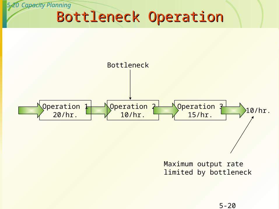
Bottleneck operation: An operationin a sequence of operations whosecapacity is lower than that of theother operations


5-20

Bottleneck OperationBottleneck Operation

Operation 120/hr.

Operation 210/hr.

Operation 315/hr.

10/hr.

Bottleneck

Maximum output ratelimited by bottleneck


Developing Capacity AlternativesDeveloping Capacity Alternatives

1. Design flexibility into systems

2. Take stage of life cycle into account

3. Take a “big picture” approach to capacity changes

4.Prepare to deal with capacity “chunks”

5. Attempt to smooth out capacity requirements

(due to random variations or seasonal variations)

6. Identify the optimal operating level


Prepare to deal with capacity “chunks.” Capacity increases are often acquired in fairly large chunks rather than smooth increments, making it difficult to achieve a match between desired capacity and feasible capacity.

Attempt to smooth out capacity requirements. Unevenness in capacity requirements also can create certain problems.

http://www.baskent.edu.tr/~kilter

22


Economies of ScaleEconomies of Scale

Economies of scale If the output rate is less than the optimal level,

increasing output rate results in decreasing average unit costs. This results from fixed costs, labor cost being spread over more units

Diseconomies of scale If the output rate is more than the optimal level,

increasing the output rate results in increasing average unit costs. Due to scheduling problems, quality problems, reduced morale, increased use of overtime.


Evaluating AlternativesEvaluating Alternatives

Minimumcost

Av

era

ge

co

st

per

un

it

0 Rate of output

Production units have an optimal rate of output for minimal cost.

Figure 5.3

Minimum average cost per unit


Economies and Diseconomies of ScaleEconomies and Diseconomies of Scale

Average UnitAverage UnitCost of Output ($)Cost of Output ($)

Annual Volume (units)Annual Volume (units)

Best Operating LevelBest Operating Level

EconomiesEconomiesof Scaleof Scale

DiseconomiesDiseconomiesof Scaleof Scale

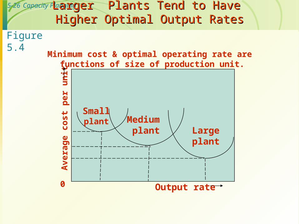
5-26 Capacity PlanningLarger Plants Tend to Have Larger Plants Tend to Have Higher Optimal Output RatesHigher Optimal Output Rates

Minimum cost & optimal operating rate are functions of size of production unit.

Av

era

ge

co

st

per

un

it

0

Smallplant Medium

plant Largeplant

Output rate

Figure 5.4


5-27

Evaluating AlternativesEvaluating Alternatives

Cost-volume analysis Break-even point

Financial analysis Cash flow Present value

Decision theory Waiting-line analysis Simulation


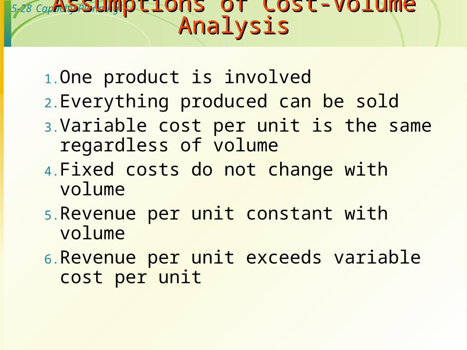
1. One product is involved2. Everything produced can be sold3. Variable cost per unit is the same regardless

of volume4. Fixed costs do not change with volume5. Revenue per unit constant with volume6. Revenue per unit exceeds variable cost per

unit

Assumptions of Cost-Volume AnalysisAssumptions of Cost-Volume Analysis


Cost-Volume RelationshipsCost-Volume Relationships

Am

ou

nt

($)

0Q (volume in units)

Total cost = VC + FC

Total variable cost (V

C)

Fixed cost (FC)

Figure 5.5a



Am

ou

nt

($)

Q (volume in units)0

Total r

evenue

Figure 5.5b



Am

ou

nt

($)

Q (volume in units)0 BEP units

Profit

Total r

even

ue

Total cost

Figure 5.5c


Break-Even Problem with Step Fixed CostsBreak-Even Problem with Step Fixed Costs

Quantity

FC + VC = TC

FC + VC = TC

FC + VC =

TC

Step fixed costs and variable costs.

1 machine

2 machines

3 machines

Figure 5.6a


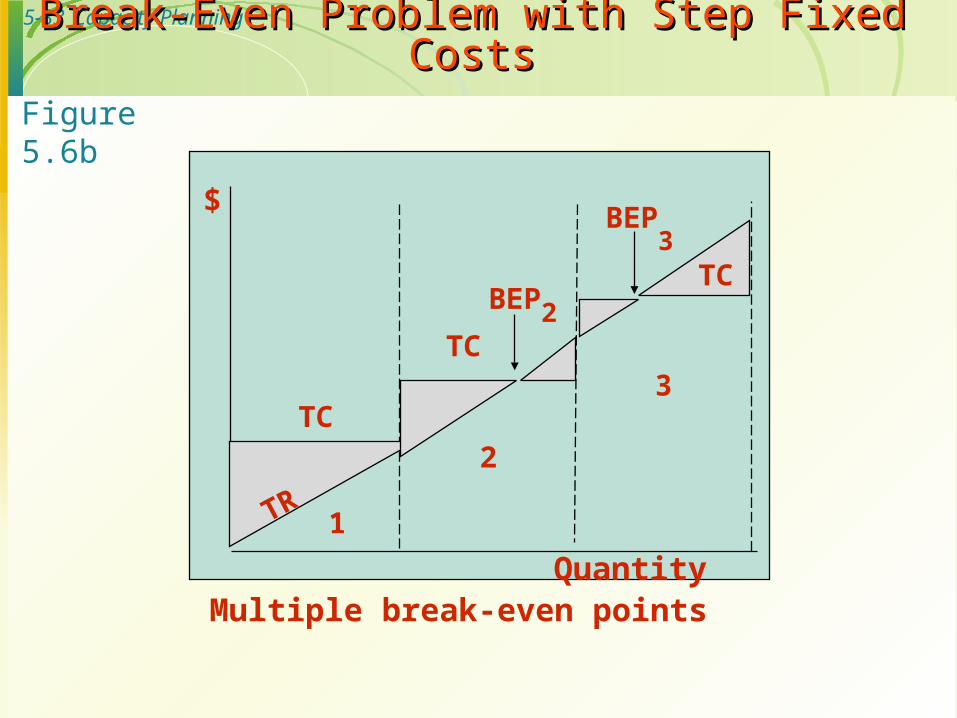
Break-Even Problem with Step Fixed CostsBreak-Even Problem with Step Fixed Costs

$

TC

TC

TCBEP2

BEP3

TR

Quantity

1

2

3

Multiple break-even points

Figure 5.6b


Example 4: page 195Example 4: page 195

A manager has the option of purchasing one, two, or three machines.

# of mach. Tot. Annual FC Correspond. Output

1 $9600 0 – 300

2 15000 301 - 600

3 20000 601 – 900

Variable cost is $10, revenue is $40 per unit.a) Determine the break-even point for each range.

b) If projected demand is between 580 and 660 units, how many machines should the manager purchase?


Example 2Example 2

a) For one machine Q = 9600/(40-10)= 320 units

For two machines Q= 15000/(40-10)= 500 units

For three machines Q=20000/(40-10)=666.67 units

b) Manager should choose two machines. Because even if demand is at low end of the range (i.e., 580), it would be above the break-even point and thus yield a profit. If three machines are purchased, even at the top end of projected demand (i.e., 660), the volume would still be less than the break-even point for that range, so there would be no profit.


Financial AnalysisFinancial Analysis

Cash Flow - the difference between cash received from sales and other sources, and cash outflow for labor, material, overhead, and taxes.

Present Value - the sum, in current value, of all future cash flows of an investment proposal.


Decision Tree AnalysisDecision Tree Analysis

Structures complex, multiphase decisions Allows objective evaluation of alternatives Incorporates uncertainty Develops expected values


Good Eats Café is about to build a new restaurant. An architect has developed three building designs, each with a different seating capacity. Good Eats estimates that the average number of customers per hour will be 80, 100, or 120 with respective probabilities of 0.4, 0.2, and 0.4. The payoff table showing the profits for the three designs is on the next slide.

Example: Decision Tree AnalysisExample: Decision Tree Analysis


Payoff Table

Average Number of Customers Per Hour

c1 = 80 c2 = 100 c3 = 120

Design A $10,000 $15,000 $14,000

Design B $ 8,000 $18,000 $12,000

Design C $ 6,000 $16,000 $21,000

Example: Decision Tree AnalysisExample: Decision Tree Analysis


Expected Value For Each DecisionExpected Value For Each Decision

Choose the design with largest EV -- Design C.Choose the design with largest EV -- Design C.

3333

4444

dd11

dd22

dd33

EV = .4(10,000) + .2(15,000) + .4(14,000)EV = .4(10,000) + .2(15,000) + .4(14,000) = $12,600= $12,600

EV = .4(8,000) + .2(18,000) + .4(12,000)EV = .4(8,000) + .2(18,000) + .4(12,000) = $11,600= $11,600

EV = .4(6,000) + .2(16,000) + .4(21,000)EV = .4(6,000) + .2(16,000) + .4(21,000) = = $14,000$14,000

Design ADesign A

Design BDesign B

Design CDesign C

2222

1 1 1 1

Example: Decision Tree AnalysisExample: Decision Tree AnalysisExample: Decision Tree AnalysisExample: Decision Tree Analysis


5-41

Waiting-Line AnalysisWaiting-Line Analysis

Useful for designing or modifying service systems Waiting-lines occur across a wide variety of

service systems Waiting-lines are caused by bottlenecks in the

process Helps managers plan capacity level that will be

cost-effective by balancing the cost of having customers wait in line with the cost of additional capacity

5-1Capacity Planning William J. Stevenson Long-Range Capacity Planning 9 th edition.

Documents

Transcript of 5-1Capacity Planning William J. Stevenson Long-Range Capacity Planning 9 th edition.