
454 Course Overview
34
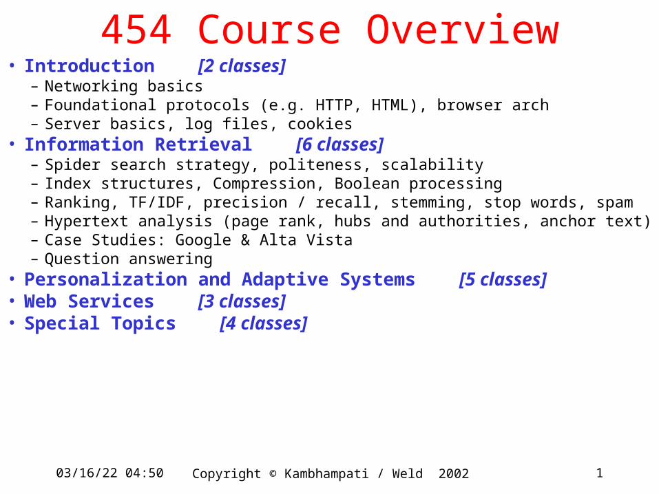
03/16/22 04:50 1 Copyright © Kambhampati / Weld 2002 454 Course Overview • Introduction [2 classes] – Networking basics – Foundational protocols (e.g. HTTP, HTML), browser arch – Server basics, log files, cookies • Information Retrieval [6 classes] – Spider search strategy, politeness, scalability – Index structures, Compression, Boolean processing – Ranking, TF/IDF, precision / recall, stemming, stop words, spam – Hypertext analysis (page rank, hubs and authorities, anchor text) – Case Studies: Google & Alta Vista – Question answering • Personalization and Adaptive Systems [5 classes] • Web Services [3 classes] • Special Topics [4 classes]
-
Upload
davis-king -
Category
Documents
-
view
24 -
download
0
description
454 Course Overview. Introduction [2 classes] Networking basics Foundational protocols (e.g. HTTP, HTML), browser arch Server basics, log files, cookies Information Retrieval [6 classes] Spider search strategy, politeness, scalability - PowerPoint PPT Presentation
Transcript of 454 Course Overview
04/19/23 21:27 1Copyright © Kambhampati / Weld 2002
454 Course Overview• Introduction [2 classes]
– Networking basics – Foundational protocols (e.g. HTTP, HTML), browser arch– Server basics, log files, cookies
• Information Retrieval [6 classes] – Spider search strategy, politeness, scalability– Index structures, Compression, Boolean processing– Ranking, TF/IDF, precision / recall, stemming, stop words, spam – Hypertext analysis (page rank, hubs and authorities, anchor text) – Case Studies: Google & Alta Vista– Question answering
• Personalization and Adaptive Systems [5 classes] • Web Services [3 classes] • Special Topics [4 classes]
04/19/23 21:27 2Copyright © Kambhampati / Weld 2002
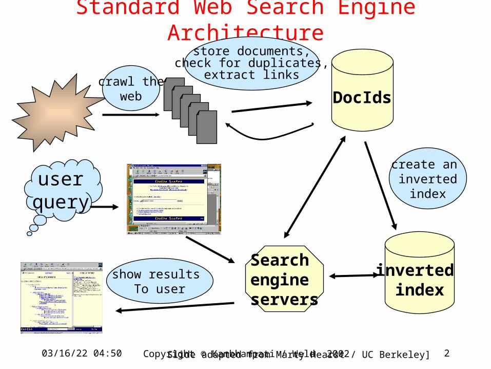
Standard Web Search Engine Architecture
crawl theweb
create an inverted
index
store documents,check for duplicates,
extract links
inverted index
DocIds
Slide adapted from Marty Hearst / UC Berkeley]
Search engine servers
userquery
show results To user

04/19/23 21:27 3Copyright © Kambhampati / Weld 2002
Review• Precision & Recall metrics• Vector Space Representation
– Dot Product as Similarity Metric
• TF-IDF for Computing Weights– wij = f(i,j) * log(N/ni)
• Relevance Feedback• Latent Semantic Indexing
– Reduce Dimensionality of Matrix– Still use Dot product
• But How Process Efficiently?
documents
term
s
q djt1
t2

04/19/23 21:27 4Copyright © Kambhampati / Weld 2002
Search Engine Components
• Spider– Getting the pages
• Indexing– Storing (e.g. in an inverted file)
• Query Processing– Booleans, …
• Ranking– Vector space model, PageRank, nnchor text analysis
• Summaries• Refinement

04/19/23 21:27 5Copyright © Kambhampati / Weld 2002
Efficient Retrieval
• Document-term matrix
t1 t2 . . . tj . . . tm nf
d1 w11 w12 . . . w1j . . . w1m 1/|d1| d2 w21 w22 . . . w2j . . . w2m 1/|d2|
. . . . . . . . . . . . . .
di wi1 wi2 . . . wij . . . wim 1/|di|
. . . . . . . . . . . . . . dn wn1 wn2 . . . wnj . . . wnm 1/|dn|
• wij is the weight of term tj in document di
• Most wij’s will be zero.
04/19/23 21:27 6Copyright © Kambhampati / Weld 2002
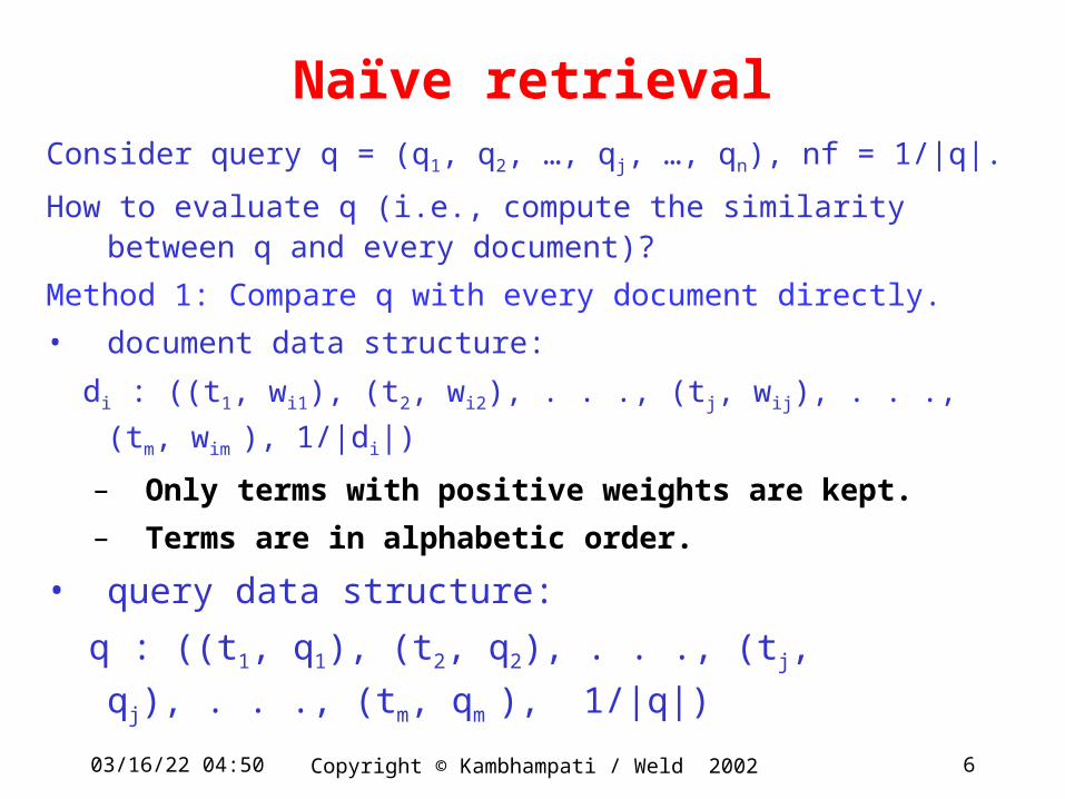
Naïve retrievalConsider query q = (q1, q2, …, qj, …, qn), nf = 1/|q|.
How to evaluate q (i.e., compute the similarity between q and every document)?
Method 1: Compare q with every document directly.
• document data structure:
di : ((t1, wi1), (t2, wi2), . . ., (tj, wij), . . ., (tm, wim ), 1/|di|)
– Only terms with positive weights are kept.
– Terms are in alphabetic order.
• query data structure:
q : ((t1, q1), (t2, q2), . . ., (tj, qj), . . ., (tm, qm ), 1/|q|)

04/19/23 21:27 7Copyright © Kambhampati / Weld 2002
Naïve retrieval
Method 1: Compare q with documents directly (cont.)
• Algorithm
initialize all sim(q, di) = 0;
for each document di (i = 1, …, n)
{ for each term tj (j = 1, …, m)
if tj appears in both q and di
sim(q, di) += qj wij;
sim(q, di) = sim(q, di) (1/|q|) (1/|di|); }
sort documents in descending similarities and
display the top k to the user;

04/19/23 21:27 8Copyright © Kambhampati / Weld 2002
Observation
• Method 1 is not efficient– Need to be access most non-zero entries in doc-term matrix.
• Solution: Inverted Index– Data structure to permit fast searching.
• Like an Index in the back of a text book.– Key words --- page numbers.– E.g, precision, 40, 55, 60-63, 89, 220– Lexicon– Occurrences

04/19/23 21:27 9Copyright © Kambhampati / Weld 2002
Search Processing (Overview)
• Lexicon search– E.g. looking in index to find entry
• Retrieval of occurrences– Seeing where term occurs
• Manipulation of occurrences– Going to the right page
04/19/23 21:27 10Copyright © Kambhampati / Weld 2002
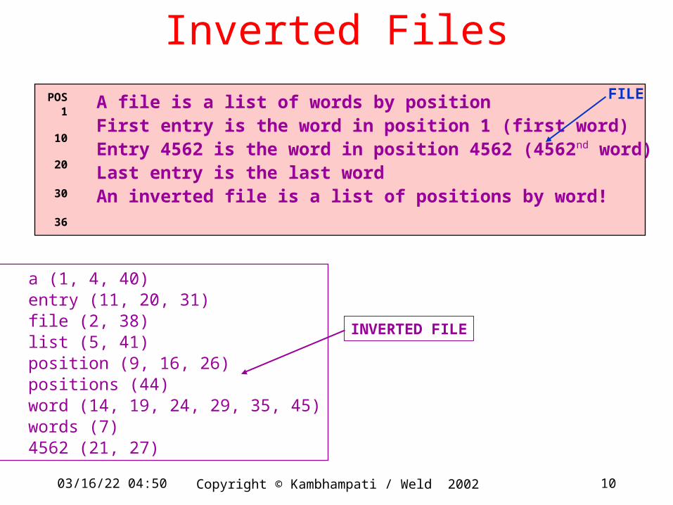
Inverted Files
A file is a list of words by positionFirst entry is the word in position 1 (first word)Entry 4562 is the word in position 4562 (4562nd word)Last entry is the last wordAn inverted file is a list of positions by word!
POS1
10
20
30
36
FILE
a (1, 4, 40)entry (11, 20, 31)file (2, 38)list (5, 41)position (9, 16, 26)positions (44)word (14, 19, 24, 29, 35, 45)words (7)4562 (21, 27)
INVERTED FILE

04/19/23 21:27 11Copyright © Kambhampati / Weld 2002
Inverted Files for Multiple Documents
107 4 322 354 381 405232 6 15 195 248 1897 1951 2192677 1 481713 3 42 312 802
WORD NDOCS PTR
jezebel 20
jezer 3
jezerit 1
jeziah 1
jeziel 1
jezliah 1
jezoar 1
jezrahliah 1
jezreel 39jezoar
34 6 1 118 2087 3922 3981 500244 3 215 2291 301056 4 5 22 134 992
DOCID OCCUR POS 1 POS 2 . . .
566 3 203 245 287
67 1 132. . .
“jezebel” occurs6 times in document 34,3 times in document 44,4 times in document 56 . . .
LEXICON
OCCURENCE INDEX
• One method. Alta Vista uses alternative

04/19/23 21:27 12Copyright © Kambhampati / Weld 2002
Many Variations Possible
• Address space (flat, hierarchical)
• Position
• TF /IDF info precalculated
• Header, font, tag info stored
• Compression strategies

04/19/23 21:27 13Copyright © Kambhampati / Weld 2002
Using Inverted Files
Several data structures:
1. For each term tj, create a list (inverted file list) that
contains all document ids that have tj.
I(tj) = { (d1, w1j), (d2, w2j), …, (di, wij), …, (dn, wnj) }
– di is the document id number of the ith document.
– Weights come from freq of term in doc
– Only entries with non-zero weights should be kept.
04/19/23 21:27 14Copyright © Kambhampati / Weld 2002
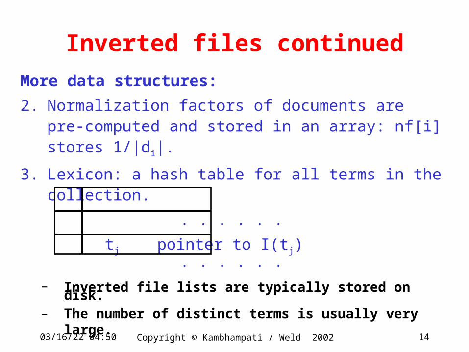
Inverted files continued
More data structures:
2. Normalization factors of documents are pre-computed and stored in an array: nf[i] stores 1/|di|.
3. Lexicon: a hash table for all terms in the collection.
. . . . . .
tj pointer to I(tj) . . . . . .
– Inverted file lists are typically stored on disk.– The number of distinct terms is usually very large.
04/19/23 21:27 15Copyright © Kambhampati / Weld 2002
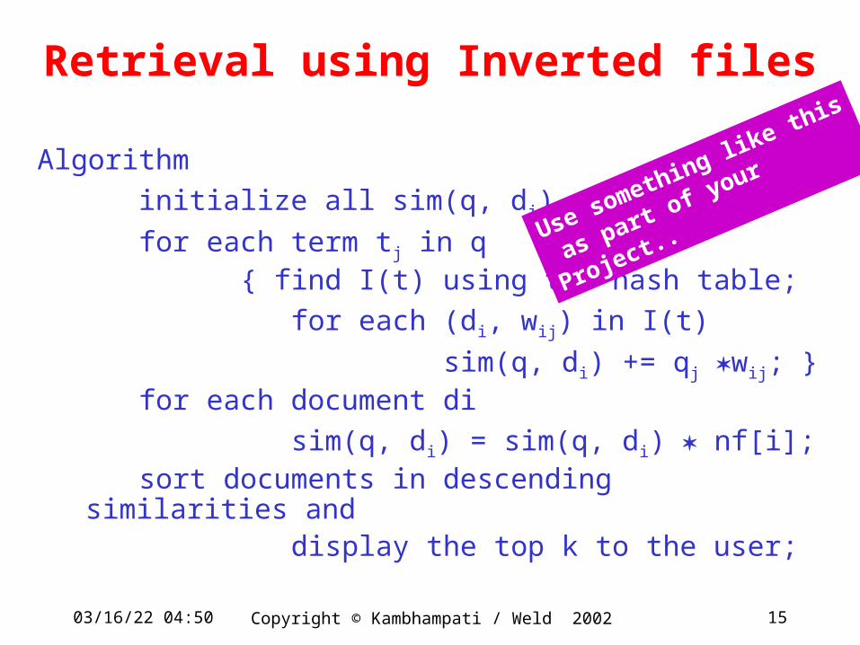
Retrieval using Inverted files
Algorithm
initialize all sim(q, di) = 0;
for each term tj in q { find I(t) using the hash table;
for each (di, wij) in I(t)
sim(q, di) += qj wij; } for each document di
sim(q, di) = sim(q, di) nf[i]; sort documents in descending similarities and display the top k to the user;
Use something like this
as part of your
Project..

04/19/23 21:27 16Copyright © Kambhampati / Weld 2002
Observations about Method 2
• If a document d does not contain any term of a given query q, then d will not be involved in the evaluation of q.
• Only non-zero entries in the columns in the document-term matrix corresponding to the query terms are used to evaluate the query.
• Computes the similarities of multiple documents simultaneously (w.r.t. each query word)
04/19/23 21:27 17Copyright © Kambhampati / Weld 2002
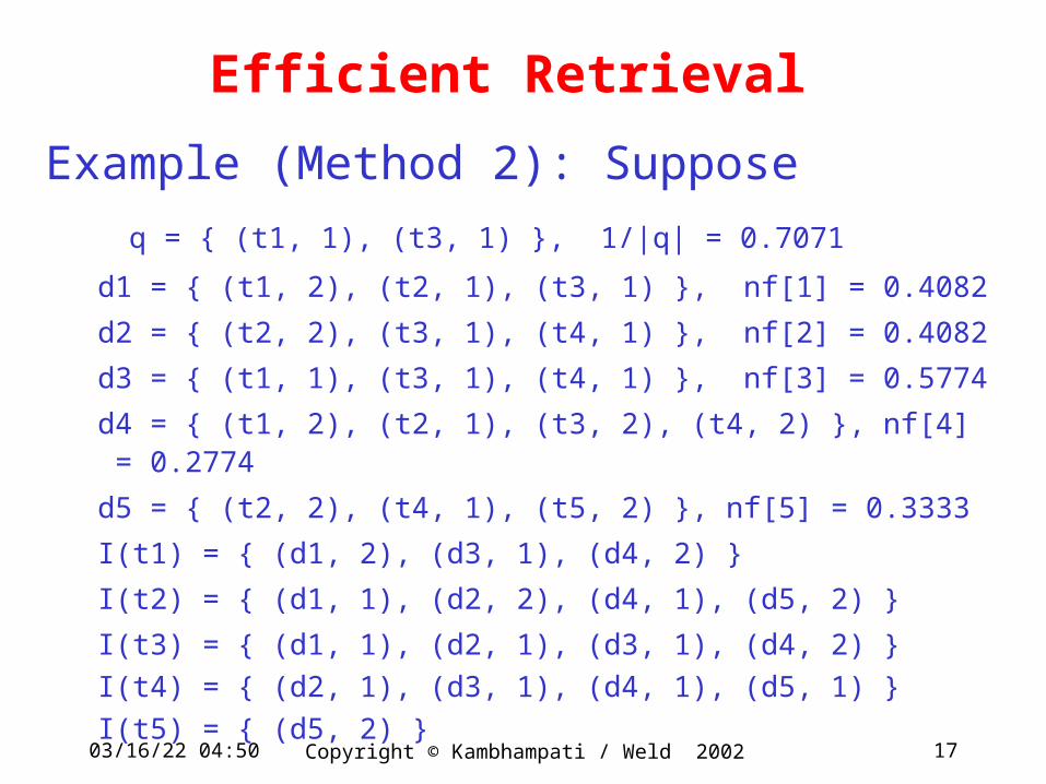
Efficient Retrieval
Example (Method 2): Suppose
q = { (t1, 1), (t3, 1) }, 1/|q| = 0.7071
d1 = { (t1, 2), (t2, 1), (t3, 1) }, nf[1] = 0.4082
d2 = { (t2, 2), (t3, 1), (t4, 1) }, nf[2] = 0.4082
d3 = { (t1, 1), (t3, 1), (t4, 1) }, nf[3] = 0.5774
d4 = { (t1, 2), (t2, 1), (t3, 2), (t4, 2) }, nf[4] = 0.2774
d5 = { (t2, 2), (t4, 1), (t5, 2) }, nf[5] = 0.3333
I(t1) = { (d1, 2), (d3, 1), (d4, 2) }
I(t2) = { (d1, 1), (d2, 2), (d4, 1), (d5, 2) }
I(t3) = { (d1, 1), (d2, 1), (d3, 1), (d4, 2) }
I(t4) = { (d2, 1), (d3, 1), (d4, 1), (d5, 1) }
I(t5) = { (d5, 2) }
04/19/23 21:27 18Copyright © Kambhampati / Weld 2002
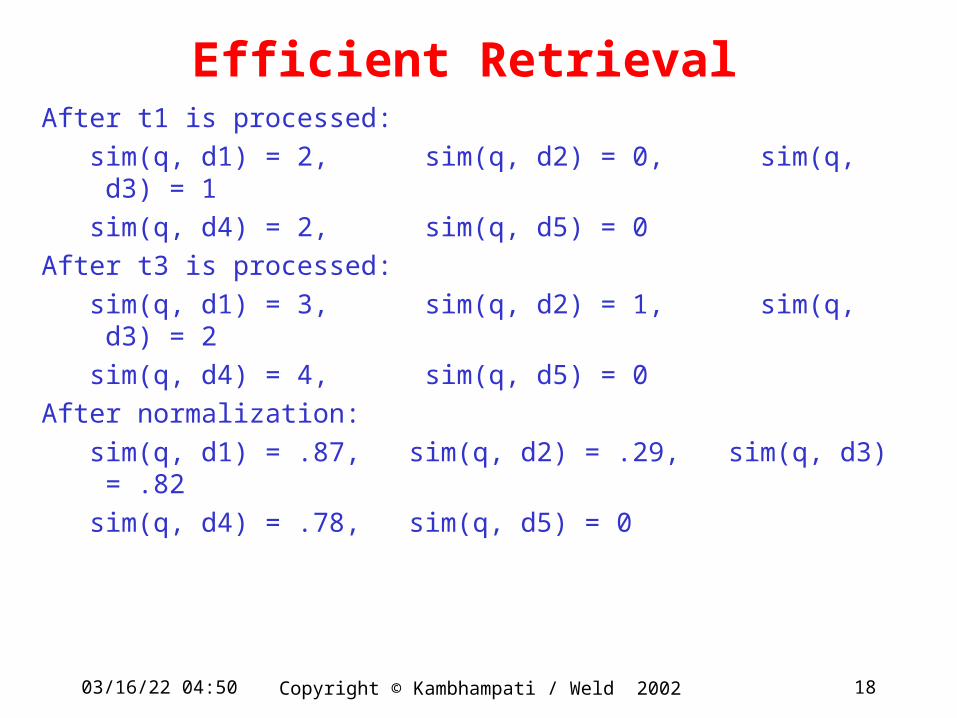
Efficient Retrieval After t1 is processed:
sim(q, d1) = 2, sim(q, d2) = 0, sim(q, d3) = 1
sim(q, d4) = 2, sim(q, d5) = 0
After t3 is processed:
sim(q, d1) = 3, sim(q, d2) = 1, sim(q, d3) = 2
sim(q, d4) = 4, sim(q, d5) = 0
After normalization:
sim(q, d1) = .87, sim(q, d2) = .29, sim(q, d3) = .82
sim(q, d4) = .78, sim(q, d5) = 0
04/19/23 21:27 19Copyright © Kambhampati / Weld 2002
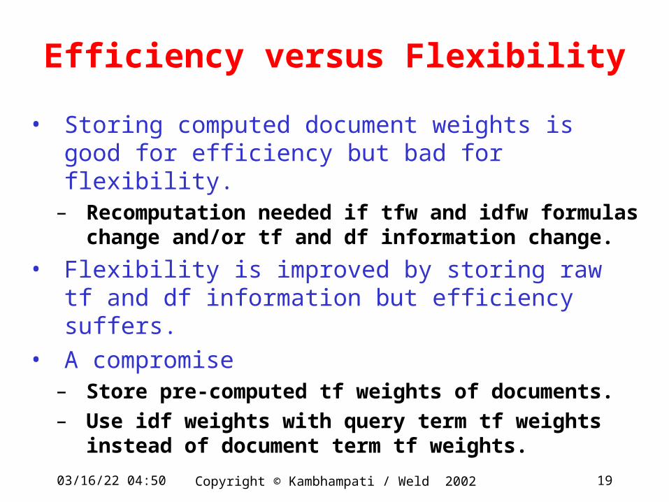
Efficiency versus Flexibility
• Storing computed document weights is good for efficiency but bad for flexibility.
– Recomputation needed if tfw and idfw formulas change and/or tf and df information change.
• Flexibility is improved by storing raw tf and df information but efficiency suffers.
• A compromise– Store pre-computed tf weights of documents.– Use idf weights with query term tf weights
instead of document term tf weights.
04/19/23 21:27 20Copyright © Kambhampati / Weld 2002
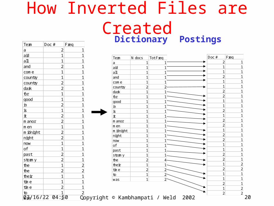
How Inverted Files are CreatedDictionary PostingsTerm Doc # Freq
a 2 1aid 1 1all 1 1and 2 1come 1 1country 1 1country 2 1dark 2 1for 1 1good 1 1in 2 1is 1 1it 2 1manor 2 1men 1 1midnight 2 1night 2 1now 1 1of 1 1past 2 1stormy 2 1the 1 2the 2 2their 1 1time 1 1time 2 1to 1 2was 2 2
Doc # Freq2 11 11 12 11 11 12 12 11 11 12 11 12 12 11 12 12 11 11 12 12 11 22 21 11 12 11 22 2
Term N docs Tot Freqa 1 1aid 1 1all 1 1and 1 1come 1 1country 2 2dark 1 1for 1 1good 1 1in 1 1is 1 1it 1 1manor 1 1men 1 1midnight 1 1night 1 1now 1 1of 1 1past 1 1stormy 1 1the 2 4their 1 1time 2 2to 1 2was 1 2
04/19/23 21:27 21Copyright © Kambhampati / Weld 2002
The Lexicon
• Grows Slowly (Heap’s law)– O(n) where n=text size; is constant ~0.4 – 0.6– E.g. for 1GB corpus, lexicon = 5Mb– Can reduce with stemming (Porter algorithm)
• Store lexicon in file in lexicographic order– Each entry points to loc in occurrence file

04/19/23 21:27 22Copyright © Kambhampati / Weld 2002
Construction
• Build Trie (or hash table)
1 6 9 11 17 19 24 28 33 40 46 50 55 60This is a text. A text has many words. Words are made from letters.
letters: 60
text: 11, 19
words: 33, 40
made: 50
many: 28
l
m ad
nt
w

04/19/23 21:27 23Copyright © Kambhampati / Weld 2002
Memory Too Small?
1 2 3 4
1-2
1-4
3-4
• Merging– When word is shared in two lexicons– Concatenate occurrence lists– O(n1 + n2)
• Overall complexity– O(n log(n/M)

04/19/23 21:27 24Copyright © Kambhampati / Weld 2002
Stop lists• Language-based stop list:
– words that bear little meaning– 20-500 words– http://www.dcs.gla.ac.uk/idom/ir_resources/linguistic_utils/stop_words
• Subject-dependent stop lists• Removing stop words
– From document– From query
From Peter Brusilovsky Univ Pittsburg INFSCI 2140
04/19/23 21:27 25Copyright © Kambhampati / Weld 2002
Stemming
• Are there different index terms?– retrieve, retrieving, retrieval, retrieved, retrieves…
• Stemming algorithm: – (retrieve, retrieving, retrieval, retrieved, retrieves)
retriev– Strips prefixes of suffixes (-s, -ed, -ly, -ness)– Morphological stemming

04/19/23 21:27 26Copyright © Kambhampati / Weld 2002
Stemming Continued • Can reduce vocabulary by ~ 1/3• C, Java, Perl versions, python, c#
www.tartarus.org/~martin/PorterStemmer
• Criterion for removing a suffix – Does "a document is about w1" mean the same as – a "a document about w2"
• Problems: sand / sander & wand / wander
04/19/23 21:27 27Copyright © Kambhampati / Weld 2002
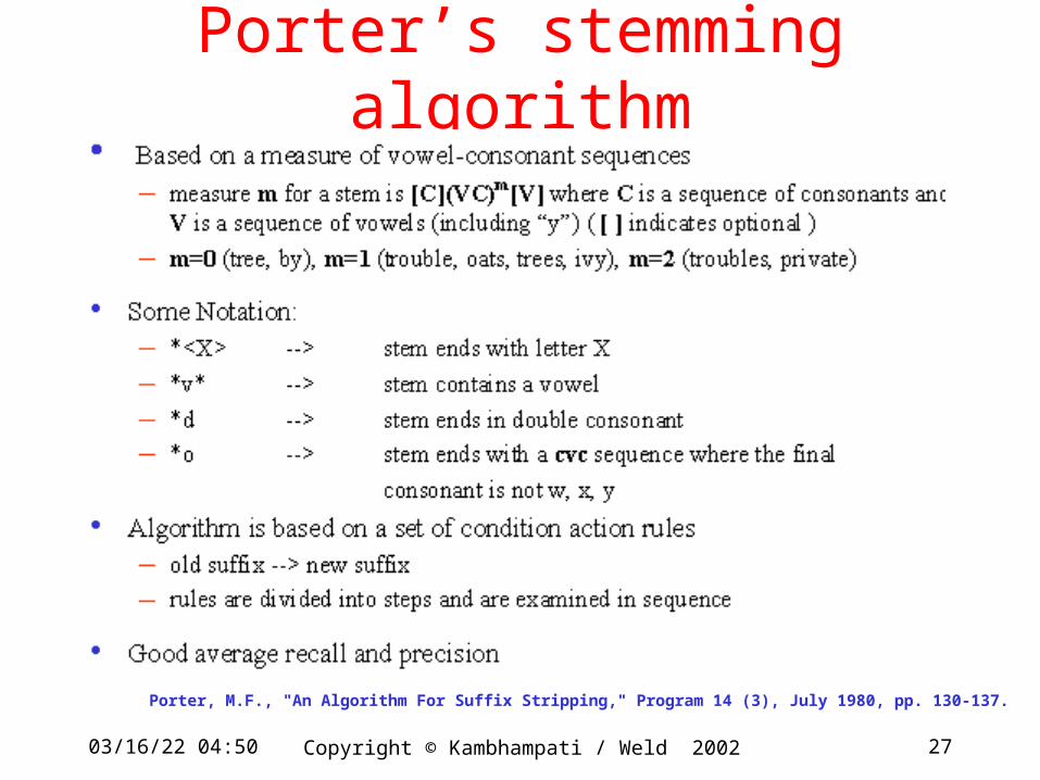
Porter’s stemming algorithm
Porter, M.F., "An Algorithm For Suffix Stripping," Program 14 (3), July 1980, pp. 130-137.
04/19/23 21:27 28Copyright © Kambhampati / Weld 2002
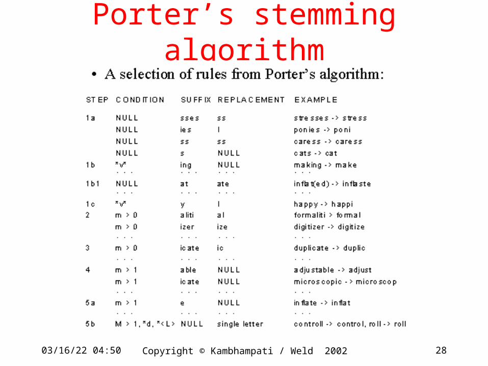
Porter’s stemming algorithm
04/19/23 21:27 29Copyright © Kambhampati / Weld 2002
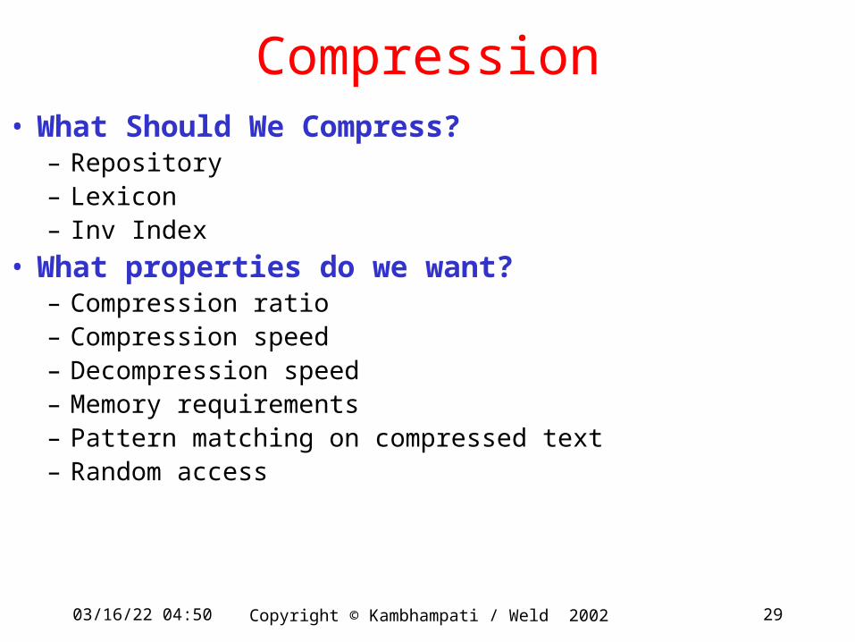
Compression• What Should We Compress?
– Repository– Lexicon– Inv Index
• What properties do we want?– Compression ratio– Compression speed– Decompression speed– Memory requirements– Pattern matching on compressed text– Random access

04/19/23 21:27 30Copyright © Kambhampati / Weld 2002
Inverted File Compression
Each inverted list has the form 1 2 3 ; , , , ... ,
tt ff d d d d
A naïve representation results in a storage overhead of ( ) * logf n N
This can also be stored as 1 2 1 1; , ,...,t tt f ff d d d d d
Each difference is called a d-gap. Since
( ) ,d gaps N each pointer requires fewer than
Trick is encoding …. since worst case ….
log N bits.
Assume d-gap representation for the rest of the talk, unless stated otherwise
Slides adapted from Tapas Kanungo and David Mount, Univ Maryland

04/19/23 21:27 31Copyright © Kambhampati / Weld 2002
Text CompressionTwo classes of text compression methods• Symbolwise (or statistical) methods
– Estimate probabilities of symbols - modeling step– Code one symbol at a time - coding step– Use shorter code for the most likely symbol– Usually based on either arithmetic or Huffman coding
• Dictionary methods– Replace fragments of text with a single code word – Typically an index to an entry in the dictionary.
• eg: Ziv-Lempel coding: replaces strings of characters with a pointer to a previous occurrence of the string.
– No probability estimates needed
Symbolwise methods are more suited for coding d-gaps

04/19/23 21:27 32Copyright © Kambhampati / Weld 2002
Classifying d-gap Compression Methods:
• Global: each list compressed using same model– non-parameterized: probability distribution for d-gap sizes is
predetermined.
– parameterized: probability distribution is adjusted according to certain parameters of the collection.
• Local: model is adjusted according to some parameter, like the frequency of the term
• By definition, local methods are parameterized.

04/19/23 21:27 33Copyright © Kambhampati / Weld 2002
Performance of index compression methods
Global methods Bible GNUbib Comact TRECUnary 262 909 487 1918Binary 15.00 16.00 18.00 20.00Bernoulli 9.86 11.06 10.90 12.30 6.51 5.68 4.48 6.63 6.23 5.08 4.35 6.38Observed Frequency 5.90 4.82 4.20 5.97
Local methods Bible GNUbib Comact TRECBernoulli 6.09 6.16 5.40 5.84Skewed Bernoulli 5.65 4.70 4.20 5.44Batched Frequency 5.58 4.64 4.02 5.41Interpolative 5.24 3.98 3.87 5.18
Compression of inverted files in bits per pointer

04/19/23 21:27 34Copyright © Kambhampati / Weld 2002
Conclusion• Local methods best• Parameterized global models ~ non-parameterized
– Pointers not scattered randomly in file
• In practice, best index compression algorithm is:
– Local Bernoulli method (using Golomb coding)• Compressed inverted indices usually faster+smaller than
– Signature files– Bitmaps
Local < Parameterized Global < Non-parameterized Global
Not by much


