4.4 GLOBAL SENSITIVITY ANALYSIS 4.4.1 GSA …€¦ · In this exercise, the permanent deformation...
91
73 4.4 GLOBAL SENSITIVITY ANALYSIS The overall goal of Global Sensitivity Analysis (GSA) is to determine sensitivity of pavement performance prediction models to the variation in the design input values. The main difference between GSA and detailed sensitivity analyses is the way the levels of an input are considered. While extreme values (only two levels) of the input ranges are considered in the detailed sensitivity analysis, GSA utilizes the entire domain for the input ranges. In this section, the details of the GSA process are presented first followed by the findings and discussion of results for the four rehabilitation options. 4.4.1 GSA Methodology The process for GSA analysis involves various steps. 1. The first step is to define a base case for all the rehabilitation options. The base cases consist of the pavement cross-section, material properties and climate information. These base cases should cover the design practices and climatic conditions in the State of Michigan. 2. The second step is to determine the ranges of input variables in order to cover the entire problem domain. 3. The third step is to sample input combinations from the problem domain. 4. The fourth step includes generating the predicted performance to the sampled inputs from the third step. 5. The fifth step involves fitting response surface models (RSM) to the generated data in step four. 6. Finally, the sensitivity metric is determined for the fitted RSM to quantify the impact of input variables on predicted performance measures. The details of the analysis related to all the above steps are presented next. 4.4.1.1. Base cases Similarly to the previously described analyses, the GSA analysis was conducted on the rehabilitation options currently used in Michigan DOT practice; i.e., HMA over HMA, HMA over PCC (composite), HMA over rubblized PCC, and unbonded PCC overlay. Also two different weather stations (Pellston and Detroit) were used to represent the effect of climate in Michigan. The effect of traffic was evaluated in the previous MDOT studies (2, 8, 9); hence in this analysis, the traffic was held constant at a typical interstate traffic level. The eight base cases evaluated in this study are shown in Table 4-40. Table 4-40 Base cases for global sensitivity analysis Rehabilitation type Climate HMA over HMA Pellston Detroit Composite (HMA over PCC) HMA over Rubblized PCC Unbonded PCC overlay
Transcript of 4.4 GLOBAL SENSITIVITY ANALYSIS 4.4.1 GSA …€¦ · In this exercise, the permanent deformation...
73
4.4 GLOBAL SENSITIVITY ANALYSIS
The overall goal of Global Sensitivity Analysis (GSA) is to determine sensitivity of
pavement performance prediction models to the variation in the design input values. The
main difference between GSA and detailed sensitivity analyses is the way the levels of an
input are considered. While extreme values (only two levels) of the input ranges are
considered in the detailed sensitivity analysis, GSA utilizes the entire domain for the input
ranges. In this section, the details of the GSA process are presented first followed by the
findings and discussion of results for the four rehabilitation options.
4.4.1 GSA Methodology
The process for GSA analysis involves various steps.
1. The first step is to define a base case for all the rehabilitation options. The base cases
consist of the pavement cross-section, material properties and climate information. These
base cases should cover the design practices and climatic conditions in the State of
Michigan.
2. The second step is to determine the ranges of input variables in order to cover the entire
problem domain.
3. The third step is to sample input combinations from the problem domain.
4. The fourth step includes generating the predicted performance to the sampled inputs from
the third step.
5. The fifth step involves fitting response surface models (RSM) to the generated data in
step four.
6. Finally, the sensitivity metric is determined for the fitted RSM to quantify the impact of
input variables on predicted performance measures.
The details of the analysis related to all the above steps are presented next.
4.4.1.1. Base cases
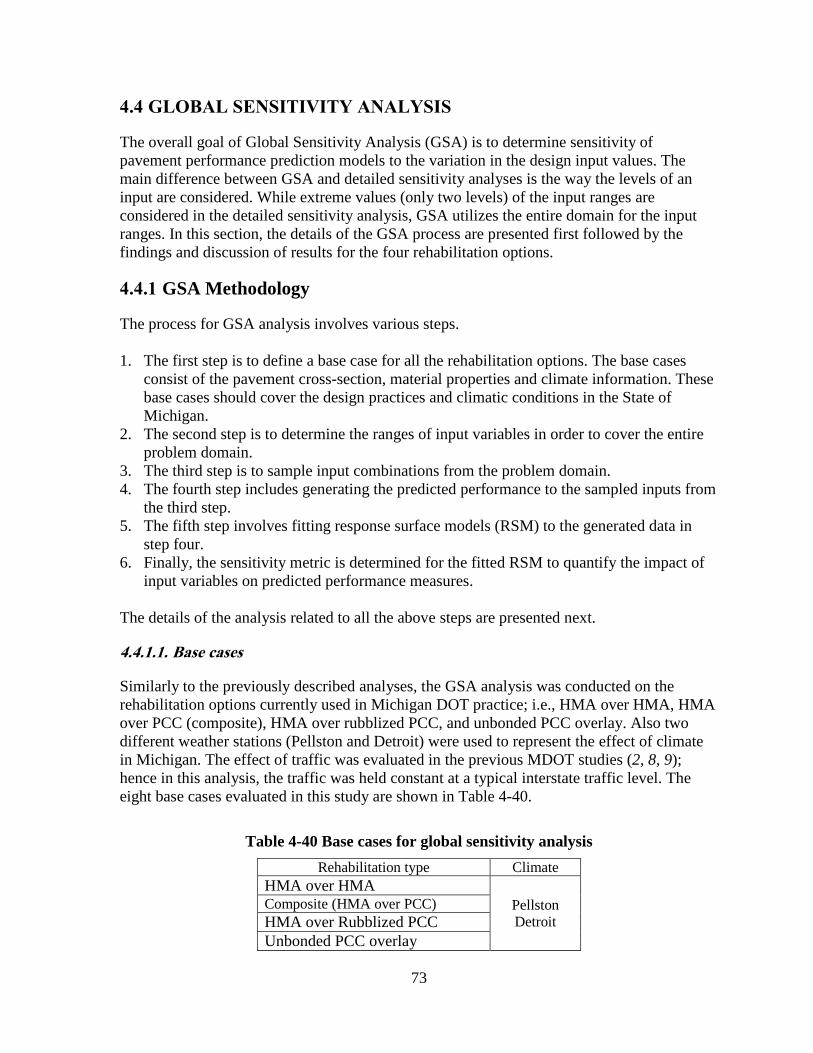
Similarly to the previously described analyses, the GSA analysis was conducted on the
rehabilitation options currently used in Michigan DOT practice; i.e., HMA over HMA, HMA
over PCC (composite), HMA over rubblized PCC, and unbonded PCC overlay. Also two
different weather stations (Pellston and Detroit) were used to represent the effect of climate
in Michigan. The effect of traffic was evaluated in the previous MDOT studies (2, 8, 9);
hence in this analysis, the traffic was held constant at a typical interstate traffic level. The
eight base cases evaluated in this study are shown in Table 4-40.
Table 4-40 Base cases for global sensitivity analysis
Rehabilitation type Climate
HMA over HMA
Pellston
Detroit
Composite (HMA over PCC)
HMA over Rubblized PCC
Unbonded PCC overlay

74
Figure 4-16 shows the climatic data for the two locations considered in the State of
Michigan. It can be observed that these climates cover different ranges of temperatures and
freezing indices.
(a) Average Freezing index by location
(b) Mean annual air temperature, number of F/T cycles and average precipitation by location
Figure 4-16 Summary of climatic properties by location within Michigan (1)
4.4.1.2. Design inputs
The MEPDG inputs represent a wide range of categories including traffic characterization,
climatic data, and pavement structural and material information. Some of the inputs related to
material characterization need special considerations. For example, characterizing existing
pavement damage involves different input levels for the HMA over HMA rehabilitation
option. Therefore, some decisions are needed to determine the specific input for the selected
75
level. The following section presents some of such cases for HMA over HMA rehabilitation
option.
Characterizing HMA over HMA layer
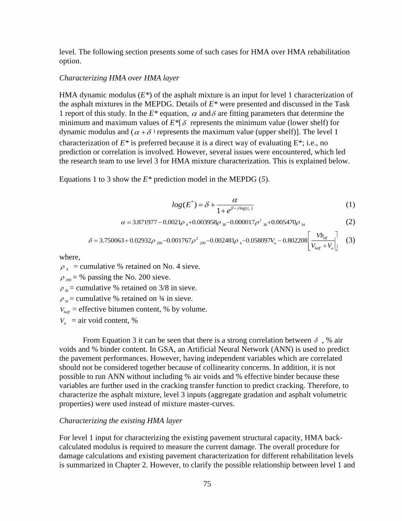
HMA dynamic modulus (E*) of the asphalt mixture is an input for level 1 characterization of
the asphalt mixtures in the MEPDG. Details of E* were presented and discussed in the Task
1 report of this study. In the E* equation, and are fitting parameters that determine the
minimum and maximum values of E*[ represents the minimum value (lower shelf) for
dynamic modulus and ( ) represents the maximum value (upper shelf)]. The level 1
characterization of E* is preferred because it is a direct way of evaluating E*; i.e., no
prediction or correlation is involved. However, several issues were encountered, which led
the research team to use level 3 for HMA mixture characterization. This is explained below.
Equations 1 to 3 show the E* prediction model in the MEPDG (5).
*
log( )( )
1 rtlog E
e
(1)
2
4 38 38 343.871977 0.0021 0.003958 0.000017 0.005470 (2)
2
200 200 43.750063 0.02932 0.001767 0.002481 0.058097 0.802208eff
a
beff a
VbV
V V
(3)
where,
4 = cumulative % retained on No. 4 sieve.
200 = % passing the No. 200 sieve.
38 = cumulative % retained on 3/8 in sieve.
34 = cumulative % retained on ¾ in sieve.
beffV = effective bitumen content, % by volume.
aV = air void content, %
From Equation 3 it can be seen that there is a strong correlation between , % air
voids and % binder content. In GSA, an Artificial Neural Network (ANN) is used to predict
the pavement performances. However, having independent variables which are correlated
should not be considered together because of collinearity concerns. In addition, it is not
possible to run ANN without including % air voids and % effective binder because these
variables are further used in the cracking transfer function to predict cracking. Therefore, to
characterize the asphalt mixture, level 3 inputs (aggregate gradation and asphalt volumetric
properties) were used instead of mixture master-curves.
Characterizing the existing HMA layer
For level 1 input for characterizing the existing pavement structural capacity, HMA back-
calculated modulus is required to measure the current damage. The overall procedure for
damage calculations and existing pavement characterization for different rehabilitation levels
is summarized in Chapter 2. However, to clarify the possible relationship between level 1 and

76
level 3 rehabilitation levels, the amount of overlay cracking was obtained using the MEPDG
for these levels. In this exercise, the permanent deformation input was kept constant while
the pavement condition rating was varied to determine the corresponding back-calculated
modulus to produce the same amount of cracking. Thin (3 in) and thick (6 in) overlays were
used for the comparison and the results are shown in Figures 4-17 and 4-18. The results show
that each pavement condition rating corresponds to a specific range of the existing HMA
back-calculated moduli. For example, very poor condition rating for an existing pavement
corresponds to 250 ksi modulus as both rehabilitation levels exhibited the same amount of
longitudinal and alligator cracking regardless of the overlay thickness. On the other hand, a
modulus of 600 ksi for existing HMA yielded the same amount of cracking similar to
excellent pavement condition rating. Based on these results, it is possible to relate the level 3
existing pavement condition ratings with the level 1 back-calculated moduli of the existing
HMA layer. Therefore, in this study level 3 rehabilitation was utilized in all analyses. Also, if
there is a fair estimate of the existing pavement modulus, level 3 (pavement condition rating)
can be used instead of the level 1 (back-calculated modulus).
(a) Longitudinal cracking for 6 in overlay
(b) Longitudinal cracking for 3 in overlay
Figure 4-17 Comparison between levels 1 and 3 rehabilitation for longitudinal cracking
(a) Fatigue cracking for 6 in overlay
(b) Fatigue cracking for 3 in overlay
Figure 4-18 Comparison between levels 1 and 3 rehabilitation for fatigue cracking
0
500
1000
1500
2000
2500
3000
3500
4000
Cra
ckin
g (
ft/m
ile)
Level 1
Level 3
0
1000
2000
3000
4000
5000
6000
7000
8000
9000
10000
Cra
ckin
g (
ft/m
ile)
Level 1
Level 3
0
0.5
1
1.5
2
2.5
3
3.5
4
Cra
ckin
g (
% c
rack
ed a
rea)
Level 1
Level 3
0
2
4
6
8
10
12
14
16
18
20
Cra
ckin
g (
% c
rack
ed a
rea) Level 1
Level 3

77
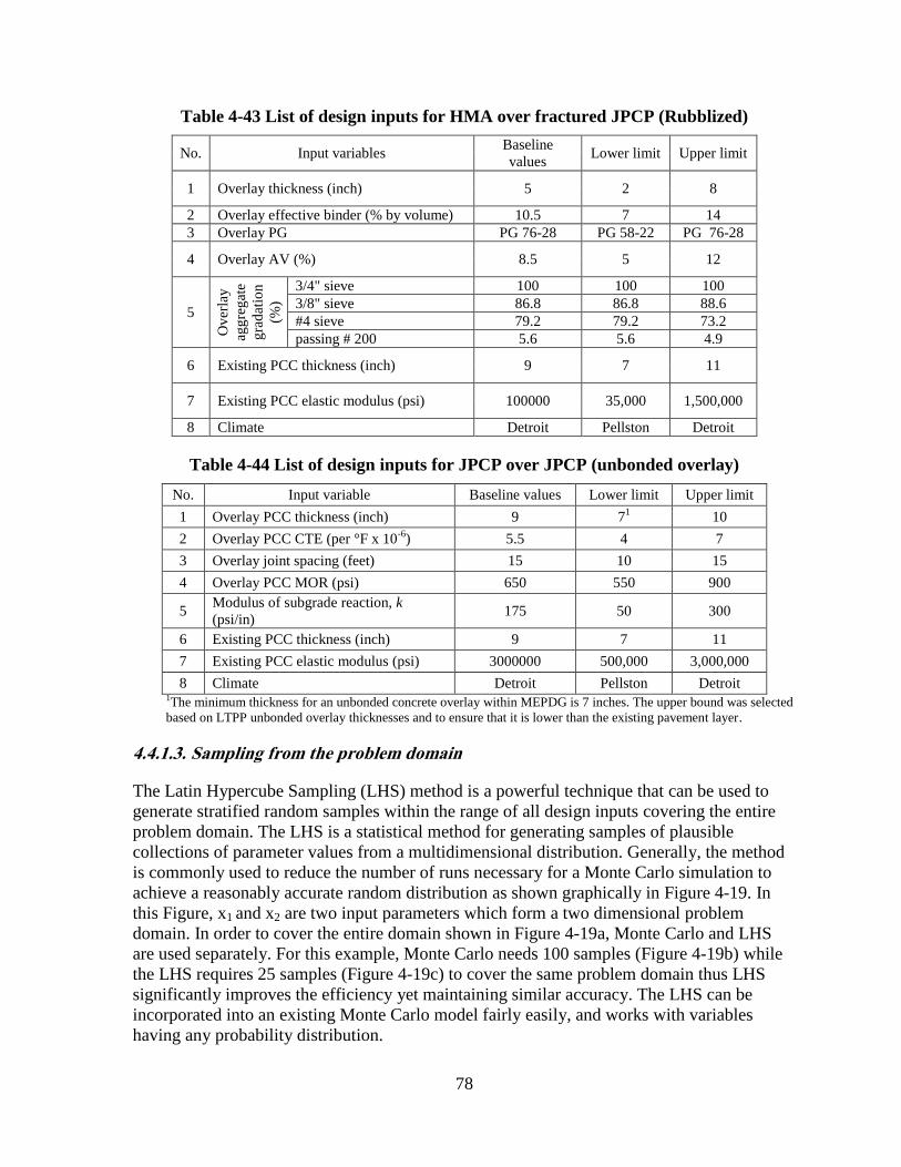
Rehabilitation options design inputs and ranges
The results of the preliminary sensitivity analysis were used here to determine the potentially
significant inputs for different rehabilitation options. The final list of design inputs and their
ranges were finalized with MDOT. Tables 4-41 to 4-44 summarize the design inputs, their
ranges, and the baseline values for all rehabilitation options considered in this study. For the
one-at-a-time (OAT) sensitivity analysis, the value of each input variable was varied over its
entire range (from lower to upper limits) while all other input variables were held constant at
their baseline values.
Table 4-41 List of design inputs for HMA over HMA
No. Input variables Baseline values Lower limit Upper limit
1 Overlay thickness (inch) 5 2 8
2 Overlay effective binder (% by volume) 10.5 7 14
3 Overlay PG PG 58-221 PG 58-22 PG 76-28
4 Overlay AV (%) 8.5 5 12
5
Ov
erla
y
agg
reg
ate
gra
dat
ion
(%)
3/4" sieve 100 100 100
3/8" sieve 88.6 86.8 88.6
#4 sieve 73.2 79.2 73.2
passing # 200 4.9 5.6 4.9
6 Existing condition rating Poor Very poor Excellent
7 Existing HMA thickness (inch) 8 4 12
8 Existing base modulus (psi) 27500 15000 40000
9 Existing Sub-base modulus (psi) 20000 15000 30000
10 Subgrade modulus (psi) 13750 2500 25000
11 Climate Pellston2 Pellston Detroit
Table 4-42 List of design inputs for composite
No. Input variables Baseline values Lower limit Upper limit
1 Overlay thickness (inch) 5 2 8
2 Overlay effective binder (% by volume) 10.5 7 14
3 Overlay PG PG 76-28 PG 58-22 PG 76-28
4 Overlay AV (%) 8.5 5 12
5
Ov
erla
y
agg
reg
ate
gra
dat
ion
(%)
100 100 100 100
88.6 86.8 86.8 88.6
73.2 79.2 79.2 73.2
4.9 5.6 5.6 4.9
6 Existing PCC thickness (inch) 9 7 11
7 Existing PCC MOR (psi) 650 550 900
8 Subgrade reaction modulus (psi/in) 175 50 300
9 Climate Detroit Pellston Detroit
1 Only two levels for PG were considered; therefore, the baseline value is identical to the lower limit.
2 Pellston was used as a baseline in this case.
78
Table 4-43 List of design inputs for HMA over fractured JPCP (Rubblized)
No. Input variables Baseline
values Lower limit Upper limit
1 Overlay thickness (inch) 5 2 8
2 Overlay effective binder (% by volume) 10.5 7 14
3 Overlay PG PG 76-28 PG 58-22 PG 76-28
4 Overlay AV (%) 8.5 5 12
5
Ov
erla
y
agg
reg
ate
gra
dat
ion
(%)
3/4" sieve 100 100 100
3/8" sieve 86.8 86.8 88.6
#4 sieve 79.2 79.2 73.2
passing # 200 5.6 5.6 4.9
6 Existing PCC thickness (inch) 9 7 11
7 Existing PCC elastic modulus (psi) 100000 35,000 1,500,000
8 Climate Detroit Pellston Detroit
Table 4-44 List of design inputs for JPCP over JPCP (unbonded overlay)
No. Input variable Baseline values Lower limit Upper limit
1 Overlay PCC thickness (inch) 9 71
10
2 Overlay PCC CTE (per °F x 10-6
) 5.5 4 7
3 Overlay joint spacing (feet) 15 10 15
4 Overlay PCC MOR (psi) 650 550 900
5 Modulus of subgrade reaction, k
(psi/in) 175 50 300
6 Existing PCC thickness (inch) 9 7 11
7 Existing PCC elastic modulus (psi) 3000000 500,000 3,000,000
8 Climate Detroit Pellston Detroit 1The minimum thickness for an unbonded concrete overlay within MEPDG is 7 inches. The upper bound was selected
based on LTPP unbonded overlay thicknesses and to ensure that it is lower than the existing pavement layer.
4.4.1.3. Sampling from the problem domain
The Latin Hypercube Sampling (LHS) method is a powerful technique that can be used to
generate stratified random samples within the range of all design inputs covering the entire
problem domain. The LHS is a statistical method for generating samples of plausible
collections of parameter values from a multidimensional distribution. Generally, the method
is commonly used to reduce the number of runs necessary for a Monte Carlo simulation to
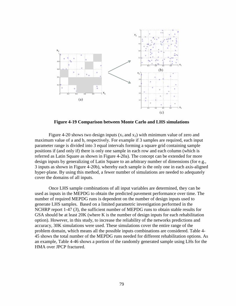
achieve a reasonably accurate random distribution as shown graphically in Figure 4-19. In
this Figure, x1 and x2 are two input parameters which form a two dimensional problem
domain. In order to cover the entire domain shown in Figure 4-19a, Monte Carlo and LHS
are used separately. For this example, Monte Carlo needs 100 samples (Figure 4-19b) while
the LHS requires 25 samples (Figure 4-19c) to cover the same problem domain thus LHS
significantly improves the efficiency yet maintaining similar accuracy. The LHS can be
incorporated into an existing Monte Carlo model fairly easily, and works with variables
having any probability distribution.
79
Figure 4-19 Comparison between Monte Carlo and LHS simulations
Figure 4-20 shows two design inputs (x1 and x2) with minimum value of zero and
maximum value of a and b, respectively. For example if 3 samples are required, each input
parameter range is divided into 3 equal intervals forming a square grid containing sample
positions if (and only if) there is only one sample in each row and each column (which is
referred as Latin Square as shown in Figure 4-20a). The concept can be extended for more
design inputs by generalizing of Latin Square to an arbitrary number of dimensions (for e.g.,
3 inputs as shown in Figure 4-20b), whereby each sample is the only one in each axis-aligned
hyper-plane. By using this method, a fewer number of simulations are needed to adequately
cover the domains of all inputs.
Once LHS sample combinations of all input variables are determined, they can be
used as inputs in the MEPDG to obtain the predicted pavement performance over time. The
number of required MEPDG runs is dependent on the number of design inputs used to
generate LHS samples. Based on a limited parametric investigation performed in the
NCHRP report 1-47 (3), the sufficient number of MEPDG runs to obtain stable results for
GSA should be at least 20K (where K is the number of design inputs for each rehabilitation
option). However, in this study, to increase the reliability of the networks predictions and
accuracy, 30K simulations were used. These simulations cover the entire range of the
problem domain, which means all the possible inputs combinations are considered. Table 4-
45 shows the total number of the MEPDG runs needed for different rehabilitation options. As
an example, Table 4-46 shows a portion of the randomly generated sample using LHs for the
HMA over JPCP fractured.

80
(a) Latin Square
(b) Latin Cube
Figure 4-20 Example of sampling in LHS method
Table 4-45 Required number of simulations
Rehabilitation type Number of inputs Number of runs
HMA over HMA 11 330
HMA over PCC (Composite) 9 270
HMA over Rubblized PCC 8 240
Unbonded PCC overlay 8 240
Table 4-46 Generated samples for HMA over JPCP fractured
Run Overlay
Thickness
Overlay
Effective
Binder
Overlay
PG
Overlay
Air
Voids
Overlay
Aggregate
Existing
Thickness
Existing
Thickness Climate
1 3.188 12.952 PG 76-28 6.489 Coarse 9.636 50924 Pellston
2 5.585 10.358 PG 76-28 11.371 Coarse 10.903 683920 Detroit
3 7.118 10.002 PG 76-28 5.864 Coarse 10.794 412611 Pellston
. . . . . . . . .
. . . . . . . . .
236 7.587 13.136 PG 58-22 7.946 Coarse 7.498 949310 Pellston
237 3.933 10.191 PG 76-28 5.298 Coarse 9.244 499617 Pellston
238 3.634 11.373 PG 58-22 10.032 Fine 7.691 475511 Detroit
239 6.086 7.794 PG 76-28 6.936 Coarse 8.153 142600 Pellston
240 7.703 11.393 PG 76-28 8.179 Coarse 9.332 1249368 Pellston

81
4.4.1.4. Response surface models (RSM)
The LHS generated input combinations (which are essentially random MEPDG design input
scenarios) were used to make the MEPDG input files. The pavement performance prediction
results were obtained after executing these input files using the MEPDG (version1.1). These
results were used to provide a continuous surface of pavement performance at discrete
locations in the problem domain. However, to obtain continuous performance measures other
than the predefined discrete locations, a continuous surface should be fitted on these discrete
points. Therefore, Artificial Neural Network (ANN) fitting tools were used to fit continuous
surfaces. ANN consists of an interconnected group of artificial neurons, and it processes
information using a connectionist approach for computation. Neural networks are used to
model complex relationships between inputs and outputs or to find patterns in data. The
ANN can be viewed as a nonlinear regression model except that the functional form of the
fitting equation does not need to be specified necessarily (3). Subsequently, the RSMs
estimated by using ANN were utilized to calculate sensitivity of different design inputs using
the sensitivity metric called Normalized Sensitivity Index (NSI).
4.4.1.5. Sensitivity metric
The NSI can be used for a point estimation of sensitivity across a problem domain. The
point-normalized sensitivity index ijkS is defined as:
j ki
ijk
k jii
dy xS
dx y (4)
where,
kix is the value of input k at point i
jiy is the value of distress j at point i
j
k i
dy
dxis change of distress j with respect to change in input k at point i
Equation (4) can be simplified to:
j
j
ijkk
ki
dy
yS
dx
x
(5)
Equation (5) shows that the sensitivity index is a ratio between rates of change in
performance measure and design input. In some cases, predicted distress, jiy is close to zero
resulting in an artificially large sensitivity. Therefore, to overcome this problem ijkS can be

82
normalized with the design limit for a distress. The final formula for sensitivity index is as
follows (3):
jiDL ki
ijk
ki j
y xNSI S
x DL
(6)
where,
NSI is normalized sensitivity index for design limit at point i for distress j and input k
jiy is change in distress j about point i
kix is change in input k about point i
kix is the value of input k at point i
jDL is the design limit for distress j
The NSI was calculated using Equation (6) for most of the cases. However, for
discrete design inputs (for e.g., climate, condition rating, PG grade etc.), a modified equation
was implemented to determine the sensitivity index. Equation (7) still considers the design
limit as reference for predicted distress; it normalizes the change in the performance with
respect to the specified design limit for a certain distress if the design input is changed by one
category. For example, if by changing PG grade from PG 58-22 to PG 76-28 rutting changes
by 0.7 inches while all other inputs are held constant, the NSI for rutting will be 0.7/0.5=1.4.
It should be noted that the difference in the predicted performance between categories should
be higher than the threshold to obtain NSI greater than 1 to consider the input as significant.
1ki
ji
j X category
yNSI
DL
(7)
The NSI for IRI also needs special attention because the lower bound for IRI is non-
zero. The NSI formula for IRI when the design limit is 172 inch/mile and the initial IRI is 63
inch/mile is expressed in Equation (8). This equation was proposed in the NCHRP 1-47 study
for performing the sensitivity analysis.
63
172 63
IRINSI
(8)
The NSI can be interpreted as:
If NSI=0, then there is no change in performance with respect to the change in input,
If NSI=1, then the rates of change in performance and input are the same,
If NSI >1, the performance rate of change is faster than the rate of change in the
input.
The NSI interpretation is for OAT analysis, and only explains the main effect of an
input on a given distress measure. Therefore, there was a need to explain the interactive
effect of two variables for evaluating the joint effect of variables. Equations (9) and (10)
were developed to evaluate NSI of an interaction where Equation (11) shows the numerical
solution for Equation (10).

83
2
( , )( , )
m k l
ijklm k l mi ji j
y x xS
x x y
(9)
2
( , )( , )
ijklm
m k lDL
k l mi j
i j
y x xNSI
x x DL
(10)
1 1 1 1, , , ,
( , )
k l k l k l k li j i ji j j i
m m m mk l
x x x x x x x xi jDLijklm mk li j
i j
y y y yx xNSI S
DLx x
(11)
where,
( , )
DL
ijklm i jS =
sensitivity index for input k and l, distress m, at point (i,j) with respect to
design limit (DL) kix = value of input kx at point i
ljx = value of input lx at point j
k
ix = change in input kx around point i 1 1
k k
i ix x
l
jx = change in input lx around point j 1 1
l l
j jx x
,k li j
m
x xy = value of distress m, for input kx at point i and input lx at point j
mDL = design limit for distress m
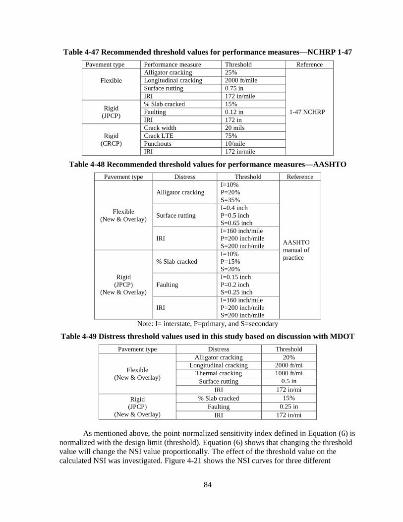
4.4.1.6. Distress thresholds for GSA
The NSI calculation involves the design limit (threshold value) for each distress type.
Tables 4-47 and 4-48 summarize recommended threshold values for various performance
measures from the NCHRP Report 1-47(3) and MEPDG manual of practice (10),
respectively . It should be noted that practically, the distress threshold values depend on the
road class, and may vary among agencies based on their practices. Finally, Table 4-49
summarizes the threshold values adopted in this study based on discussions with MDOT
(January 7, 2013).
84
Table 4-47 Recommended threshold values for performance measures—NCHRP 1-47
Pavement type Performance measure Threshold Reference
Flexible
Alligator cracking 25%
1-47 NCHRP
Longitudinal cracking 2000 ft/mile
Surface rutting 0.75 in
IRI 172 in/mile
Rigid
(JPCP)
% Slab cracked 15%
Faulting 0.12 in
IRI 172 in
Rigid
(CRCP)
Crack width 20 mils
Crack LTE 75%
Punchouts 10/mile
IRI 172 in/mile
Table 4-48 Recommended threshold values for performance measures—AASHTO
Pavement type Distress Threshold Reference
Flexible
(New & Overlay)
Alligator cracking
I=10%
P=20%
S=35%
AASHTO
manual of
practice
Surface rutting
I=0.4 inch
P=0.5 inch
S=0.65 inch
IRI
I=160 inch/mile
P=200 inch/mile
S=200 inch/mile
Rigid
(JPCP)
(New & Overlay)
% Slab cracked
I=10%
P=15%
S=20%
Faulting
I=0.15 inch
P=0.2 inch
S=0.25 inch
IRI
I=160 inch/mile
P=200 inch/mile
S=200 inch/mile
Note: I= interstate, P=primary, and S=secondary
Table 4-49 Distress threshold values used in this study based on discussion with MDOT
Pavement type Distress Threshold
Flexible
(New & Overlay)
Alligator cracking 20%
Longitudinal cracking 2000 ft/mi
Thermal cracking 1000 ft/mi
Surface rutting 0.5 in
IRI 172 in/mi
Rigid
(JPCP)
(New & Overlay)
% Slab cracked 15%
Faulting 0.25 in
IRI 172 in/mi
As mentioned above, the point-normalized sensitivity index defined in Equation (6) is
normalized with the design limit (threshold). Equation (6) shows that changing the threshold
value will change the NSI value proportionally. The effect of the threshold value on the
calculated NSI was investigated. Figure 4-21 shows the NSI curves for three different

85
threshold values. The results show that the change in threshold value will proportionally
increase or decrease the NSI value for a given performance measure.
(a) Alligator cracking for HMA over HMA
(b) Surface rutting for HMA over HMA
(c) Roughness (IRI) for HMA over HMA
Figure 4-21 Effect of different threshold values on NSI calculation
2 3 4 5 6 7 8-2.5
-2
-1.5
-1
-0.5
0
Overlay thickness
NS
I
Alligator cracking NSI
Design Limit=10%
Design Limit=20%
Design Limit=35%
2 3 4 5 6 7 8-1.4
-1.3
-1.2
-1.1
-1
-0.9
-0.8
-0.7
-0.6
-0.5
-0.4
Overlay thickness
NS
I
Rutting NSI
Design Limit=0.4 in
Design Limit=0.5 in
Design Limit=0.65 in

86
4.4.2 Global Sensitivity Analysis Results
In GSA, for each rehabilitation option both main and interactive effects of inputs on
pavement distresses were investigated. More than 1000 ANN RSMs were performed for each
input-distress combination and the RSMs were averaged to obtain an expected RSM to
improve the accuracy of performance predictions. Subsequently, those RSMs were utilized to
evaluate the NSI. Due to the variation in the ANN predictions for 1000 RSMs, a 95%
confidence interval was provided for distress and NSI predictions. The GSA included the
following components for each rehabilitation option:
1. The relative importance of design inputs were determined by using the Garson
algorithm.
2. The main effects of each design input were evaluated by using NSI values.
3. The interaction effects of important design inputs were evaluated by using two-
variable NSI values.
The results for each rehabilitation option are presented next.
4.4.2.1. HMA over HMA
Relative importance of design inputs
In order to obtain the overall relative significance of design inputs, all the inputs should be
changed simultaneously to cover their entire possible combinations. Therefore, in this case
despite an OAT analysis (where all results are based on a base case), no base case or baseline
values for design inputs are needed. However, it should be noted that such methodology only
determines the relative ranking of inputs among each other. Garson algorithm was
implemented to get the relative importance of the design inputs. Garson (11) proposed a
method for partitioning the neural network connection weights in order to determine the
relative importance of each input variable in the network. An example showing the
application of Garson’s algorithm in a single hidden layer feed forward multi-layer
perceptron (MLP) with two processing elements (PEs) is shown in Figure 4-22.
Figure 4-22 Network diagram (11)

87
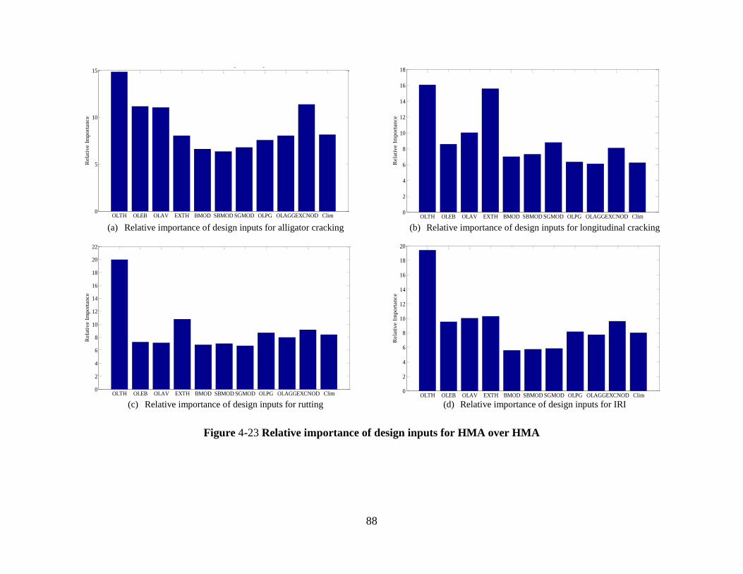
The dataset used in this analysis are the LHS inputs generated for GSA. The LHS inputs
cover the entire range of problem domain hence it takes into account all the possible input
combinations. The relative importance of the design inputs is shown in Figure 4-23 for all
pavement performance measures. The relative importance of an input can also be expressed
as the percent participation of design inputs in the distress prediction models (i.e. for a given
pavement distress each design input will have a percent contribution to the predicted
distress). The results show that overlay thickness is the most important input and has the
highest contribution in all predicted performance measures. The volumetric parameters for
overlay HMA mixture (effective binder and air voids) are important for cracking, especially
for alligator cracking. Existing condition rating for alligator cracking and existing HMA
thickness for longitudinal cracking and rutting have important overall contributions.
The height of each bar graph shows the percent contribution of the input parameters
(which adds up to 100%). In general, these numbers can be used to compare and quantify the
contributions of each input for a specific performance measure.
88
(a) Relative importance of design inputs for alligator cracking
(b) Relative importance of design inputs for longitudinal cracking
(c) Relative importance of design inputs for rutting
(d) Relative importance of design inputs for IRI
Figure 4-23 Relative importance of design inputs for HMA over HMA
OLTH OLEB OLAV EXTH BMOD SBMOD SGMOD OLPG OLAGGEXCNOD Clim0
5
10
15
Rela
tiv
e I
mp
ort
an
ce
HMA over HMA - Alligator cracking
OLTH OLEB OLAV EXTH BMOD SBMOD SGMOD OLPG OLAGGEXCNOD Clim0
2
4
6
8
10
12
14
16
18
Rela
tive I
mport
ance
HMA over HMA - Longitudinal cracking
OLTH OLEB OLAV EXTH BMOD SBMOD SGMOD OLPG OLAGGEXCNOD Clim0
2
4
6
8
10
12
14
16
18
20
22
Rela
tiv
e I
mp
ort
an
ce
HMA over HMA - Rutting
OLTH OLEB OLAV EXTH BMOD SBMOD SGMOD OLPG OLAGGEXCNOD Clim0
2
4
6
8
10
12
14
16
18
20
Rela
tive I
mport
ance
HMA over HMA - IRI
89
Main effect of design inputs
As mentioned above, the relative importance of inputs can be used for determining their overall
contribution to predicted pavement performance. In order to investigate the impact of the input
variables with respect to a standard, a base case should be specified. In this scenario, each input
variable of interest should vary over its range while other variables are held constant at their base
values. The base cases, input ranges, and baseline values were presented before.
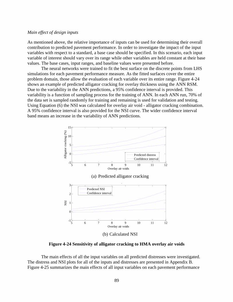
The neural networks were trained to fit the best surface on the discrete points from LHS
simulations for each pavement performance measure. As the fitted surfaces cover the entire
problem domain, those allow the evaluation of each variable over its entire range. Figure 4-24
shows an example of predicted alligator cracking for overlay thickness using the ANN RSM.
Due to the variability in the ANN predictions, a 95% confidence interval is provided. This
variability is a function of sampling process for the training of ANN. In each ANN run, 70% of
the data set is sampled randomly for training and remaining is used for validation and testing.
Using Equation (6) the NSI was calculated for overlay air void - alligator cracking combination.
A 95% confidence interval is also provided for the NSI curve. The wider confidence interval
band means an increase in the variability of ANN predictions.
(a) Predicted alligator cracking
(b) Calculated NSI
Figure 4-24 Sensitivity of alligator cracking to HMA overlay air voids
The main effects of all the input variables on all predicted distresses were investigated.
The distress and NSI plots for all of the inputs and distresses are presented in Appendix B.
Figure 4-25 summarizes the main effects of all input variables on each pavement performance
5 6 7 8 9 10 11 12-5
0
5
10
15
Overlay air voids
All
igat
or
crac
kin
g (
%)
Alligator cracking vs. Overlay air voids
Predicted distress
Confidence interval
5 6 7 8 9 10 11 12-1
0
1
2
3
Overlay air voids
NS
I
NSI vs. Overlay air voids
Predicted NSI
Confidence interval
5 6 7 8 9 10 11 12-5
0
5
10
15
Overlay air voids
All
igat
or
crac
kin
g (
%)
Alligator cracking vs. Overlay air voids
Predicted distress
Confidence interval
5 6 7 8 9 10 11 12-1
0
1
2
3
Overlay air voids
NS
I
NSI vs. Overlay air voids
Predicted NSI
Confidence interval

90
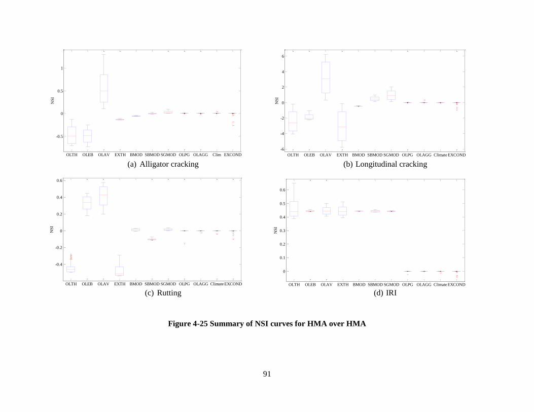
measure by box plots. The results show that overlay air void percentage has a significant impact
on cracking (NSI>1). An increase in air voids is associated with higher cracking. For
longitudinal cracking; overlay and existing HMA thickness, effective binder content, unbound
layer moduli and existing conditions all have a significant impact. The effect of a particular input
on pavement performance measure can be interpreted as follows:
If a NSI is positive, the distress magnitude will increase by increasing the input
value.
If a NSI is negative, the distress magnitude will decrease by increasing the input
value.
For rutting and IRI, the NSI results show that all inputs have relatively lower impact as
compared to cracking.
Interactive effect of design inputs
The detailed sensitivity analysis identified some practically significant interactions between input
variables. Those interactions were further investigated in detail in this part. An interactive effect
means that one input can amplify or reduce the effect of another input on the predicted pavement
performance. Therefore, it is vital to consider the interactive effect of given design input
variables when such interaction exists. It should be noted that only interactions between overlay
design and existing design inputs were considered. Similar to the NSI for one variable, a NSI for
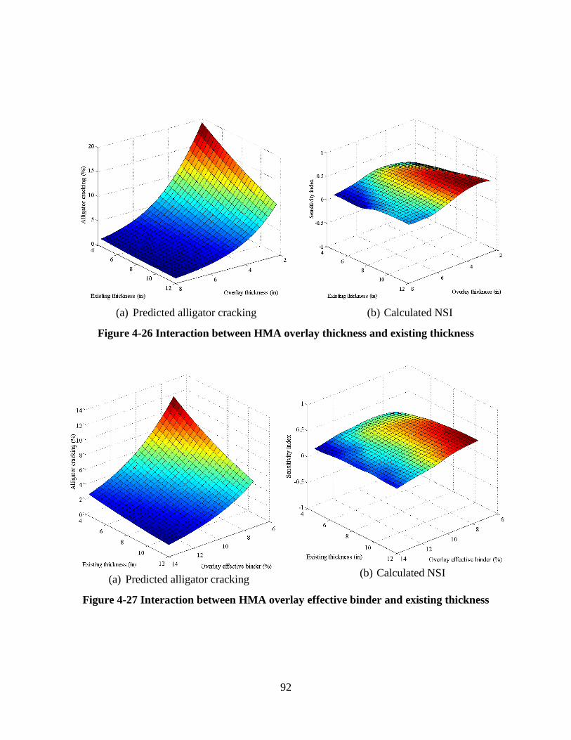
interaction was developed as shown in Equation (11). Figures 4-26 to 4-28 show the significant
interactions for alligator cracking and the corresponding NSI plots. The results shown in Figure
4-26a indicates that higher overlay thicknesses lower the impact of existing thickness on alligator
cracking. For example, for an 8-inch overlay thickness, regardless of the existing HMA
thickness, the predicted cracking will be negligible over the design life. On the other hand, for a
thin overlay depending on the existing HMA thickness, the rehabilitation strategy will exhibit 10
to 20% alligator cracking over the design life. Figure 4-26b shows that the rate of change in
cracking with respect to overlay thickness will increase as the existing thickness increases.
Other interactions in Figures 4-27 and 4-28 can be interpreted similarly. The maximum
NSI for interactions can be used to rank the interactions. The results for alligator cracking of
HMA over HMA as shown in Figure 4-26 to Figure 4-28 manifests that the interaction between
overlay air voids and existing HMA thickness has the most important effect. The interaction
between existing thickness and overlay thickness, and existing thickness and overlay effective
binder content have somewhat similar effects on alligator cracking. It should be noted that in the
interaction sensitivity plots, the magnitude of the NSI should be consider rather than the surface
colors.
On each boxplot, the central mark (red line) is the median of the distribution; the lower
and upper edges of the box are the 25th and 75th percentiles, respectively. The whiskers extend
to the most extreme data points without considering outliers, and outliers are plotted individually
as the red plus signs in the graph. It should be noted that box plots are used for continuous
variables to represent a continuous distribution and do not apply to discrete variables.
91
(a) Alligator cracking
(b) Longitudinal cracking
(c) Rutting
(d) IRI
Figure 4-25 Summary of NSI curves for HMA over HMA
OLTH OLEB OLAV EXTH BMOD SBMOD SGMOD OLPG OLAGG Clim EXCOND
-0.5
0
0.5
1
NS
I
HMA over HMA - Alligator cracking
OLTH OLEB OLAV EXTH BMOD SBMOD SGMOD OLPG OLAGG Climate EXCOND
-6
-4
-2
0
2
4
6
NS
I
HMA over HMA - Longitudinal cracking
OLTH OLEB OLAV EXTH BMOD SBMOD SGMOD OLPG OLAGG Climate EXCOND
-0.4
-0.2
0
0.2
0.4
0.6
NS
I
HMA over HMA - Rutting
OLTH OLEB OLAV EXTH BMOD SBMOD SGMOD OLPG OLAGG Climate EXCOND
0
0.1
0.2
0.3
0.4
0.5
0.6
NS
I
HMA over HMA - IRI
92
(a) Predicted alligator cracking
(b) Calculated NSI
Figure 4-26 Interaction between HMA overlay thickness and existing thickness
(a) Predicted alligator cracking
(b) Calculated NSI
Figure 4-27 Interaction between HMA overlay effective binder and existing thickness

93
(a) Predicted alligator cracking
(b) Calculated NSI
Figure 4-28 Interaction between HMA overlay air voids and existing thickness
4.4.2.2. Composite pavement
Relative importance of design inputs
Similar to HMA overlay, the relative importance of design inputs for this rehabilitation option is
determined as shown in Figure 4-29. Since no alligator cracking was predicted by the MEPDG,
the results are only shown for the remaining distresses. The results demonstrate the overlay
thickness and overlay air voids have the highest contribution to all the predicted pavement
performance measures. The volumetric parameters for overlay HMA mixture (effective binder
content, air voids, and aggregate gradation) and PG grade are important for rutting and have
somewhat similar contributions.
Main effect of design inputs
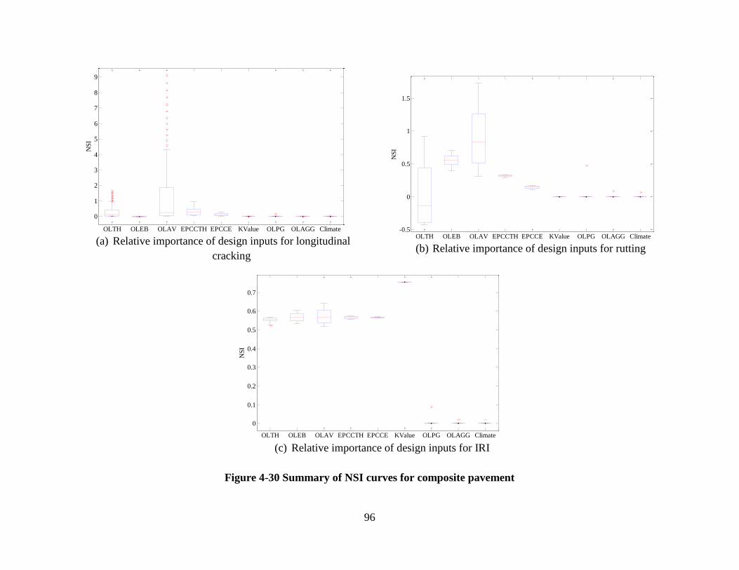
The summary of NSI plots for composite pavements is presented in Figure 4-30. The results
show that the overlay thickness and overlay air voids have the highest impact on all predicted
distress among design inputs. Existing PCC thickness has an important effect on longitudinal
cracking. The NSI results show that all inputs have relatively lower impact on IRI as compared
to cracking and rutting. The plots were generated using more than 100 points within the ranges
of the design inputs; therefore, some of the inputs (e.g., OLAV) might show a noticeable number
of outliers. However, such outliers were much less than the total number of data point for
generating these plots. It should be noted that box plot summarizes a NSI curve for each design
input range. In some cases if there is a rapid change in NSI due to a specific input value, the
point will be shown as an outlier in the box plot (see Figure B-59 for overlay air voids NSI).
Therefore, the maximum value of NSI was used as the criteria for identifying a significant input
variable.

94
Interactive effect of design inputs
Interaction effects between input variables and NSI for this rehabilitation option are presented in
Appendix B. Figures B-66 and B-67 show significant interactions for longitudinal cracking. The
results show that thinner overlay will lower the impact of existing thickness on longitudinal
cracking. For example, for a 2-inch overlay, regardless of the existing PCC slab thickness, the
predicted cracking will be negligible over the design life. On the other hand, for a thick overlay
depending on the existing PCC thickness, longitudinal cracking may vary from low to very high
(2000 ft/mile), which is the threshold for longitudinal cracking. Figure B-66 for NSI interaction
shows that the rate of change in cracking with respect to overlay thickness will increase as the
existing thickness increases. Other interactions can be interpreted similarly. The maximum NSI
for interactions can be used to rank the interactions. The results for longitudinal cracking for
composite rehabilitation option show that the interaction between overlay air voids and existing
PCC thickness has the most significant effect among other interactions (see Figure B-67). The
interaction between existing thickness and overlay thickness, and existing thickness and overlay
air voids have somewhat similar effects on rutting.

95
(a) Relative importance of design inputs for longitudinal
cracking
(b) Relative importance of design inputs for rutting
(c) Relative importance of design inputs for IRI
Figure 4-29 Relative importance of design inputs for composite pavement
OLTH OLEB OLAV EXTH EXMOD K-Value OLPG OLAGG Clim0
5
10
15
20
25
30
Rel
ativ
e Im
port
ance
OLTH OLEB OLAV EXTH EXMOD K-Value OLPG OLAGG Clim0
2
4
6
8
10
12
14
16
18
20
Rel
ativ
e Im
po
rtan
ce
OLTH OLEB OLAV EXTH EXMOD K-Value OLPG OLAGG Clim0
2
4
6
8
10
12
14
16
18
20
Rel
ativ
e Im
po
rtan
ce
96
(a) Relative importance of design inputs for longitudinal
cracking
(b) Relative importance of design inputs for rutting
(c) Relative importance of design inputs for IRI
Figure 4-30 Summary of NSI curves for composite pavement
OLTH OLEB OLAV EPCCTH EPCCE KValue OLPG OLAGG Climate
0
1
2
3
4
5
6
7
8
9
NS
I
OLTH OLEB OLAV EPCCTH EPCCE KValue OLPG OLAGG Climate-0.5
0
0.5
1
1.5
NS
I
OLTH OLEB OLAV EPCCTH EPCCE KValue OLPG OLAGG Climate
0
0.1
0.2
0.3
0.4
0.5
0.6
0.7
NS
I

97
4.4.2.3. Rubblized pavement
Relative importance of design inputs
Figure 4-31 illustrates the relative importance of design inputs for HMA over rubblized PCC
pavement. The results show that the existing PCC fractured modulus has the highest impact on
the pavement distresses except for rutting. Overlay thickness has the most significant effect on
the rutting prediction. Overlay HMA mixture volumetric parameters (overlay air voids and
aggregate gradation) and PG grade have important contributions to rutting besides overlay
thickness.
Main effect of design inputs
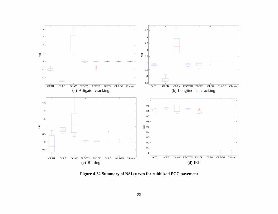
The main effects of all the input variables on all predicted distresses were investigated, as shown
in Figure 4-32. The distress and NSI plots for all of the inputs and distresses are presented in
Appendix B. The results show that overlay air voids has a significant impact on all the pavement
performance measures (NSI>1 for all cases). Overlay thickness, effective binder content, and
existing PCC modulus all have a significant impact on alligator cracking. In the case of rutting,
overlay effective binder content shows a significant impact. For IRI all design inputs except
overlay air voids show relatively lower contribution. It should be noted that box plot summarizes
a NSI curve for each design input range. In some cases if there is a rapid change in NSI due to a
specific input value, the point will be shown as an outlier in the box plot. Therefore, the
maximum value of NSI was used as the criteria for identifying a significant input variable.
Interactive effect of design inputs
Interaction between input variables for distress and NSI for this rehabilitation option are
presented in Appendix B. Figures B-96 to B-98 show the significant interactions for alligator
cracking and the corresponding NSI plots. The results in Figure B-96 show that lower overlay air
voids will reduce the impact of existing modulus on alligator cracking. For example, for low
overlay air voids and fair to high existing rubblized PCC modulus, the predicted cracking will be
negligible over the design life. On the other hand, for high overlay air voids depending on the
existing rubblized PCC modulus; the HMA layer may exhibit 0 to 50% alligator cracking over
the design life. Figure B-96 also shows that the rate of change in cracking w.r.t overlay air voids
will increase as the existing rubblized PCC modulus decreases. The maximum NSI for
interactions can be utilized to rank the interactions. The interactions are compared based on the
maximum NSI later in the summary of this section.

98
(a) Relative importance of design inputs for alligator cracking
(b) Relative importance of design inputs for longitudinal
cracking
(c) Relative importance of design inputs for rutting
(d) Relative importance of design inputs for IRI
Figure 4-31 Relative importance of design inputs for rubblized PCC pavement
OLTH OLEB OLAV EPCCTH EPCCE OLPG OLAGG Climate0
5
10
15
20
25
30
35
40
45
Rela
tiv
e I
mp
ort
an
ce
HMA over JPCP fractured - Alligator cracking
OLTH OLEB OLAV EPCCTH EPCCE OLPG OLAGG Climate0
5
10
15
20
25
30
Rela
tiv
e I
mp
ort
an
ce
HMA over JPCP fractured - Longitudinal cracking
OLTH OLEB OLAV EPCCTH EPCCE OLPG OLAGG Cliamte0
2
4
6
8
10
12
14
16
Rela
tiv
e I
mp
ort
an
ce
HMA over JPCP fractured - Rutting
OLTH OLEB OLAV EPCCTH EPCCE OLPG OLAGG Climate0
5
10
15
20
25
30
35
40
Rela
tiv
e I
mp
ort
an
ce
HMA over JPCP fractured - IRI
99
(a) Alligator cracking
(b) Longitudinal cracking
(c) Rutting
(d) IRI
Figure 4-32 Summary of NSI curves for rubblized PCC pavement
OLTH OLEB OLAV EPCCTH EPCCE OLPG OLAGG Climate
-2
-1
0
1
2
3
4
NS
I
OLTH OLEB OLAV EPCCTH EPCCE OLPG OLAGG Climate
-1.5
-1
-0.5
0
0.5
1
1.5
2
2.5
NS
I
OLTH OLEB OLAV EPCCTH EPCCE OLPG OLAGG Climate
-0.5
0
0.5
1
1.5
2
2.5
NS
I
OLTH OLEB OLAV EPCCTH EPCCE OLPG OLAGG Climate
0
0.1
0.2
0.3
0.4
0.5
0.6
0.7
0.8
0.9
1
NS
I
100
4.4.2.4. Unbonded PCC overlay
Relative importance of design inputs
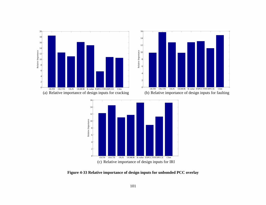
Figure 4-33 presents the relative importance of input variables for different pavement
performance measures. The results show that for cracking, overlay thickness, overlay MOR, and
subgrade modulus of reaction (k-value) have the most significant contributions. For faulting,
overlay CTE and climate are the major contributors. For IRI, overlay CTE, k-value, and climate
have important but somewhat similar contributions in predicted roughness.
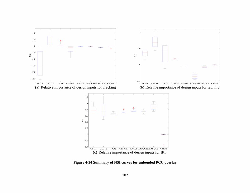
Main effect of design inputs
The summary of NSI plots for unbonded PCC overlay is presented in Figure 4-34. The main
effects of all the design inputs on all predicted distresses were investigated similarly to other
rehabilitation options and are presented in Appendix B. The results demonstrate that overlay
CTE has a significant impact on all pavement performance measures. For cracking, overlay
thickness has the highest effect followed by overlay MOR, CTE and joint spacing. Faulting and
IRI showed lower sensitivity to design inputs compared to cracking. However, overlay thickness
and existing PCC modulus show relatively large impact on IRI.
Interactive effect of design inputs
Figures B-140 to B-142 show the significant interactions for cracking and the corresponding NSI
interaction plots. Figure B-141 shows that higher overlay MOR will lower the impact of existing
PCC modulus on cracking. For example, for 900 psi overlay MOR, regardless of the existing
PCC modulus, the predicted cracking will be close to zero over the design life. On the other
hand, for low overlay MOR depending on the existing PCC modulus, the unbonded PCC overlay
will exhibit 20-40% cracking over the design life. Figure B-141 also shows that the rate of
change in cracking with respect to overlay MOR will decrease as the existing PCC modulus
increases. The interaction between existing modulus and overlay thickness has a significant
effect on cracking. The interaction between design inputs for faulting and IRI showed lower
effects. The maximum NSI for interactions can be used to rank the interactions.
101
(a) Relative importance of design inputs for cracking
(b) Relative importance of design inputs for faulting
(c) Relative importance of design inputs for IRI
Figure 4-33 Relative importance of design inputs for unbonded PCC overlay
OLTH OLCTE OLJS OLMOR K-value EXPCCTH EXPCCE Clim0
2
4
6
8
10
12
14
16
18
20
Rel
ativ
e Im
port
ance
OLTH OLCTE OLJS OLMOR K-value EXPCCTH EXPCCE Clim0
2
4
6
8
10
12
14
16
Rel
ativ
e Im
port
ance
OLTH OLCTE OLJS OLMOR K-value EXPCCTH EXPCCE Clim0
2
4
6
8
10
12
14
16
Rel
ativ
e Im
po
rtan
ce
102
(a) Relative importance of design inputs for cracking
(b) Relative importance of design inputs for faulting
(c) Relative importance of design inputs for IRI
Figure 4-34 Summary of NSI curves for unbonded PCC overlay
OLTH OLCTE OLJS OLMOR K-value EXPCCTH EXPCCE Climate
-25
-20
-15
-10
-5
0
5
10
NS
I
OLTH OLCTE OLJS OLMOR K-value EXPCCTH EXPCCE Climate
-0.5
0
0.5
1
NS
I
OLTH OLCTE OLJS OLMOR K-value EXPCCTH EXPCCE Climate-0.4
-0.2
0
0.2
0.4
0.6
0.8
1
1.2
NS
I
103
4.4.2.5. Summary Results
The four rehabilitation options were considered in GSA similarly to the preliminary and the
detailed sensitivity analyses. First, the relative contributions of the design inputs for various
pavement performance measures were identified and discussed. Second, the main effect of
design inputs for a base case was investigated. Finally the interactive effect of the design
inputs was studied for all pavement performance measures within each rehabilitation option.
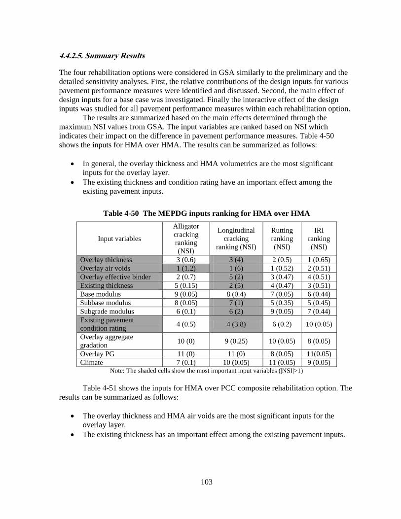
The results are summarized based on the main effects determined through the
maximum NSI values from GSA. The input variables are ranked based on NSI which
indicates their impact on the difference in pavement performance measures. Table 4-50
shows the inputs for HMA over HMA. The results can be summarized as follows:
In general, the overlay thickness and HMA volumetrics are the most significant
inputs for the overlay layer.
The existing thickness and condition rating have an important effect among the
existing pavement inputs.
Table 4-50 The MEPDG inputs ranking for HMA over HMA
Input variables
Alligator
cracking
ranking
(NSI)
Longitudinal
cracking
ranking (NSI)
Rutting
ranking
(NSI)
IRI
ranking
(NSI)
Overlay thickness 3 (0.6) 3 (4) 2 (0.5) 1 (0.65)
Overlay air voids 1 (1.2) 1 (6) 1 (0.52) 2 (0.51)
Overlay effective binder 2 (0.7) 5 (2) 3 (0.47) 4 (0.51)
Existing thickness 5 (0.15) 2 (5) 4 (0.47) 3 (0.51)
Base modulus 9 (0.05) 8 (0.4) 7 (0.05) 6 (0.44)
Subbase modulus 8 (0.05) 7 (1) 5 (0.35) 5 (0.45)
Subgrade modulus 6 (0.1) 6 (2) 9 (0.05) 7 (0.44)
Existing pavement
condition rating 4 (0.5) 4 (3.8) 6 (0.2) 10 (0.05)
Overlay aggregate
gradation 10 (0) 9 (0.25) 10 (0.05) 8 (0.05)
Overlay PG 11 (0) 11 (0) 8 (0.05) 11(0.05)
Climate 7 (0.1) 10 (0.05) 11 (0.05) 9 (0.05) Note: The shaded cells show the most important input variables (|NSI|>1)
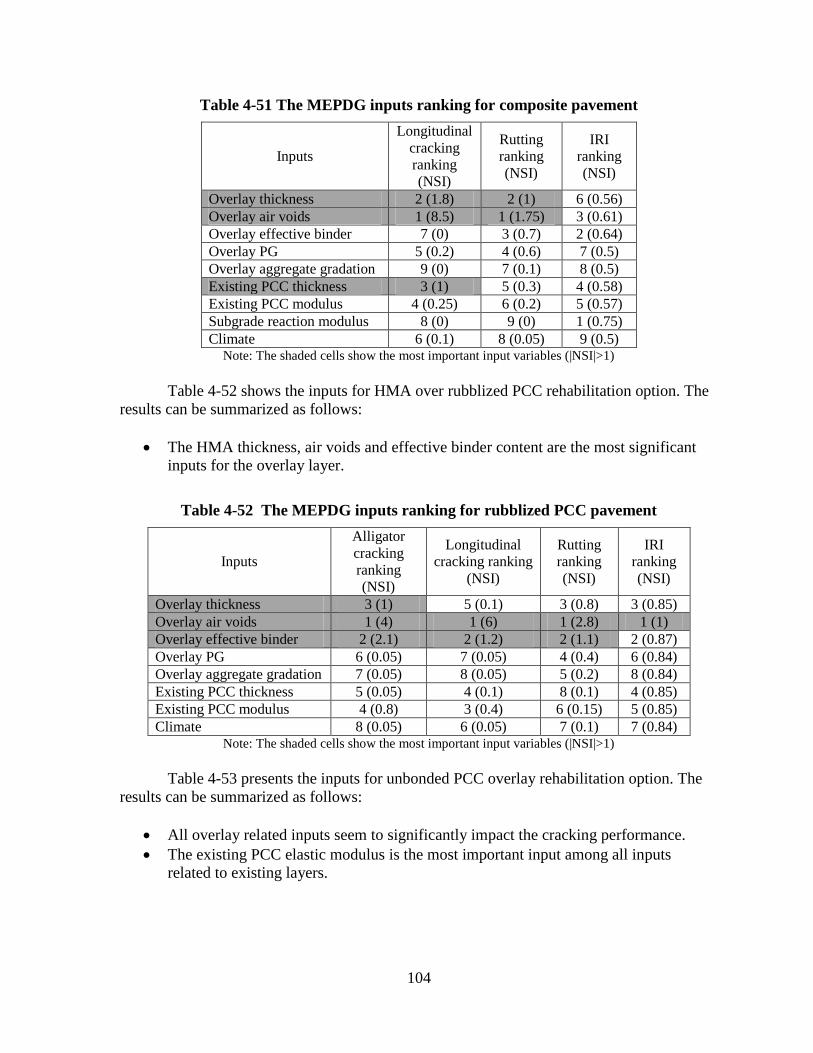
Table 4-51 shows the inputs for HMA over PCC composite rehabilitation option. The
results can be summarized as follows:
The overlay thickness and HMA air voids are the most significant inputs for the
overlay layer.
The existing thickness has an important effect among the existing pavement inputs.
104
Table 4-51 The MEPDG inputs ranking for composite pavement
Inputs
Longitudinal
cracking
ranking
(NSI)
Rutting
ranking
(NSI)
IRI
ranking
(NSI)
Overlay thickness 2 (1.8) 2 (1) 6 (0.56)
Overlay air voids 1 (8.5) 1 (1.75) 3 (0.61)
Overlay effective binder 7 (0) 3 (0.7) 2 (0.64)
Overlay PG 5 (0.2) 4 (0.6) 7 (0.5)
Overlay aggregate gradation 9 (0) 7 (0.1) 8 (0.5)
Existing PCC thickness 3 (1) 5 (0.3) 4 (0.58)
Existing PCC modulus 4 (0.25) 6 (0.2) 5 (0.57)
Subgrade reaction modulus 8 (0) 9 (0) 1 (0.75)
Climate 6 (0.1) 8 (0.05) 9 (0.5) Note: The shaded cells show the most important input variables (|NSI|>1)
Table 4-52 shows the inputs for HMA over rubblized PCC rehabilitation option. The
results can be summarized as follows:
The HMA thickness, air voids and effective binder content are the most significant
inputs for the overlay layer.
Table 4-52 The MEPDG inputs ranking for rubblized PCC pavement
Inputs
Alligator
cracking
ranking
(NSI)
Longitudinal
cracking ranking
(NSI)
Rutting
ranking
(NSI)
IRI
ranking
(NSI)
Overlay thickness 3 (1) 5 (0.1) 3 (0.8) 3 (0.85)
Overlay air voids 1 (4) 1 (6) 1 (2.8) 1 (1)
Overlay effective binder 2 (2.1) 2 (1.2) 2 (1.1) 2 (0.87)
Overlay PG 6 (0.05) 7 (0.05) 4 (0.4) 6 (0.84)
Overlay aggregate gradation 7 (0.05) 8 (0.05) 5 (0.2) 8 (0.84)
Existing PCC thickness 5 (0.05) 4 (0.1) 8 (0.1) 4 (0.85)
Existing PCC modulus 4 (0.8) 3 (0.4) 6 (0.15) 5 (0.85)
Climate 8 (0.05) 6 (0.05) 7 (0.1) 7 (0.84) Note: The shaded cells show the most important input variables (|NSI|>1)
Table 4-53 presents the inputs for unbonded PCC overlay rehabilitation option. The
results can be summarized as follows:
All overlay related inputs seem to significantly impact the cracking performance.
The existing PCC elastic modulus is the most important input among all inputs
related to existing layers.

105
Table 4-53 The MEPDG inputs ranking for unbonded PCC overlay
Design inputs
Cracking
ranking
(NSI)
Faulting
ranking
(NSI)
IRI
ranking
(NSI)
Overlay PCC thickness (inch) 1 (23) 4 (0.4) 2 (1.05)
Overlay PCC CTE (per °F x 10-6) 2 (12) 1 (1.1) 1 (1.2)
Overlay joint spacing (ft) 4 (5) 2 (0.55) 8 (0.75)
Overlay PCC MOR (psi) 3 (8) 5 (0.2) 5 (0.82)
Modulus of subgrade reaction (psi/in) 5 (0.5) 8 (0.1) 4 (0.88)
Existing PCC thickness (inch) 8 (0.1) 3 (0.45) 6 (0.81)
Existing PCC elastic modulus (psi) 6 (1) 7 (0.1) 3 (1.05)
Climate 7 (1) 6 (0.1) 7 (0.8) Note: The shaded cells show the most important input variables (|NSI|>1)
Tables 4-54 to 4-57 rank the interactions between input variations from overlay and
existing layer for all the rehabilitation options based on the maximum NSI. The results can be
summarized as follows:
The interaction between overlay air voids and existing pavement thickness seems to
be the most important in impacting all pavement performance measures among HMA
rehabilitation options. A higher air void in the overlay layers on a thin existing layer
seems to be the worst combination for predicted cracking.
The interaction between overlay thickness and existing PCC layer modulus seems to
have the most significant effect on unbonded PCC overlay performance. A thicker
overlay may hide the impact of weak existing PCC layer on pavement predicted
performance.
All the interactions studied here are practically and statistically significant. Therefore
all of them should be considered in the design and analysis.
Table 4-54 Interaction ranking for HMA over HMA
Interaction
Alligator
cracking
ranking
(NSI)
Longitudinal
cracking ranking
(NSI)
Rutting
ranking
(NSI)
IRI
ranking
(NSI)
Overlay air voids and
existing thickness 1 (0.8) 1 (15) 3 (0.3) 3 (0.1)
Overlay effective binder and
existing thickness 2 (0.5) 3 (7) 2 (0.3) 2 (0.1)
Overlay thickness and
existing thickness 3 (0.5) 2 (10) 1 (0.4) 1 (0.2)

106
Table 4-55 Interaction ranking for composite pavement
Interaction
Longitudinal
cracking
ranking (NSI)
Rutting
ranking
(NSI)
Overlay thickness and
existing thickness 2 (25) 2 (1.5)
Overlay air voids and
existing thickness 1 (44) 1 (1.7)
Table 4-56 Interaction ranking for rubblized PCC pavement
Interaction
Alligator
cracking
ranking (NSI)
Longitudinal
cracking ranking
(NSI)
Rutting
ranking
(NSI)
IRI
ranking
(NSI)
Overlay air voids and
existing thickness 1 (3.7) 1 (2.4) 2 (0.8) 2 (0.1)
Overlay effective binder and
existing thickness 2 (2.1) 2 (1.1) 1 (1) 1 (0.1)
Overlay thickness and
existing thickness 3 (0.8) 3 (0.5) 3 (0.8) 3 (0.1)
Table 4-57 Interaction ranking for unbonded PCC overlay
Interaction Cracking
ranking (NSI)
Faulting
ranking
(NSI)
IRI
ranking
(NSI)
Overlay thickness and
existing modulus 1 (28.5) 1 (0) 1 (1.5)
Overlay MOR and existing
thickness 3 (6) 2 (0) 3 (0.7)
Overlay MOR and existing
modulus 2 (14.5) 3 (0) 2 (0.7)
107
4.5 SATELLITE STUDIES
Several additional clarification studies were performed to evaluate the sensitivity of input
variables in the MEPDG/DARWin-ME. These investigations were important to understand
intricate details about the following topics:
1. Impact of HMA gradation on the predicted performance of flexible pavement
2. Effect of binder’s G* on predicted performance of HMA over HMA
3. Influence of unbound layers gradation on predicted performance of flexible and rigid
pavements
4.5.1 Effect of different HMA Gradations on Predicted Pavement
Performance
The main objective for this investigation was to evaluate the impact of HMA gradations
(level 3) on the predicted pavement performance based on the specification limits. Different
HMA gradations were obtained for the specific MDOT mixtures from Part 1 of the study.
The process for the selection of the HMA mixtures included the following steps:
a. Evaluate all HMA mixtures used in Part 1 of the project
b. Sort the mixtures by course type i.e., top, leveling, and base
c. Plot the aggregate gradation for each HMA mixture
d. Select a coarse, fine and intermediate gradation based on step c
e. Perform DARWin-ME analysis using the specific volumetric properties of the
selected HMA mixtures in step d
f. Compare the predicted pavement performance measures to evaluate the effect of
gradation.
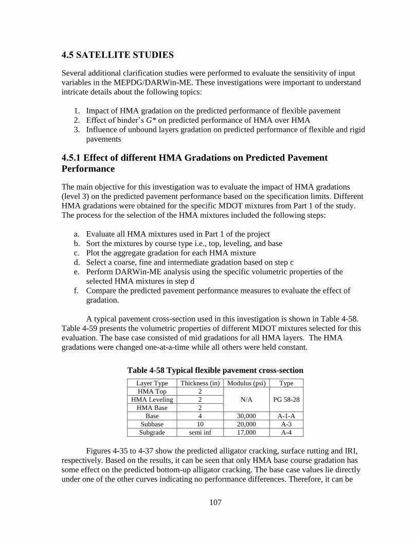
A typical pavement cross-section used in this investigation is shown in Table 4-58.
Table 4-59 presents the volumetric properties of different MDOT mixtures selected for this
evaluation. The base case consisted of mid gradations for all HMA layers. The HMA
gradations were changed one-at-a-time while all others were held constant.
Table 4-58 Typical flexible pavement cross-section
Layer Type Thickness (in) Modulus (psi) Type
HMA Top 2
N/A PG 58-28 HMA Leveling 2
HMA Base 2
Base 4 30,000 A-1-A
Subbase 10 20,000 A-3
Subgrade semi inf 17,000 A-4
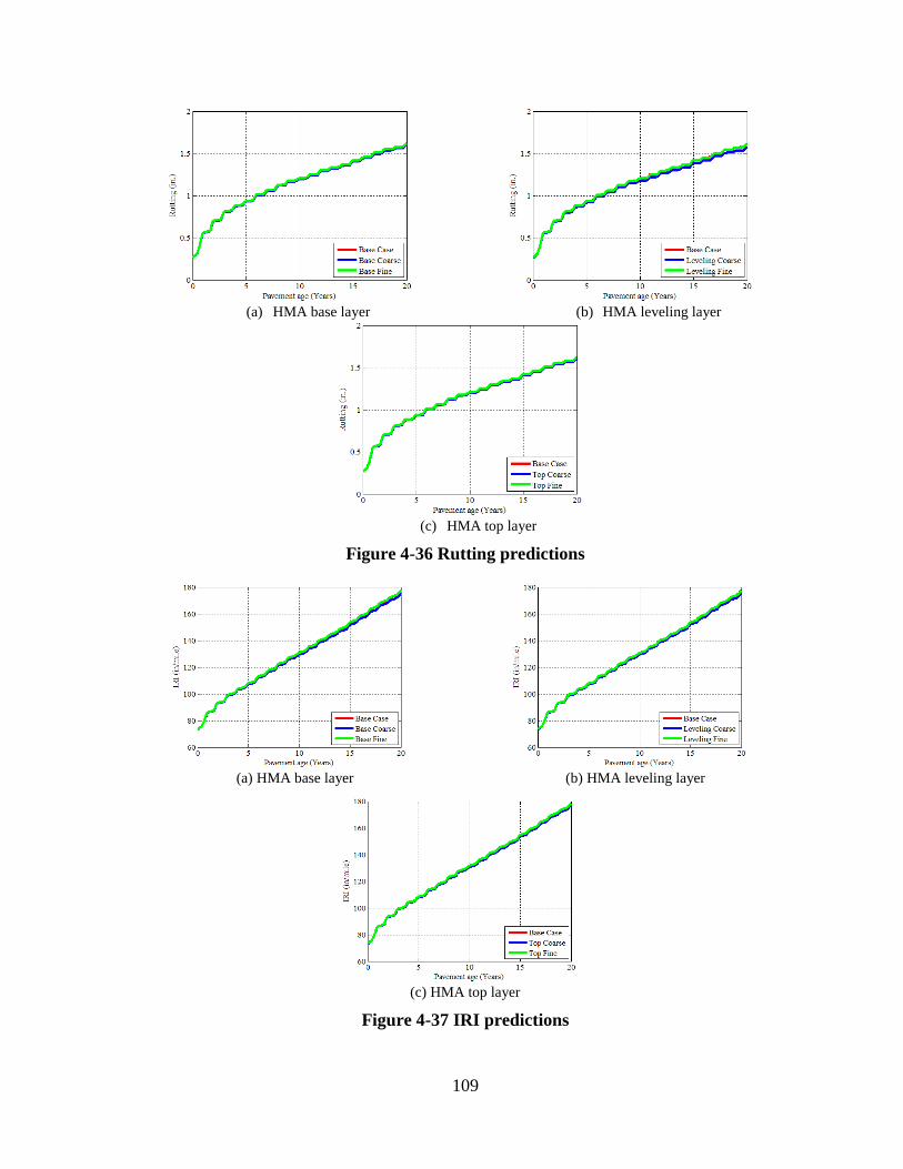
Figures 4-35 to 4-37 show the predicted alligator cracking, surface rutting and IRI,
respectively. Based on the results, it can be seen that only HMA base course gradation has
some effect on the predicted bottom-up alligator cracking. The base case values lie directly
under one of the other curves indicating no performance differences. Therefore, it can be

108
concluded that for level 3 inputs, HMA gradation doesn’t significantly impact the predicted
pavement performance. In addition, the average gradation from the specification limits can
be used for initial pavement design. However, it should be noted that these findings are valid
for the range of HMA gradations obtained in this study.
Table 4-59 Volumetric properties of the selected mixtures
Course type Gradation MDOT HMA mixture types
Mid (base case) Fine Coarse
Top
3/4" 100 100 100
3/8" 95.7 99.5 99.7
No. 4 80.1 76.2 84.1
No. 200 5.8 5.4 6
Eff AC 12.58 11.4 12.06
Leveling
3/4" 100 100 100
3/8" 87.6 89.9 87.1
No. 4 66.5 69.3 76.4
No. 200 5.7 5.6 5.3
Eff AC 10.62 10.9 10.58
Base
3/4" 100 100 99.9
3/8" 76.1 72.3 82.6
No. 4 56.9 47.3 65
No. 200 3.5 5 5.1
Eff AC 9.78 9.8 10.4
(a) HMA base layer
(b) HMA leveling layer
(c) HMA top layer
Figure 4-35 Alligator cracking predictions
109
(a) HMA base layer
(b) HMA leveling layer
(c) HMA top layer
Figure 4-36 Rutting predictions
(a) HMA base layer
(b) HMA leveling layer
(c) HMA top layer
Figure 4-37 IRI predictions

110
4.5.2 Impact of Binder G* Variations on Predicted Pavement Performance
In Part 1 of the study, several binders being used by MDOT were tested and characterized. It
was observed that multiple binders with similar PG can have significantly different
rheological behavior; i.e., master curves for dynamic shear modulus (G*). The main
objective of this investigation was to assess the variations in the MEPDG pavement
performance predictions due to multiple binders having the same PG but different G* master
curves. Figure 4-38 shows the G* master curves for two binders with the same PG grading
(PG 64-28). The two binders have different G* magnitude at different frequencies.
In order to evaluate the effect of G* on predicted performance of HMA over HMA, a
typical cross-section was selected. All inputs were held constant while G* data was used to
characterize the binder at level 1. Figure 4-39 shows the predicted pavement performance.
The results show that the effect of G* variation is only important for rutting prediction.
Therefore, it is recommended that G* master curve (level 1) should be used if available,
especially if rutting is a dominant distress. The variations in G* master curve could be
attributed to different binder sources for the same PG. However, it is anticipated that if a
binder from the same source is utilized for mix design at a specific location, the level 1 G*
master curve should not vary significantly. Therefore, an average can be used for multiple G*
master curves. Part 1 of this study addressed this issue in more detail.
Figure 4-38 The G* master curves for two binders with same PG
10
100
1,000
10,000
100,000
1,000,000
10,000,000
1.E-06 1.E-04 1.E-02 1.E+00 1.E+02
G*
(P
a)
Reduced Frequency, fr=f*a(T)
20B (NGBSU)
29B (NGBSU)

111
(a) Longitudinal cracking
(b) Alligator cracking
(c) Rutting
(d) IRI
Figure 4-39 The effect of G* variation on predicted HMA over HMA pavement
performance
4.5.3 Impact of Unbound Layer Gradations on Predicted Performance
The main objective of this investigation is to study the impact of aggregate base and subbase
gradations on the predicted performance. A sensitivity analysis was performed to study the
effects. Three gradations each were selected for base and subbase materials. The gradations
were selected for fine and coarse aggregates for each material type from the MDOT
specifications. In addition, the default gradation based on A-3 and A-1-a in the DARWin-ME
was considered for base and subbase materials, respectively. It should be noted that a
pavement structure can be designed based on several combinations of these materials with
different gradations. The design matrix for the sensitivity study is shown in Table 4-60. The
following procedure was used to select the coarse, and fine aggregate gradations:
1. Determine materials used for base and subbase from MDOT specifications
a. Base course – 22A, 21AA,
b. Subbase – Class II materials
2. Determine gradations from the MDOT specifications
a. Table 902-1 and 902-2 for base materials
b. Table 902-4 for subbase materials
3. Perform DARWin-ME analysis for both new JPCP and HMA pavements with coarse
(lower) and fine (upper) specification limits for base and subbase materials.
0
400
800
1200
1600
2000
2400
0 5 10 15 20
Lo
ng
itu
din
al cr
ack
ing
(ft
/mi)
Pavement age (years)
PG 64-28 (20B) PG 64-28 (29B) Threshold
0
4
8
12
16
20
24
0 5 10 15 20
All
iga
tor
cra
ckin
g (
%)
Pavement age (years)
PG 64-28 (20B) PG 64-28 (29B) Threshold
0
0.1
0.2
0.3
0.4
0.5
0.6
0 5 10 15 20
Ru
ttin
g (
in)
Pavement age (years)
PG 64-28 (20B) PG 64-28 (29B) Threshold
0
35
70
105
140
175
210
0 5 10 15 20IR
I (i
n/m
i)
Pavement age (years)
PG 64-28 (20B) PG 64-28 (29B) Threshold
112
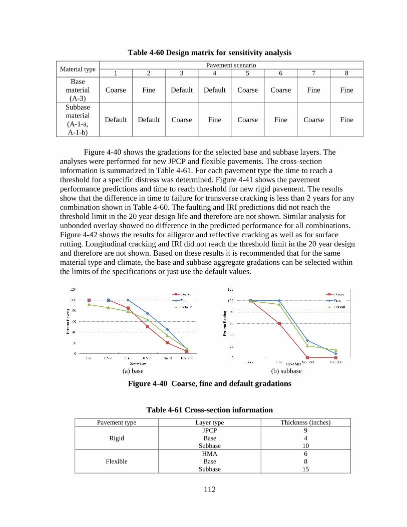
Table 4-60 Design matrix for sensitivity analysis
Material type Pavement scenario
1 2 3 4 5 6 7 8
Base
material
(A-3)
Coarse Fine Default Default Coarse Coarse Fine Fine
Subbase
material
(A-1-a,
A-1-b)
Default Default Coarse Fine Coarse Fine Coarse Fine
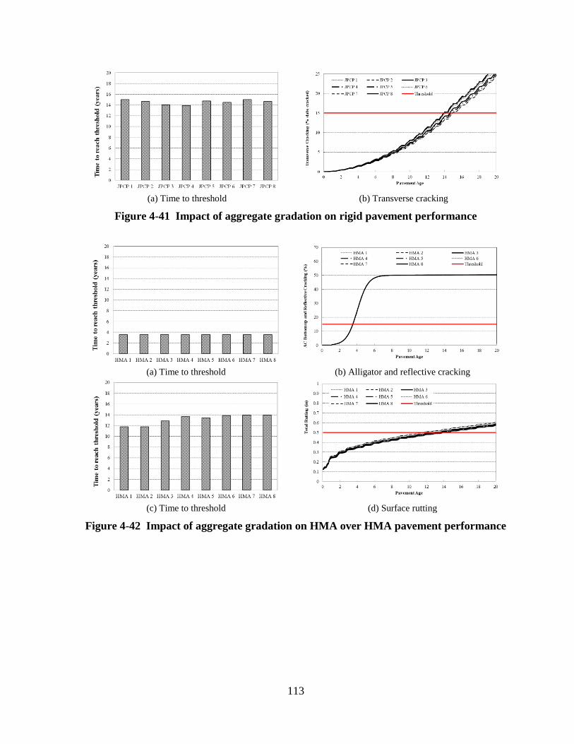
Figure 4-40 shows the gradations for the selected base and subbase layers. The
analyses were performed for new JPCP and flexible pavements. The cross-section
information is summarized in Table 4-61. For each pavement type the time to reach a
threshold for a specific distress was determined. Figure 4-41 shows the pavement
performance predictions and time to reach threshold for new rigid pavement. The results
show that the difference in time to failure for transverse cracking is less than 2 years for any
combination shown in Table 4-60. The faulting and IRI predictions did not reach the
threshold limit in the 20 year design life and therefore are not shown. Similar analysis for
unbonded overlay showed no difference in the predicted performance for all combinations.
Figure 4-42 shows the results for alligator and reflective cracking as well as for surface
rutting. Longitudinal cracking and IRI did not reach the threshold limit in the 20 year design
and therefore are not shown. Based on these results it is recommended that for the same
material type and climate, the base and subbase aggregate gradations can be selected within
the limits of the specifications or just use the default values.
(a) base
(b) subbase
Figure 4-40 Coarse, fine and default gradations
Table 4-61 Cross-section information
Pavement type Layer type Thickness (inches)
Rigid
JPCP
Base
Subbase
9
4
10
Flexible
HMA
Base
Subbase
6
8
15
113
(a) Time to threshold
(b) Transverse cracking
Figure 4-41 Impact of aggregate gradation on rigid pavement performance
(a) Time to threshold
(b) Alligator and reflective cracking
(c) Time to threshold
(d) Surface rutting
Figure 4-42 Impact of aggregate gradation on HMA over HMA pavement performance

114
CHAPTER 5 - VERIFICATION OF REHABILITATION DESIGN
5.1 INTRODUCTION
Validation of the MEPDG/DARWin-ME performance models is necessary to determine how
well the models predict measured pavement performance in the State of Michigan. The first
step in the verification process is to identify projects across different regions in the State
based on local pavement design and construction practices. The second step involves
extraction of the measured pavement performance data for each project from the MDOT
Pavement Management System (PMS) and Sensor (laser measured IRI, rutting and faulting)
database. The third step entails documentation of all input data related to pavement materials,
cross-section, traffic and climatic conditions for the identified projects. The accuracy of these
input data is important in determining the true predictability of the performance models in the
MEPDG/DARWin-ME. Finally, measured and predicted performances are compared for
each project to evaluate the existing performance models and to identify the local calibration
needs. It should be noted, that only DARWin-ME was used for the verification of the
rehabilitation models. In this chapter, the work related to the following tasks as outlined in
Chapter 1 is presented:
Task 2-4: Project identification and selection
Project selection criteria and matrix
Project information by rehabilitation option
Task 2-5: Verification of rehabilitation performance models
o Project performance
Available distresses in MDOT’s PMS and conversion to match
DARWin-ME
Project field performance
o Project Inputs for verification
o Verification results
Predicted vs. measured
Model accuracy
Need for local calibration
5.2 PROJECT IDENTIFICATION & SELECTION
In-service pavement projects were identified and selected to determine the validity of the
performance prediction models for Michigan. It should be noted that some identified
pavement projects may not be selected because they lack sufficient performance data or
adequate construction records. The project selection criteria, design matrix, and a summary
of the selected projects are discussed in the subsequent sections.

115
5.2.1 Project Selection Criteria and Design Matrix
MDOT identified and provided rehabilitation projects (unbonded, rubblized and composite
overlays) for the verification of the rehabilitation models. The MSU research team identified
HMA over HMA projects and MDOT provided the needed inputs. The HMA over HMA
pavement projects to be included in the study were selected based on the following criteria:
Site factors: The site factors will address the various regions in the state, climatic
zones and subgrade soil types.
Traffic: Three traffic levels were selected; level 1, less than 1000 AADTT, level 2,
1000 to 3000 AADTT; and level 3 more than 3000 AADTT. The three levels were
selected based on pavement class, trunk routes, US routes and Interstate routes.
Overlay thicknesses: The range of constructed overlay thicknesses.
Open to traffic date: The information is needed to determine the performance period.
As built cross-section: Includes details of the existing structure and the overlay.
Pre-overlay repairs performed on the existing pavement (such as partial and/or full
depth repairs, dowel bar retrofit)
Material properties of both the existing and the new structure
Table 5-1 summarizes the number of selected pavement projects based on the
selection criteria presented above. A total of 42 projects were selected representing various
rehabilitation options. It can be seen that each rehabilitation option contains more than 5
projects.
Table 5-1 Selection matrix displaying selected projects
Rehabilitation type Traffic
level*
Overlay
thickness
level*
Age (years)
Total <10 10 to 20 >20
Composite overlay
1 2 1 1
7 2 2 2 2
3 2 1
HMA over HMA 1
1 8
16 2 1 5
2 2 1 1
Rubblized overlay
1 2 4 2
11
3 2
2 2 1
3 2 1
3 1
Unbonded overlay 2
2 1
8 3 1
3 3 1 5
*Levels 1 2 3
Traffic (AADTT) <1000 1000-3000 >3000
Overlay thickness (in) <3 3-6 >6
116
5.2.2 Project Information by Rehabilitation Option
Pavement cross-section and material related information for each selected pavement project
are essential to generate the most representative project in the DARWin-ME. In addition, the
validity of the performance predictions using the software depends on how well the overlay
and existing pavement layers are defined. This section outlines the overlay, existing
pavement cross-section, and the geographical location information of the selected projects.
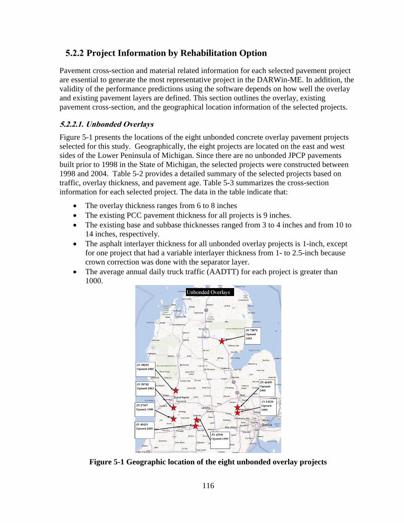
5.2.2.1. Unbonded Overlays
Figure 5-1 presents the locations of the eight unbonded concrete overlay pavement projects
selected for this study. Geographically, the eight projects are located on the east and west
sides of the Lower Peninsula of Michigan. Since there are no unbonded JPCP pavements
built prior to 1998 in the State of Michigan, the selected projects were constructed between
1998 and 2004. Table 5-2 provides a detailed summary of the selected projects based on
traffic, overlay thickness, and pavement age. Table 5-3 summarizes the cross-section
information for each selected project. The data in the table indicate that:
The overlay thickness ranges from 6 to 8 inches
The existing PCC pavement thickness for all projects is 9 inches.
The existing base and subbase thicknesses ranged from 3 to 4 inches and from 10 to
14 inches, respectively.
The asphalt interlayer thickness for all unbonded overlay projects is 1-inch, except
for one project that had a variable interlayer thickness from 1- to 2.5-inch because
crown correction was done with the separator layer.
The average annual daily truck traffic (AADTT) for each project is greater than
1000.
Figure 5-1 Geographic location of the eight unbonded overlay projects
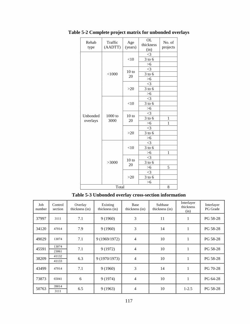
117
Table 5-2 Complete project matrix for unbonded overlays
Rehab
type
Traffic
(AADTT)
Age
(years)
OL
thickness
(in)
No. of
projects
Unbonded
overlays
<1000
<10
<3
3 to 6
>6
10 to
20
<3
3 to 6
>6
>20
<3
3 to 6
>6
1000 to
3000
<10
<3
3 to 6
>6
10 to
20
<3
3 to 6 1
>6 1
>20
<3
3 to 6
>6
>3000
<10
<3
3 to 6
>6 1
10 to
20
<3
3 to 6
>6 5
>20
<3
3 to 6
>6
Total 8
Table 5-3 Unbonded overlay cross-section information
Job
number
Control
section
Overlay
thickness (in)
Existing
thickness (in)
Base
thickness (in)
Subbase
thickness (in)
Interlayer
thickness
(in)
Interlayer
PG Grade
37997 3111 7.1 9 (1960) 3 11 1 PG 58-28
34120 47014 7.9 9 (1960) 3 14 1 PG 58-28
49029 13074 7.1 9 (1969/1972) 4 10 1 PG 58-28
45591 13074
7.1 9 (1972) 4 10 1 PG 58-28 23061
38209 41132
6.3 9 (1970/1973) 4 10 1 PG 58-28 41133
43499 47014 7.1 9 (1960) 3 14 1 PG 70-28
73873 65041 6 9 (1974) 4 10 1 PG 64-28
50763 39014
6.5 9 (1963) 4 10 1-2.5 PG 58-28 3111

118
5.2.2.2. Rubblized Overlays
Figure 5-2 shows the locations of the 11 selected rubblized projects. Geographically, all
projects are located in the Lower Peninsula of Michigan. The projects were constructed
between 1989 and 2000. The existing JRCP pavement was rubblized prior to applying an
HMA surface. Table 5-4 presents a detailed summary of the selected projects based on
traffic, overlay thickness, and pavement age. Table 5-5 lists the cross-section information for
each project. The data in the table indicate that:
The overlay thickness ranges from 4 to 9.5 inches.
The existing PCC pavement thicknesses ranged from 8 to 9 inches.
The existing base and subbase thicknesses range from 0 to 4 inches and from 0 to 18
inches, respectively.
Figure 5-2 Geographic location of the eleven rubblized overlay projects
N
O -
N
O -
N
O -
N
O -
N
O -
N
O -
N
O -
N
O -
N
O -
N
O -
N
O -
i s
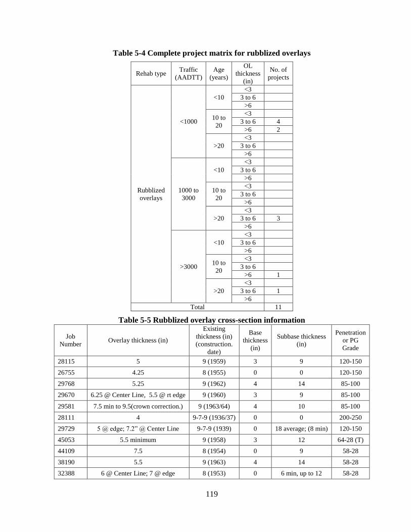
119
Table 5-4 Complete project matrix for rubblized overlays
Rehab type Traffic
(AADTT)
Age
(years)
OL
thickness
(in)
No. of
projects
Rubblized
overlays
<1000
<10
<3
3 to 6
>6
10 to
20
<3
3 to 6 4
>6 2
>20
<3
3 to 6
>6
1000 to
3000
<10
<3
3 to 6
>6
10 to
20
<3
3 to 6
>6
>20
<3
3 to 6 3
>6
>3000
<10
<3
3 to 6
>6
10 to
20
<3
3 to 6
>6 1
>20
<3
3 to 6 1
>6
Total 11
Table 5-5 Rubblized overlay cross-section information
Job
Number Overlay thickness (in)
Existing
thickness (in)
(construction.
date)
Base
thickness
(in)
Subbase thickness
(in)
Penetration
or PG
Grade
28115 5 9 (1959) 3 9 120-150
26755 4.25 8 (1955) 0 0 120-150
29768 5.25 9 (1962) 4 14 85-100
29670 6.25 @ Center Line, 5.5 @ rt edge 9 (1960) 3 9 85-100
29581 7.5 min to 9.5(crown correction.) 9 (1963/64) 4 10 85-100
28111 4 9-7-9 (1936/37) 0 0 200-250
29729 5 @ g ; 7.2” @ Center Line 9-7-9 (1939) 0 18 average; (8 min) 120-150
45053 5.5 minimum 9 (1958) 3 12 64-28 (T)
44109 7.5 8 (1954) 0 9 58-28
38190 5.5 9 (1963) 4 14 58-28
32388 6 @ Center Line; 7 @ edge 8 (1953) 0 6 min, up to 12 58-28
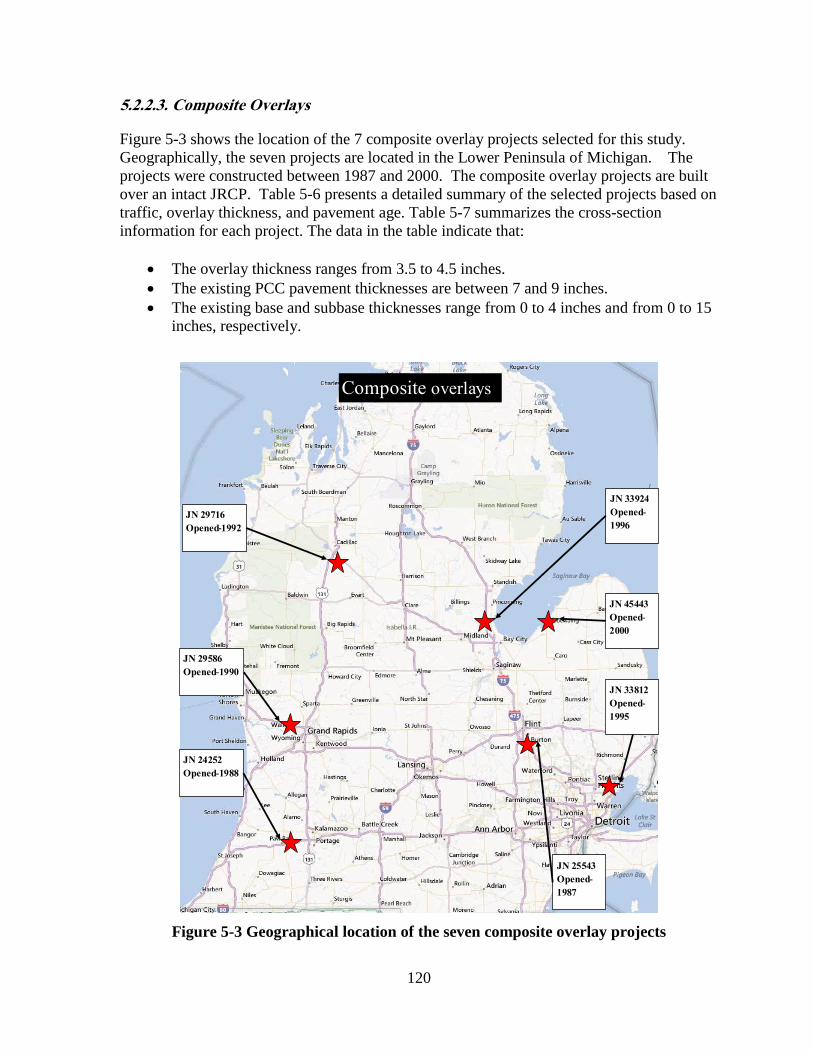
120
5.2.2.3. Composite Overlays
Figure 5-3 shows the location of the 7 composite overlay projects selected for this study.
Geographically, the seven projects are located in the Lower Peninsula of Michigan. The
projects were constructed between 1987 and 2000. The composite overlay projects are built
over an intact JRCP. Table 5-6 presents a detailed summary of the selected projects based on
traffic, overlay thickness, and pavement age. Table 5-7 summarizes the cross-section
information for each project. The data in the table indicate that:
The overlay thickness ranges from 3.5 to 4.5 inches.
The existing PCC pavement thicknesses are between 7 and 9 inches.
The existing base and subbase thicknesses range from 0 to 4 inches and from 0 to 15
inches, respectively.
Figure 5-3 Geographical location of the seven composite overlay projects
N
O -
N
O -
N
O -
N
O -
N
O -
N
O -
N
O -
C si s
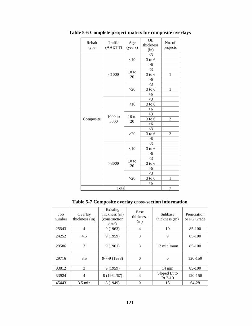
121
Table 5-6 Complete project matrix for composite overlays
Rehab
type
Traffic
(AADTT)
Age
(years)
OL
thickness
(in)
No. of
projects
Composite
<1000
<10
<3
3 to 6
>6
10 to
20
<3
3 to 6 1
>6
>20
<3
3 to 6 1
>6
1000 to
3000
<10
<3
3 to 6
>6
10 to
20
<3
3 to 6 2
>6
>20
<3
3 to 6 2
>6
>3000
<10
<3
3 to 6
>6
10 to
20
<3
3 to 6
>6
>20
<3
3 to 6 1
>6
Total 7
Table 5-7 Composite overlay cross-section information
Job
number
Overlay
thickness (in)
Existing
thickness (in)
(construction
date)
Base
thickness
(in)
Subbase
thickness (in)
Penetration
or PG Grade
25543 4 9 (1963) 4 10 85-100
24252 4.5 9 (1959) 3 9 85-100
29586 3 9 (1961) 3 12 minimum 85-100
29716 3.5 9-7-9 (1938) 0 0 120-150
33812 3 9 (1959) 3 14 min 85-100
33924 4 8 (1964/67) 4 Sloped Lt to
Rt 3-10 120-150
45443 3.5 min 8 (1949) 0 15 64-28

122
5.2.2.4. HMA over HMA
Figure 5-4 shows the location of 14 out of 15 HMA over HMA pavement projects selected
for this study. One of the projects did not meet all criteria and was excluded from the
verification study. Geographically, 14 projects are located in the Lower Peninsula and one
project in the Upper Peninsula of Michigan. In the Lower Peninsula, six projects are located
in the South West, five in the North West, and three projects are located in the Southern part
of the State. All projects were constructed between 1983 and 2005. The HMA over HMA
projects are built over existing flexible pavements. Table 5-8 presents a detailed summary of
the selected projects based on traffic, overlay thickness, and pavement age, while Table 5-9
summarizes the cross-section information. The data in the latter table indicate that:
The overlay thickness ranges from 2 to 3.5 inches.
The existing HMA pavement thicknesses range between 1.5 and 7.5 inches.
The existing base and subbase thicknesses range from 4 to 11 inches and from 0 to 28
inches respectively.
Figure 5-4 Geographical location of 14 HMA over HMA projects
N
O - M s
N
O -
N
O -
N
O -
N
O -
N
O -
N
O -
N
O -
N
O -
N
O -
N
O -
N
O - N
O -
N
O -
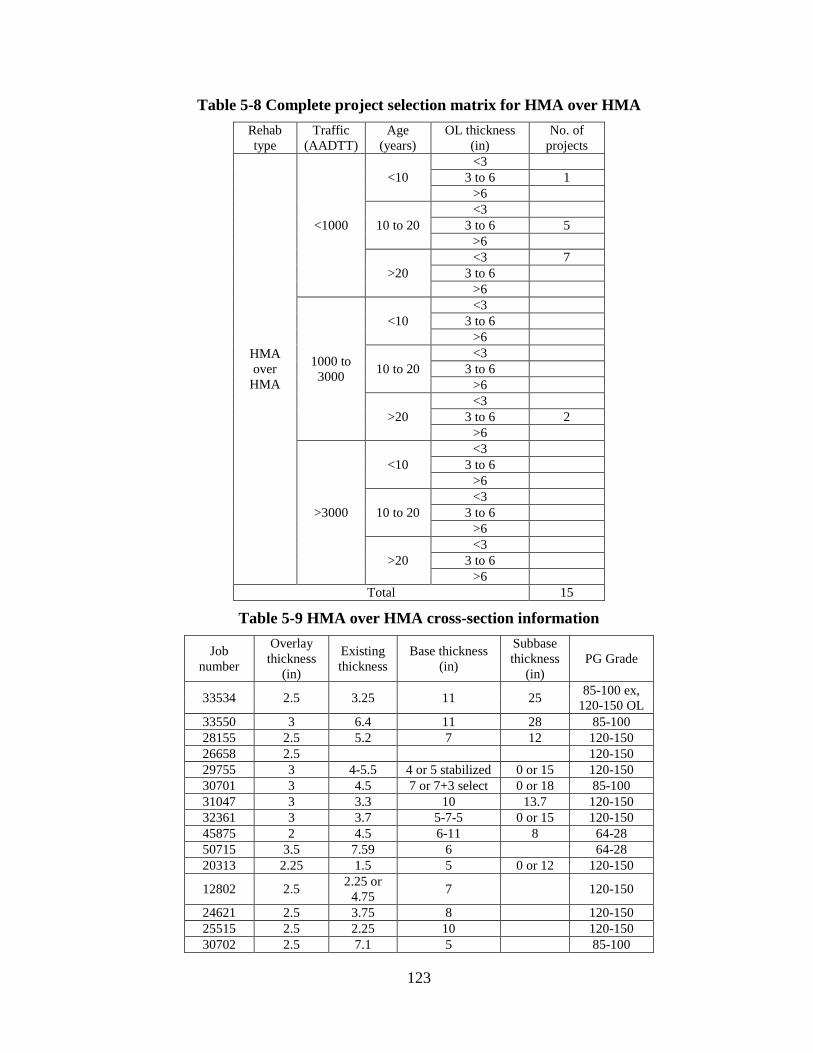
123
Table 5-8 Complete project selection matrix for HMA over HMA
Rehab
type
Traffic
(AADTT)
Age
(years)
OL thickness
(in)
No. of
projects
HMA
over
HMA
<1000
<10
<3
3 to 6 1
>6
10 to 20
<3
3 to 6 5
>6
>20
<3 7
3 to 6
>6
1000 to
3000
<10
<3
3 to 6
>6
10 to 20
<3
3 to 6
>6
>20
<3
3 to 6 2
>6
>3000
<10
<3
3 to 6
>6
10 to 20
<3
3 to 6
>6
>20
<3
3 to 6
>6
Total 15
Table 5-9 HMA over HMA cross-section information
Job
number
Overlay
thickness
(in)
Existing
thickness
Base thickness
(in)
Subbase
thickness
(in)
PG Grade
33534 2.5 3.25 11 25 85-100 ex,
120-150 OL
33550 3 6.4 11 28 85-100
28155 2.5 5.2 7 12 120-150
26658 2.5
120-150
29755 3 4-5.5 4 or 5 stabilized 0 or 15 120-150
30701 3 4.5 7 or 7+3 select 0 or 18 85-100
31047 3 3.3 10 13.7 120-150
32361 3 3.7 5-7-5 0 or 15 120-150
45875 2 4.5 6-11 8 64-28
50715 3.5 7.59 6
64-28
20313 2.25 1.5 5 0 or 12 120-150
12802 2.5 2.25 or
4.75 7
120-150
24621 2.5 3.75 8
120-150
25515 2.5 2.25 10
120-150
30702 2.5 7.1 5
85-100
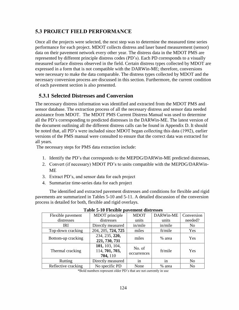
124
5.3 PROJECT FIELD PERFORMANCE
Once all the projects were selected, the next step was to determine the measured time series
performance for each project. MDOT collects distress and laser based measurement (sensor)
data on their pavement network every other year. The distress data in the MDOT PMS are
represented by different principle distress codes (PD’s). Each PD corresponds to a visually
measured surface distress observed in the field. Certain distress types collected by MDOT are
expressed in a form that is not compatible with the DARWin-ME; therefore, conversions
were necessary to make the data comparable. The distress types collected by MDOT and the
necessary conversion process are discussed in this section. Furthermore, the current condition
of each pavement section is also presented.
5.3.1 Selected Distresses and Conversion
The necessary distress information was identified and extracted from the MDOT PMS and
sensor database. The extraction process of all the necessary distress and sensor data needed
assistance from MDOT. The MDOT PMS Current Distress Manual was used to determine
all the PD’s corresponding to predicted distresses in the DARWin-ME. The latest version of
the document outlining all the different distress calls can be found in Appendix D. It should
be noted that, a PD’s w inc sinc MDOT g n c c ing his (1992), ier
versions of the PMS manual were consulted to ensure that the correct data was extracted for
all years.
The necessary steps for PMS data extraction include:
1. Identify the PD’s that corresponds to the MEPDG/DARWin-ME predicted distresses,
2. C n (if n c ss ) MDOT PD’s ni s compatible with the MEPDG/DARWin-
ME
3. Ex c PD’s, n s ns f ch j c
4. Summarize time-series data for each project
The identified and extracted pavement distresses and conditions for flexible and rigid
pavements are summarized in Tables 5-10 and 5-11. A detailed discussion of the conversion
process is detailed for both, flexible and rigid overlays.
Table 5-10 Flexible pavement distresses Flexible pavement
distresses
MDOT principle
distresses
MDOT
units
DARWin-ME
units
Conversion
needed?
IRI Directly measured in/mile in/mile No
Top-down cracking 204, 205, 724, 725 miles ft/mile Yes
Bottom-up cracking 234, 235, 220,
221, 730, 731 miles % area Yes
Thermal cracking
101, 103, 104,
114, 701, 703,
704, 110
No. of
occurrences ft/mile Yes
Rutting Directly measured in in No
Reflective cracking No specific PD None % area No *B n s s n PD’s h n c n in s

125
Table 5-11 Rigid pavement distresses
Rigid
pavement
distresses
MDOT principle
distresses
MDOT
units
DARWin-ME
units
Conversion
needed?
IRI Directly measured in/mile in/mile No
Faulting Directly measured in in No
Transverse
cracking 112, 113
No. of
occurrences
% slabs
cracked Yes
5.3.1.1. Distresses conversion for HMA designs
It should be noted that only the distress types predicted by the DARWin-ME were considered
for the verification exercise. The corresponding MDOT PD’s were determined and compared
to distress types predicted by the DARWin-ME to determine if any conversions were
necessary. The MDOT measured pavement distresses that are related to HMA overlays are
listed in Table 5-10. The conversion process (if necessary) for all distress types is as follows:
IRI: The IRI measurements in the MDOT sensor database are compatible to those in
DARWin-ME. Therefore, no conversion or adjustments was need and the data were used
directly.
Top-down cracking: Top-down cracking is defined as load related cracking in the wheel-path
(longitudinal cracking). The PD’s 204, 205, 724, and 725 are assumed to correspond to top
down cracking in the MDOT PMS database because those may not have developed an
indication of alligator cracking; however, these cracks could be bottom-up. The PD’s are
recorded in miles and needs conversion to feet/mile. Data from the wheel-paths were
summed into one value and divided by the total project length.
Bottom-up cracking: The bottom up cracking is defined as alligator cracking in the wheel-
path. The PD’s 234, 235, 220, 221, 730 and 731 match this requirement in the MDOT PMS
database. The PD’s have units of miles; however, to make those compatible with the
DARWin-ME alligator cracking units, conversion to percent total area is needed. This can be
achieved by using the following Equation (1):
Length of cracking width of wheelpaths
%Length of project Lane width
bottom upAC (1)
Thermal cracking: Thermal cracking corresponds to transverse cracking in flexible
pavements. The DARWin-ME predicts thermal cracking in feet/mile. The PD’s 101, 103,
104, 114, 701, 703 and 704 were utilized to extract transverse cracking in flexible and
rubblized pavements. For the composite pavement, PD’s 101, 110, 114 and 701 were used.
The transverse cracking is recorded as the number of occurrences. In order to convert
transverse cracking in feet/mile, the number of occurrences was multiplied by the lane width
for PD’s 101, 103 and 104. For the PDs 114 and 701, the number of occurrences was
multiplied by 3 feet because h s PD’s fin s “ s” (sh c cks) h less than
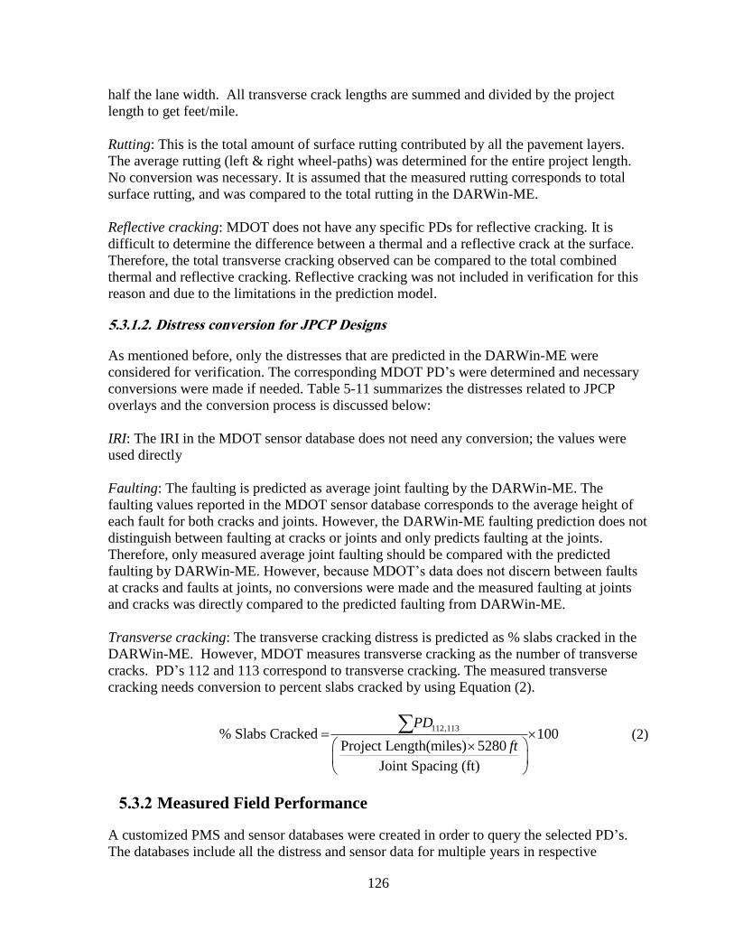
126
half the lane width. All transverse crack lengths are summed and divided by the project
length to get feet/mile.
Rutting: This is the total amount of surface rutting contributed by all the pavement layers.
The average rutting (left & right wheel-paths) was determined for the entire project length.
No conversion was necessary. It is assumed that the measured rutting corresponds to total
surface rutting, and was compared to the total rutting in the DARWin-ME.
Reflective cracking: MDOT does not have any specific PDs for reflective cracking. It is
difficult to determine the difference between a thermal and a reflective crack at the surface.
Therefore, the total transverse cracking observed can be compared to the total combined
thermal and reflective cracking. Reflective cracking was not included in verification for this
reason and due to the limitations in the prediction model.
5.3.1.2. Distress conversion for JPCP Designs
As mentioned before, only the distresses that are predicted in the DARWin-ME were
considered for verification. The corresponding MDOT PD’s were determined and necessary
conversions were made if needed. Table 5-11 summarizes the distresses related to JPCP
overlays and the conversion process is discussed below:
IRI: The IRI in the MDOT sensor database does not need any conversion; the values were
used directly
Faulting: The faulting is predicted as average joint faulting by the DARWin-ME. The
faulting values reported in the MDOT sensor database corresponds to the average height of
each fault for both cracks and joints. However, the DARWin-ME faulting prediction does not
distinguish between faulting at cracks or joints and only predicts faulting at the joints.
Therefore, only measured average joint faulting should be compared with the predicted
faulting by DARWin-ME. However, c s MDOT’s s n isc n w n f s
at cracks and faults at joints, no conversions were made and the measured faulting at joints
and cracks was directly compared to the predicted faulting from DARWin-ME.
Transverse cracking: The transverse cracking distress is predicted as % slabs cracked in the
DARWin-ME. However, MDOT measures transverse cracking as the number of transverse
cracks. PD’s 112 and 113 correspond to transverse cracking. The measured transverse
cracking needs conversion to percent slabs cracked by using Equation (2).
112, 113
% Slabs Cracked 100Project Length(miles) 5280
Joint Spacing (ft)
PD
ft
(2)
5.3.2 Measured Field Performance
A customized PMS and sensor databases were created in order to query the selected PD’s.
The databases include all the distress and sensor data for multiple years in respective
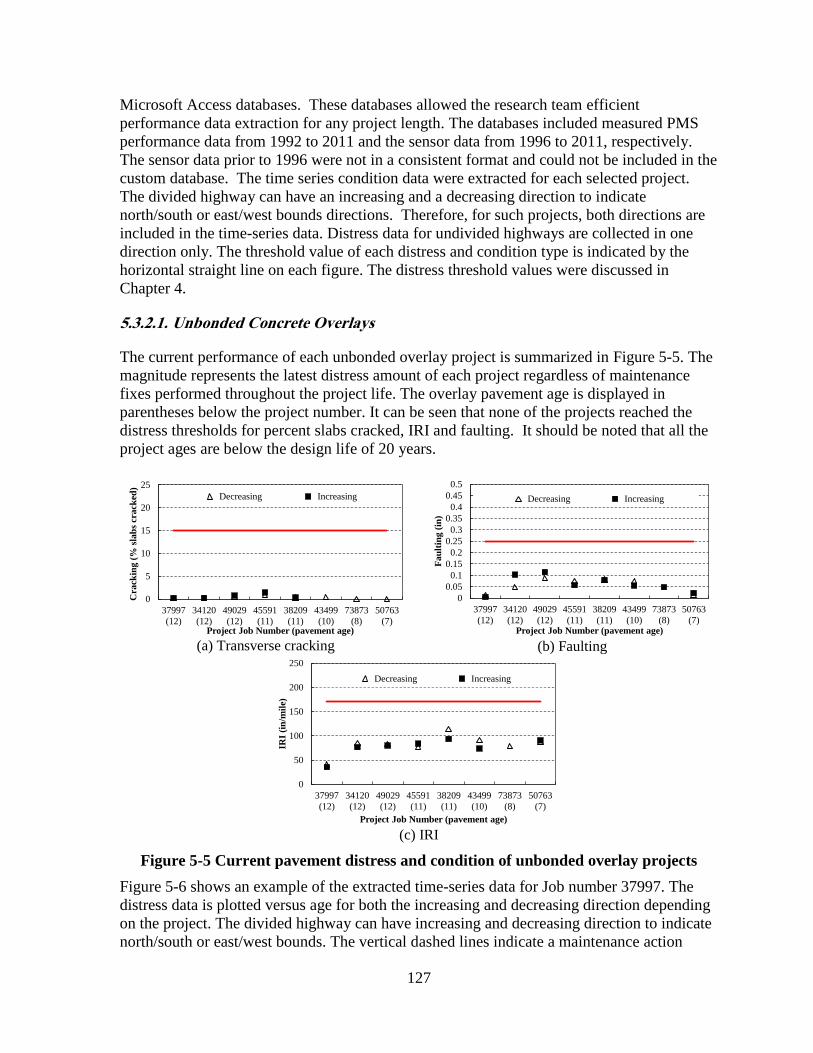
127
Microsoft Access databases. These databases allowed the research team efficient
performance data extraction for any project length. The databases included measured PMS
performance data from 1992 to 2011 and the sensor data from 1996 to 2011, respectively.
The sensor data prior to 1996 were not in a consistent format and could not be included in the
custom database. The time series condition data were extracted for each selected project.
The divided highway can have an increasing and a decreasing direction to indicate
north/south or east/west bounds directions. Therefore, for such projects, both directions are
included in the time-series data. Distress data for undivided highways are collected in one
direction only. The threshold value of each distress and condition type is indicated by the
horizontal straight line on each figure. The distress threshold values were discussed in
Chapter 4.
5.3.2.1. Unbonded Concrete Overlays
The current performance of each unbonded overlay project is summarized in Figure 5-5. The
magnitude represents the latest distress amount of each project regardless of maintenance
fixes performed throughout the project life. The overlay pavement age is displayed in
parentheses below the project number. It can be seen that none of the projects reached the
distress thresholds for percent slabs cracked, IRI and faulting. It should be noted that all the
project ages are below the design life of 20 years.
(a) Transverse cracking
(b) Faulting
(c) IRI
Figure 5-5 Current pavement distress and condition of unbonded overlay projects
Figure 5-6 shows an example of the extracted time-series data for Job number 37997. The
distress data is plotted versus age for both the increasing and decreasing direction depending
on the project. The divided highway can have increasing and decreasing direction to indicate
north/south or east/west bounds. The vertical dashed lines indicate a maintenance action
0
5
10
15
20
25
37997
(12)
34120
(12)
49029
(12)
45591
(11)
38209
(11)
43499
(10)
73873
(8)
50763
(7)
Cra
ckin
g (
% s
lab
s cr
ack
ed)
Project Job Number (pavement age)
Decreasing Increasing
0
0.05
0.1
0.15
0.2
0.25
0.3
0.35
0.4
0.45
0.5
37997
(12)
34120
(12)
49029
(12)
45591
(11)
38209
(11)
43499
(10)
73873
(8)
50763
(7)
Fau
ltin
g (
in)
Project Job Number (pavement age)
Decreasing Increasing
0
50
100
150
200
250
37997
(12)
34120
(12)
49029
(12)
45591
(11)
38209
(11)
43499
(10)
73873
(8)
50763
(7)
IRI
(in
/mil
e)
Project Job Number (pavement age)
Decreasing Increasing
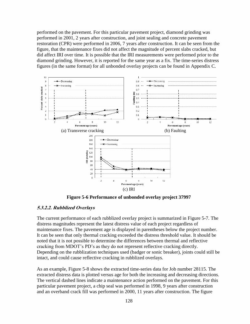
128
performed on the pavement. For this particular pavement project, diamond grinding was
performed in 2001, 2 years after construction, and joint sealing and concrete pavement
restoration (CPR) were performed in 2006, 7 years after construction. It can be seen from the
figure, that the maintenance fixes did not affect the magnitude of percent slabs cracked, but
did affect IRI over time. It is possible that the IRI measurements were performed prior to the
diamond grinding. However, it is reported for the same year as a fix. The time-series distress
figures (in the same format) for all unbonded overlay projects can be found in Appendix C.
(a) Transverse cracking
(b) Faulting
(c) IRI
Figure 5-6 Performance of unbonded overlay project 37997
5.3.2.2. Rubblized Overlays
The current performance of each rubblized overlay project is summarized in Figure 5-7. The
distress magnitudes represent the latest distress value of each project regardless of
maintenance fixes. The pavement age is displayed in parentheses below the project number.
It can be seen that only thermal cracking exceeded the distress threshold value. It should be
noted that it is not possible to determine the differences between thermal and reflective
c cking f MDOT’s PD’s s h n represent reflective cracking directly.
Depending on the rubblization techniques used (badger or sonic breaker), joints could still be
intact, and could cause reflective cracking in rubblized overlays.
As an example, Figure 5-8 shows the extracted time-series data for Job number 28115. The
extracted distress data is plotted versus age for both the increasing and decreasing directions.
The vertical dashed lines indicate a maintenance action performed on the pavement. For this
particular pavement project, a chip seal was performed in 1998, 9 years after construction
and an overband crack fill was performed in 2000, 11 years after construction. The figure
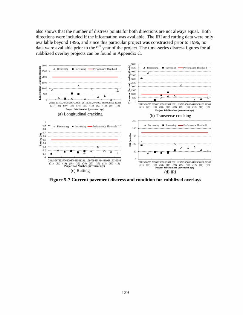
129
also shows that the number of distress points for both directions are not always equal. Both
directions were included if the information was available. The IRI and rutting data were only
available beyond 1996, and since this particular project was constructed prior to 1996, no
data were available prior to the 9th
year of the project. The time-series distress figures for all
rubblized overlay projects can be found in Appendix C.
(a) Longitudinal cracking
(b) Transverse cracking
(c) Rutting
(d) IRI
Figure 5-7 Current pavement distress and condition for rubblized overlays
0
500
1000
1500
2000
2500
3000
28115
(21)
26755
(21)
29768
(19)
29670
(18)
29581
(16)
28111
(20)
29729
(15)
45053
(12)
44109
(12)
38190
(10)
32388
(13)
Lo
ng
itu
din
al
Cra
ckin
g (
ft/m
ile)
Project Job Number (pavement age)
Decreasing Increasing Performance Threshold
0
500
1000
1500
2000
2500
3000
3500
4000
4500
5000
28115
(21)
26755
(21)
29768
(19)
29670
(18)
29581
(16)
28111
(20)
29729
(15)
45053
(12)
44109
(12)
38190
(10)
32388
(13)
Tra
nsv
erse
(th
erm
al)
cra
ckin
g (
ft/m
ile)
Project Job Number (pavement age)
Decreasing Increasing Performance Threshold
0
0.1
0.2
0.3
0.4
0.5
0.6
0.7
0.8
0.9
1
28115
(21)
26755
(21)
29768
(19)
29670
(18)
29581
(16)
28111
(20)
29729
(15)
45053
(12)
44109
(12)
38190
(10)
32388
(13)
Ru
ttin
g (
in)
Project Job Number (pavement age)
Decreasing Increasing Performance Threshold
0
50
100
150
200
250
28115
(21)
26755
(21)
29768
(19)
29670
(18)
29581
(16)
28111
(20)
29729
(15)
45053
(12)
44109
(12)
38190
(10)
32388
(13)
IRI
(in
/mil
e)
Project Job Number (pavement age)
Decreasing Increasing Performance Threshold

130
(a) Longitudinal cracking
(b) Transverse cracking
(c) Rutting
(d) IRI
Figure 5-8 Performance of rubblized overlay project 28115
5.3.2.3. Composite Overlays
The current performance of each composite overlay project is summarized in Figure 5-9. The
distress magnitudes represent the latest distress value of each project regardless of the
maintenance fixes. It can be seen that only thermal transverse cracking exceeded the distress
threshold. Similar to rubblized overlays, it is not possible to distinguish between reflective
c cking n h c cking in MDOT’s PMS s . I is ssi h s f h
thermal cracking is actually reflective cracking.
Figure 5-10 shows the extracted time-series data for Job number 29586. The extracted
distress data is plotted versus age for both the increasing and decreasing directions. The
vertical dashed lines indicate if a maintenance action has been performed on the pavement.
For this particular pavement project, a cold mill and resurfacing was performed in 1999, 9
years after construction. As mentioned for rubblized overlays, the missing IRI and rutting
data is due to the age of the project. The time-series distress figures for all composite overlay
projects can be found in Appendix C.
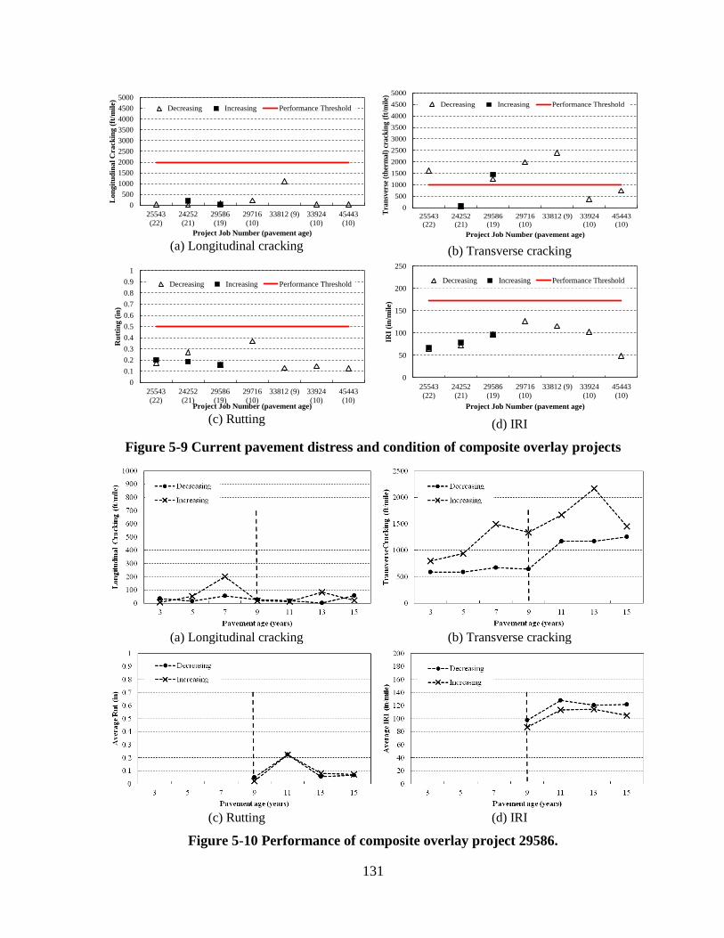
131
(a) Longitudinal cracking
(b) Transverse cracking
(c) Rutting
(d) IRI
Figure 5-9 Current pavement distress and condition of composite overlay projects
(a) Longitudinal cracking
(b) Transverse cracking
(c) Rutting
(d) IRI
Figure 5-10 Performance of composite overlay project 29586.
0
500
1000
1500
2000
2500
3000
3500
4000
4500
5000
25543
(22)
24252
(21)
29586
(19)
29716
(10)
33812 (9) 33924
(10)
45443
(10)
Lon
git
ud
inal
Cra
ckin
g (
ft/m
ile)
Project Job Number (pavement age)
Decreasing Increasing Performance Threshold
0
500
1000
1500
2000
2500
3000
3500
4000
4500
5000
25543
(22)
24252
(21)
29586
(19)
29716
(10)
33812 (9) 33924
(10)
45443
(10)
Tra
nsv
erse
(th
erm
al)
cra
ckin
g (
ft/m
ile)
Project Job Number (pavement age)
Decreasing Increasing Performance Threshold
0
0.1
0.2
0.3
0.4
0.5
0.6
0.7
0.8
0.9
1
25543
(22)
24252
(21)
29586
(19)
29716
(10)
33812 (9) 33924
(10)
45443
(10)
Ru
ttin
g (
in)
Project Job Number (pavement age)
Decreasing Increasing Performance Threshold
0
50
100
150
200
250
25543
(22)
24252
(21)
29586
(19)
29716
(10)
33812 (9) 33924
(10)
45443
(10)IR
I (i
n/m
ile)
Project Job Number (pavement age)
Decreasing Increasing Performance Threshold
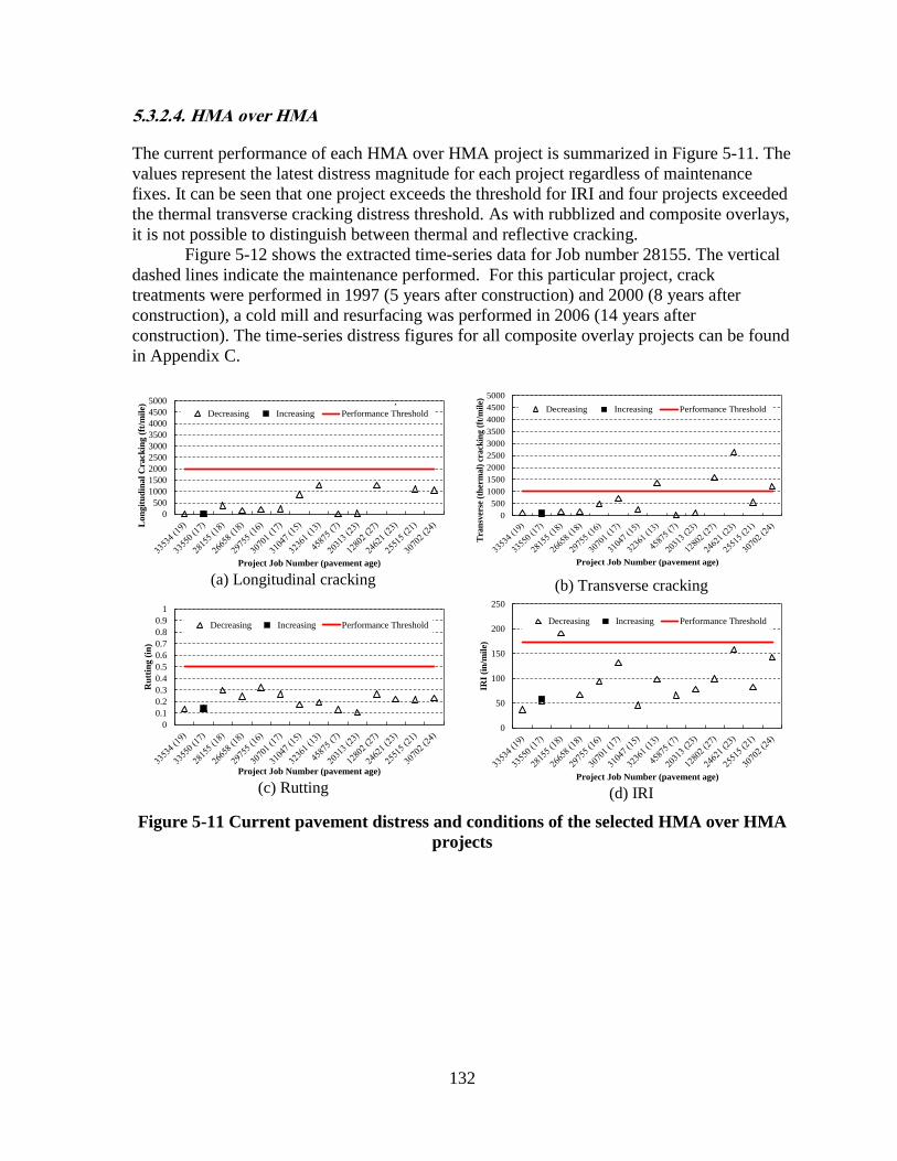
132
5.3.2.4. HMA over HMA
The current performance of each HMA over HMA project is summarized in Figure 5-11. The
values represent the latest distress magnitude for each project regardless of maintenance
fixes. It can be seen that one project exceeds the threshold for IRI and four projects exceeded
the thermal transverse cracking distress threshold. As with rubblized and composite overlays,
it is not possible to distinguish between thermal and reflective cracking.
Figure 5-12 shows the extracted time-series data for Job number 28155. The vertical
dashed lines indicate the maintenance performed. For this particular project, crack
treatments were performed in 1997 (5 years after construction) and 2000 (8 years after
construction), a cold mill and resurfacing was performed in 2006 (14 years after
construction). The time-series distress figures for all composite overlay projects can be found
in Appendix C.
(a) Longitudinal cracking
(b) Transverse cracking
(c) Rutting
(d) IRI
Figure 5-11 Current pavement distress and conditions of the selected HMA over HMA
projects
0
500
1000
1500
2000
2500
3000
3500
4000
4500
5000
Lon
git
ud
inal
Cra
ckin
g (
ft/m
ile)
Project Job Number (pavement age)
Decreasing Increasing Performance Threshold
0
500
1000
1500
2000
2500
3000
3500
4000
4500
5000
Tra
nsv
erse
(th
erm
al)
cra
ckin
g (
ft/m
ile)
Project Job Number (pavement age)
Decreasing Increasing Performance Threshold
0
0.1
0.2
0.3
0.4
0.5
0.6
0.7
0.8
0.9
1
Ru
ttin
g (
in)
Project Job Number (pavement age)
Decreasing Increasing Performance Threshold
0
50
100
150
200
250
IRI
(in
/mil
e)
Project Job Number (pavement age)
Decreasing Increasing Performance Threshold

133
(a) Longitudinal cracking
(b) Transverse cracking
(c) Rutting
(d) IRI
Figure 5-12 Performance of HMA over HMA project 28155.
The time-series plots presented here show the results of the extraction process from the
customized MDOT PMS and Sensor database. The magnitudes of the measured performance
data are critical for comparing the measured and predicted performance. The next section
discusses the process for identifying and collecting all the necessary input data to create the
most representative pavement project in DARWin-ME.
5.4 PROJECT INPUTS FOR VERIFICATION
The next step of the validation process consists of identifying and documenting input
variables for each selected project. The material, cross-section, climate, traffic, and existing
pavement condition information are essential to create the most representative project to be
analyzed in the DARWin-ME. The collection of required inputs needed extensive
collaboration with the MDOT RAP to ensure the appropriateness of the selected values. The
inputs for each project were obtained from MDOT historical records (project plans, material
records), the previous MDOT studies (Report numbers: RC-1516, RC-1531, and RC-1537),
and geographical location to select climate conditions.
5.4.1 Unbonded Overlays
The inputs for all unbonded overlay projects are summarized in Table 5-12. The inputs
needed to represent the as-constructed designs are discussed below.

134
Cross-section information
The pavement cross-section information was collected from the project design drawings
provided by MDOT. The cross-section for unbonded overlays consisted of thickness of
overlay layer, asphalt interlayer, existing PCC, base and subbase. Some projects did not have
all the necessary layer thicknesses; however, the missing pavement layer thicknesses were
determined after consultation with the RAP, or a typical design values for the time period of
project construction (new and existing) were recommended by MDOT.
Material related information
The material related information necessary for each pavement layer consisted of the
following:
Overlay PCC modulus of rupture (MOR)
Asphalt interlayer binder type and volumetric properties
Existing PCC elastic modulus
Base/subbase material type and resilient modulus
Subgrade soil type and resilient modulus
The overlay PCC modulus of rupture values were selected from the previous MDOT
study, RC-1516 because the study included typical values agreed upon by MDOT. The
asphalt interlayer binder type was determined from the mix design information extracted
from the MDOT historical records for each project. The existing PCC elastic modulus value
is the only way to characterize the condition of the underlying PCC pavement. The value of
3,000,000 psi was assumed because it is the upper limit suggested by the software as
discussed in Chapter 3. The base/subbase type and modulus values were also obtained from a
previous MDOT study (RC-1516) because the values were agreed upon by MDOT. The
subgrade soil type and resilient moduli values were obtained from a previous MDOT study
(RC-1531) which outlined the subgrade soil type and moduli values for the entire State of
Michigan.
Climate information
The climate information for each project was determined by their geographical location. The
DARWin-ME has a database for specific weather stations across the State of Michigan. The
closest weather station to the actual project was selected. If none of the pre-loaded weather
stations were located near the project, an interpolation was performed by selecting two or
more weather stations in the vicinity of the project.
Traffic information
The traffic information is essential and one of the most important inputs to analyze
pavements using the DARWin-ME. The annual average daily truck traffic (AADTT) was
determined from as-constructed project design drawings and by collaboration with the RAP.

135
When such information was not available, current traffic values were obtained from the
traffic maps specific to the project location which are available n MDOT’s w si
(<http://www.michigan.gov/mdot/0,4616,7-151-9622_11033-22141--,00.html>). The
AADTT values obtained from the website were back-casted to reflect the traffic at the time
of construction using a growth rate of two percent.
5.4.2 Rubblized Overlays
The inputs for all rubblized overlay projects are summarized in Table 5-13. The inputs
needed to represent the as-constructed projects as much as possible and are discussed below.
Cross-section information
The pavement cross-section information was collected from the project design drawings
provided by MDOT. The cross-section for rubblized overlays consisted of thickness of the
HMA overlay layer, existing fractured PCC layer, base and subbase. Some projects did not
have all the necessary layer thicknesses; however, the missing pavement layer thicknesses
were determined after consultation with the RAP, or typical design values for the time
period of project construction (new and existing) were recommended by MDOT.
Material related information
The material related information necessary for each pavement layer consisted of the
following:
Asphalt overlay binder type, mixture gradation, effective binder content, and air voids
Fractured PCC slab elastic modulus
Base/subbase material type and resilient modulus
Subgrade soil type and resilient modulus
The asphalt overlay layer properties were determined from the project job mix
formula information extracted from the historical data provided by MDOT. The HMA
volumetric properties were obtained from the job mix formula data sheets. The existing
rubblized PCC elastic modulus is the only way to classify the existing condition of the
rubblized layer. It was difficult to estimate this value; therefore, a value of 70,000 psi was
assumed based on discussions with MDOT. The base/subbase and subgrade soil types and
moduli values were obtained using the same procedure as for unbonded overlays.
Climate information
The climate information for each project was determined as discussed in the unbonded
overlay section.
Traffic information
The traffic information for each project was determined similar to unbonded overlay section.

136
5.4.3 Composite Overlays
The inputs for all composite overlay projects are summarized in Table 5-14. The inputs that
are needed to represent the as-constructed projects are discussed below.
Cross-section information
The pavement cross-section information was collected from the project design drawings
provided by MDOT. The cross-section for composite overlays consisted of thickness for the
overlay layer, existing intact PCC layer, base and subbase. Some projects did not have all the
necessary layer thicknesses; however, the missing pavement layer thicknesses were
determined after consultation with the RAP, or a typical design values for the time period of
project construction (new and existing) were recommended by MDOT.
Material related information
The material related information necessary to characterize each layer consisted of the
following:
Asphalt overlay binder type, mixture gradation, effective binder content, and air voids
Existing PCC MOR or elastic modulus
Base/subbase material type and resilient modulus
Subgrade soil type and resilient modulus
The asphalt overlay layer volumetric properties were determined from the project job
mix formulas obtained from the historical project data provided by MDOT. The existing
pavement is classified by the measured cracking, and how much of the measured cracking
was fixed during pre-overlay repairs. The PCC MOR was used to characterize the strength
of the existing layer similar to the unbonded overlay layer MOR. The base/subbase and
subgrade soil types and moduli values were obtained using the same procedure as for
unbonded overlays discussed previously.
Climate information
The climate information for each project was determined as discussed in the unbonded
overlay section.
Traffic information
The traffic information for each project was determined in a similar method as discussed in
the unbonded overlay section.
5.4.4 HMA over HMA
The inputs for all HMA over HMA projects are summarized in Table 5-15. The inputs
needed to represent the as-constructed projects are discussed below.

137
Cross-section information
The pavement cross-section information was collected from the project design drawings
provided by MDOT. The cross-section for HMA over HMA projects consisted of thickness
for the overlay layer, existing HMA layer, base and subbase. Some projects did not have all
the necessary layer thicknesses; however, the missing pavement layer thicknesses were
determined after consultation with the RAP, or a typical design values recommended by
MDOT were used.
Material related information
The material related information necessary to characterize each layer consisted of the
following:
Asphalt overlay binder type, mixture gradation, effective binder content, and air voids
Existing HMA pavement binder type, mixture gradation, effective binder content, and
air voids
Base/subbase material type and resilient modulus
Subgrade soil type and resilient modulus
The asphalt overlay layer properties were determined from the project historical data
provided by MDOT. The HMA volumetric properties of the overlay were obtained from the
job mix formula data sheets. The existing pavement was characterized by selecting the
condition rating of each project consisting of poor, fair and good conditions. Since the
existing condition is difficult to determine, the verification was performed for all three
conditions ratings. The HMA mixture properties for the existing pavement were obtained
from the job mix formula data sheets if available, otherwise, the values were assumed based
on projects in a similar climate, or by selecting properties from the MDOT specifications.
The specifications in effect during the time of original construction were used. The
base/subbase and subgrade soil types and moduli values were obtained using the same
procedure as for unbonded overlays discussed previously.
Climate information
The climate information for each project was determined as discussed in the unbonded
overlay section.
Traffic information
The traffic information for each project was determined in a similar method as discussed in
the unbonded overlay section.
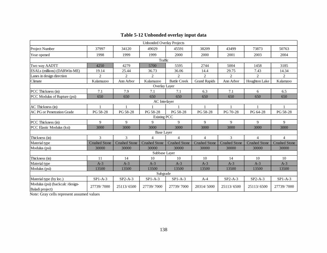
138
Table 5-12 Unbonded overlay input data
Note: Gray cells represent assumed values
Project Number 37997 34120 49029 45591 38209 43499 73873 50763
Year opened 1998 1999 1999 2000 2000 2001 2003 2004
Two way AADTT 4250 4279 5700 5595 2744 5004 1458 3185
ESALs (millions) (DARWin-ME) 19.14 25.44 36.73 36.06 14.4 29.75 7.43 14.34
Lanes in design direction 2 2 2 2 2 2 2 2
Climate Kalamazoo Ann Arbor Kalamazoo Battle Creek Grand Rapids Ann Arbor Houghton Lake Kalamzoo
PCC Thickness (in) 7.1 7.9 7.1 7.1 6.3 7.1 6 6.5
PCC Modulus of Rupture (psi) 650 650 650 650 650 650 650 650
AC Thickness (in) 1 1 1 1 1 1 1 1
AC PG or Penetration Grade PG 58-28 PG 58-28 PG 58-28 PG 58-28 PG 58-28 PG 70-28 PG 64-28 PG 58-28
PCC Thickness (in) 9 9 9 9 9 9 9 9
PCC Elastic Modulus (ksi) 3000 3000 3000 3000 3000 3000 3000 3000
Thickness (in) 3 3 4 4 4 3 4 4
Material type Crushed Stone Crushed Stone Crushed Stone Crushed Stone Crushed Stone Crushed Stone Crushed Stone Crushed Stone
Modulus (psi) 30000 30000 30000 30000 30000 30000 30000 30000
Thickness (in) 11 14 10 10 10 14 10 10
Material type A-3 A-3 A-3 A-3 A-3 A-3 A-3 A-3
Modulus (psi) 13500 13500 13500 13500 13500 13500 13500 13500
Material type (by loc.) SP1-A-3 SP2-A-3 SP1-A-3 SP1-A-3 A-4 SP2-A-3 SP2-A-3 SP1-A-3
Modulus (psi) (backcalc /design-
Baladi project)27739/ 7000 25113/ 6500 27739/ 7000 27739/ 7000 20314/ 5000 25113/ 6500 25113/ 6500 27739/ 7000
Subbase Layer
Subgrade
Unbonded Overlay Projects
Traffic
Overlay Layer
AC Interlayer
Existing PCC
Base Layer
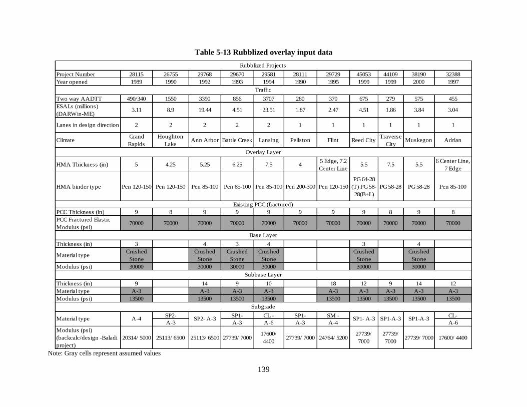
139
Table 5-13 Rubblized overlay input data
Note: Gray cells represent assumed values
Project Number 28115 26755 29768 29670 29581 28111 29729 45053 44109 38190 32388
Year opened 1989 1990 1992 1993 1994 1990 1995 1999 1999 2000 1997
Two way AADTT 490/340 1550 3390 856 3707 280 370 675 279 575 455
ESALs (millions)
(DARWin-ME)3.11 8.9 19.44 4.51 23.51 1.87 2.47 4.51 1.86 3.84 3.04
Lanes in design direction 2 2 2 2 2 1 1 1 1 1 1
ClimateGrand
Rapids
Houghton
LakeAnn Arbor Battle Creek Lansing Pellston Flint Reed City
Traverse
CityMuskegon Adrian
HMA Thickness (in) 5 4.25 5.25 6.25 7.5 45 Edge, 7.2
Center Line5.5 7.5 5.5
6 Center Line,
7 Edge
HMA binder type Pen 120-150 Pen 120-150 Pen 85-100 Pen 85-100 Pen 85-100 Pen 200-300 Pen 120-150
PG 64-28
(T) PG 58-
28(B+L)
PG 58-28 PG 58-28 Pen 85-100
PCC Thickness (in) 9 8 9 9 9 9 9 9 8 9 8
PCC Fractured Elastic
Modulus (psi)70000 70000 70000 70000 70000 70000 70000 70000 70000 70000 70000
Thickness (in) 3 4 3 4 3 4
Material typeCrushed
Stone
Crushed
Stone
Crushed
Stone
Crushed
Stone
Crushed
Stone
Crushed
Stone
Modulus (psi) 30000 30000 30000 30000 30000 30000
Thickness (in) 9 14 9 10 18 12 9 14 12
Material type A-3 A-3 A-3 A-3 A-3 A-3 A-3 A-3 A-3
Modulus (psi) 13500 13500 13500 13500 13500 13500 13500 13500 13500
SP2- SP1- CL - SP1- SM - CL-
A-3 A-3 A-6 A-3 A-4 A-6
Modulus (psi)
(backcalc/design -Baladi
project)
20314/ 5000 25113/ 6500 25113/ 6500 27739/ 700017600/
440027739/ 7000 24764/ 5200
27739/
7000
27739/
700027739/ 7000 17600/ 4400
Subbase Layer
Rubblized Projects
Traffic
Overlay Layer
Existing PCC (fractured)
Base Layer
Subgrade
Material type A-4 SP2- A-3 SP1- A-3 SP1-A-3 SP1-A-3
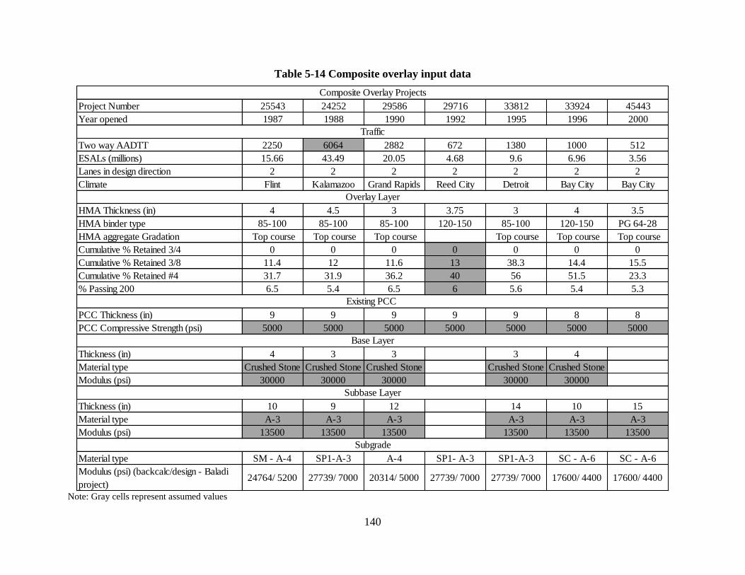
140
Table 5-14 Composite overlay input data
Note: Gray cells represent assumed values
Project Number 25543 24252 29586 29716 33812 33924 45443
Year opened 1987 1988 1990 1992 1995 1996 2000
Two way AADTT 2250 6064 2882 672 1380 1000 512
ESALs (millions) 15.66 43.49 20.05 4.68 9.6 6.96 3.56
Lanes in design direction 2 2 2 2 2 2 2
Climate Flint Kalamazoo Grand Rapids Reed City Detroit Bay City Bay City
HMA Thickness (in) 4 4.5 3 3.75 3 4 3.5
HMA binder type 85-100 85-100 85-100 120-150 85-100 120-150 PG 64-28
HMA aggregate Gradation Top course Top course Top course Top course Top course Top course
Cumulative % Retained 3/4 0 0 0 0 0 0 0
Cumulative % Retained 3/8 11.4 12 11.6 13 38.3 14.4 15.5
Cumulative % Retained #4 31.7 31.9 36.2 40 56 51.5 23.3
% Passing 200 6.5 5.4 6.5 6 5.6 5.4 5.3
PCC Thickness (in) 9 9 9 9 9 8 8
PCC Compressive Strength (psi) 5000 5000 5000 5000 5000 5000 5000
Thickness (in) 4 3 3 3 4
Material type Crushed Stone Crushed Stone Crushed Stone Crushed Stone Crushed Stone
Modulus (psi) 30000 30000 30000 30000 30000
Thickness (in) 10 9 12 14 10 15
Material type A-3 A-3 A-3 A-3 A-3 A-3
Modulus (psi) 13500 13500 13500 13500 13500 13500
Material type SM - A-4 SP1-A-3 A-4 SP1- A-3 SP1-A-3 SC - A-6 SC - A-6
Modulus (psi) (backcalc/design - Baladi
project)24764/ 5200 27739/ 7000 20314/ 5000 27739/ 7000 27739/ 7000 17600/ 4400 17600/ 4400
Subgrade
Composite Overlay Projects
Traffic
Overlay Layer
Existing PCC
Base Layer
Subbase Layer
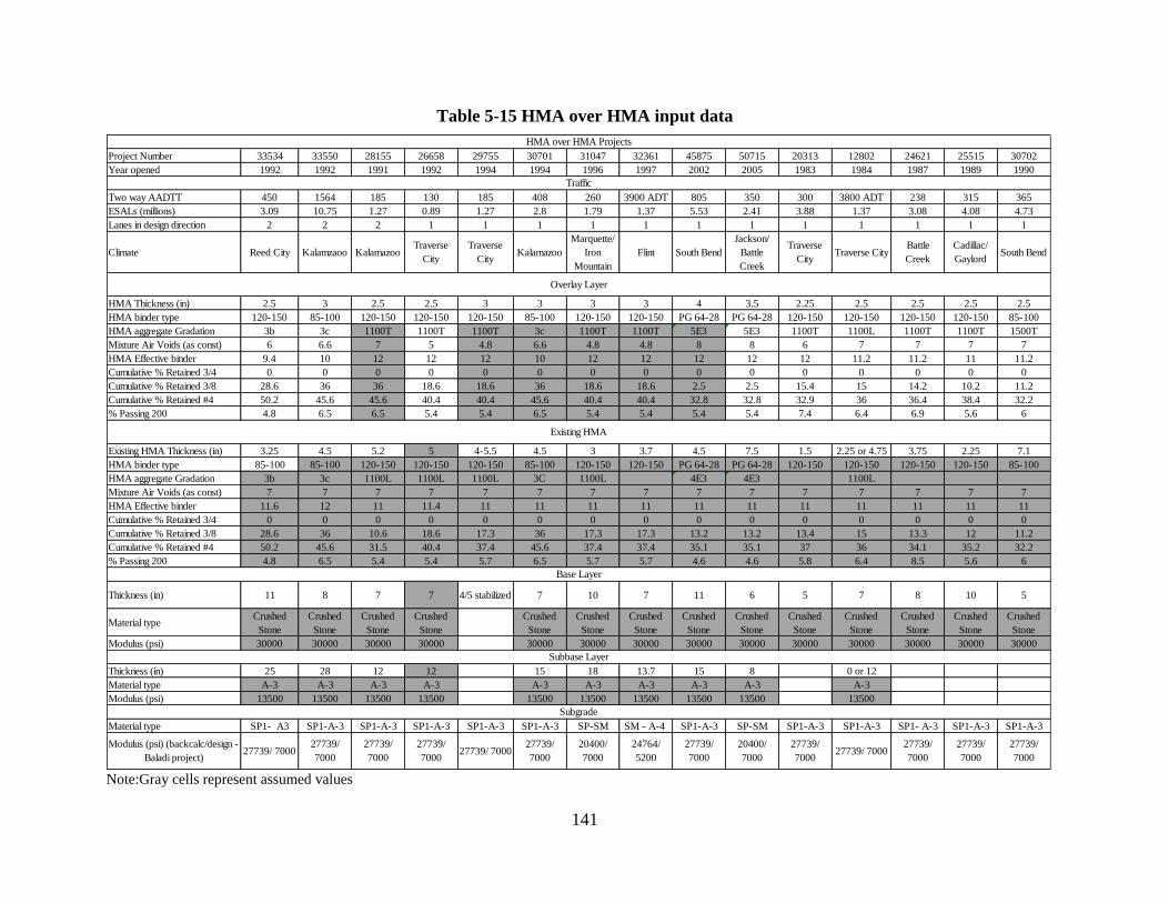
141
Table 5-15 HMA over HMA input data
Note:Gray cells represent assumed values
Project Number 33534 33550 28155 26658 29755 30701 31047 32361 45875 50715 20313 12802 24621 25515 30702
Year opened 1992 1992 1991 1992 1994 1994 1996 1997 2002 2005 1983 1984 1987 1989 1990
Two way AADTT 450 1564 185 130 185 408 260 3900 ADT 805 350 300 3800 ADT 238 315 365
ESALs (millions) 3.09 10.75 1.27 0.89 1.27 2.8 1.79 1.37 5.53 2.41 3.88 1.37 3.08 4.08 4.73
Lanes in design direction 2 2 2 1 1 1 1 1 1 1 1 1 1 1 1
Climate Reed City Kalamzaoo KalamazooTraverse
City
Traverse
CityKalamazoo
Marquette/
Iron
Mountain
Flint South Bend
Jackson/
Battle
Creek
Traverse
CityTraverse City
Battle
Creek
Cadillac/
GaylordSouth Bend
HMA Thickness (in) 2.5 3 2.5 2.5 3 3 3 3 4 3.5 2.25 2.5 2.5 2.5 2.5
HMA binder type 120-150 85-100 120-150 120-150 120-150 85-100 120-150 120-150 PG 64-28 PG 64-28 120-150 120-150 120-150 120-150 85-100
HMA aggregate Gradation 3b 3c 1100T 1100T 1100T 3c 1100T 1100T 5E3 5E3 1100T 1100L 1100T 1100T 1500T
Mixture Air Voids (as const) 6 6.6 7 5 4.8 6.6 4.8 4.8 8 8 6 7 7 7 7
HMA Effective binder 9.4 10 12 12 12 10 12 12 12 12 12 11.2 11.2 11 11.2
Cumulative % Retained 3/4 0 0 0 0 0 0 0 0 0 0 0 0 0 0 0
Cumulative % Retained 3/8 28.6 36 36 18.6 18.6 36 18.6 18.6 2.5 2.5 15.4 15 14.2 10.2 11.2
Cumulative % Retained #4 50.2 45.6 45.6 40.4 40.4 45.6 40.4 40.4 32.8 32.8 32.9 36 36.4 38.4 32.2
% Passing 200 4.8 6.5 6.5 5.4 5.4 6.5 5.4 5.4 5.4 5.4 7.4 6.4 6.9 5.6 6
Existing HMA Thickness (in) 3.25 4.5 5.2 5 4-5.5 4.5 3 3.7 4.5 7.5 1.5 2.25 or 4.75 3.75 2.25 7.1
HMA binder type 85-100 85-100 120-150 120-150 120-150 85-100 120-150 120-150 PG 64-28 PG 64-28 120-150 120-150 120-150 120-150 85-100
HMA aggregate Gradation 3b 3c 1100L 1100L 1100L 3C 1100L 4E3 4E3 1100L
Mixture Air Voids (as const) 7 7 7 7 7 7 7 7 7 7 7 7 7 7 7
HMA Effective binder 11.6 12 11 11.4 11 11 11 11 11 11 11 11 11 11 11
Cumulative % Retained 3/4 0 0 0 0 0 0 0 0 0 0 0 0 0 0 0
Cumulative % Retained 3/8 28.6 36 10.6 18.6 17.3 36 17.3 17.3 13.2 13.2 13.4 15 13.3 12 11.2
Cumulative % Retained #4 50.2 45.6 31.5 40.4 37.4 45.6 37.4 37.4 35.1 35.1 37 36 34.1 35.2 32.2
% Passing 200 4.8 6.5 5.4 5.4 5.7 6.5 5.7 5.7 4.6 4.6 5.8 6.4 8.5 5.6 6
Thickness (in) 11 8 7 7 4/5 stabilized 7 10 7 11 6 5 7 8 10 5
Material typeCrushed
Stone
Crushed
Stone
Crushed
Stone
Crushed
Stone
Crushed
Stone
Crushed
Stone
Crushed
Stone
Crushed
Stone
Crushed
Stone
Crushed
Stone
Crushed
Stone
Crushed
Stone
Crushed
Stone
Crushed
Stone
Modulus (psi) 30000 30000 30000 30000 30000 30000 30000 30000 30000 30000 30000 30000 30000 30000
Thickness (in) 25 28 12 12 15 18 13.7 15 8 0 or 12
Material type A-3 A-3 A-3 A-3 A-3 A-3 A-3 A-3 A-3 A-3
Modulus (psi) 13500 13500 13500 13500 13500 13500 13500 13500 13500 13500
Material type SP1- A3 SP1-A-3 SP1-A-3 SP1-A-3 SP1-A-3 SP1-A-3 SP-SM SM - A-4 SP1-A-3 SP-SM SP1-A-3 SP1-A-3 SP1- A-3 SP1-A-3 SP1-A-3
Subbase Layer
HMA over HMA Projects
Traffic
Overlay Layer
Existing HMA
Base Layer
Subgrade
Modulus (psi) (backcalc/design -
Baladi project)27739/ 7000
27739/
7000
27739/
7000
27739/
700027739/ 7000
27739/
7000
20400/
7000
24764/
5200
27739/
7000
27739/
7000
20400/
7000
27739/
700027739/ 7000
27739/
7000
27739/
7000
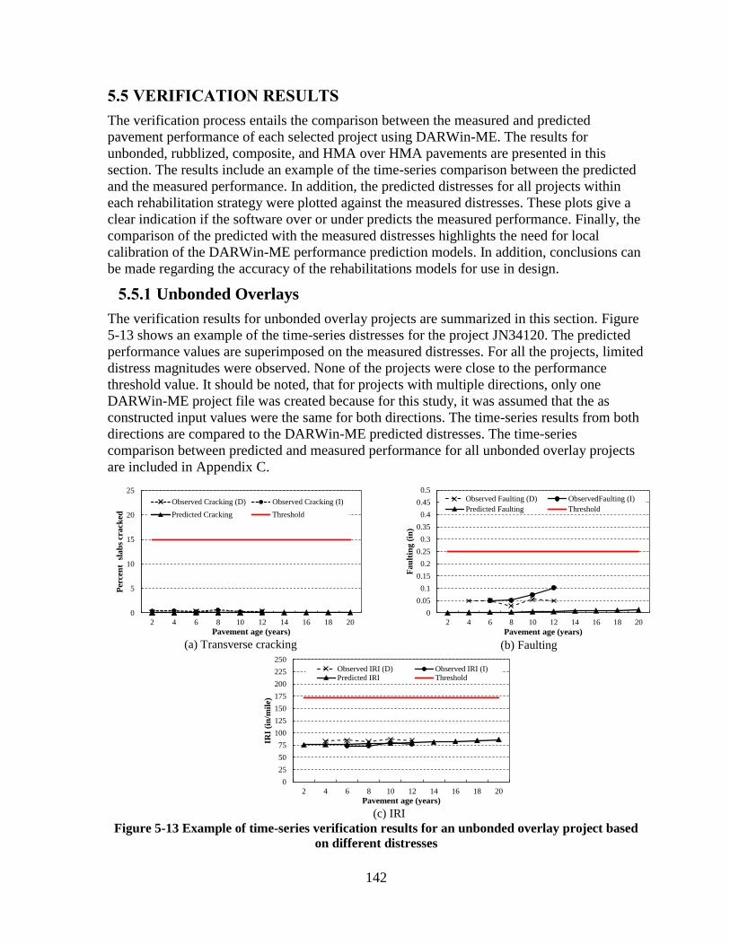
142
5.5 VERIFICATION RESULTS
The verification process entails the comparison between the measured and predicted
pavement performance of each selected project using DARWin-ME. The results for
unbonded, rubblized, composite, and HMA over HMA pavements are presented in this
section. The results include an example of the time-series comparison between the predicted
and the measured performance. In addition, the predicted distresses for all projects within
each rehabilitation strategy were plotted against the measured distresses. These plots give a
clear indication if the software over or under predicts the measured performance. Finally, the
comparison of the predicted with the measured distresses highlights the need for local
calibration of the DARWin-ME performance prediction models. In addition, conclusions can
be made regarding the accuracy of the rehabilitations models for use in design.
5.5.1 Unbonded Overlays
The verification results for unbonded overlay projects are summarized in this section. Figure
5-13 shows an example of the time-series distresses for the project JN34120. The predicted
performance values are superimposed on the measured distresses. For all the projects, limited
distress magnitudes were observed. None of the projects were close to the performance
threshold value. It should be noted, that for projects with multiple directions, only one
DARWin-ME project file was created because for this study, it was assumed that the as
constructed input values were the same for both directions. The time-series results from both
directions are compared to the DARWin-ME predicted distresses. The time-series
comparison between predicted and measured performance for all unbonded overlay projects
are included in Appendix C.
(a) Transverse cracking
(b) Faulting
(c) IRI
Figure 5-13 Example of time-series verification results for an unbonded overlay project based
on different distresses
0
5
10
15
20
25
2 4 6 8 10 12 14 16 18 20
Per
cen
t s
lab
s cr
ack
ed
Pavement age (years)
Observed Cracking (D) Observed Cracking (I)
Predicted Cracking Threshold
0
0.05
0.1
0.15
0.2
0.25
0.3
0.35
0.4
0.45
0.5
2 4 6 8 10 12 14 16 18 20
Fa
ult
ing
(in
)
Pavement age (years)
Observed Faulting (D) ObservedFaulting (I)
Predicted Faulting Threshold
0
25
50
75
100
125
150
175
200
225
250
2 4 6 8 10 12 14 16 18 20
IRI
(in
/mil
e)
Pavement age (years)
Observed IRI (D) Observed IRI (I)Predicted IRI Threshold

143
Figure 5-14(a) shows that DARWin-ME under predicts the measured cracking for the
unbonded overlay projects. The faulting model also under predicts the measured faulting as
shown in Figure 5-14(b). The measured and predicted faulting values are minimal and do not
reach the threshold limit. It is expected that minimal faulting should be predicted in
DARWin-ME because dowels (1.25 inch in diameter) were included in the design for load
transfer at the joint. The IRI predicted values (Figure 5-14c) are closer to the measured
performance. Based on these results, calibration of all the performance models for unbonded
overlay is necessary to improve the accuracy of DARWin-ME for the Michigan conditions.
(a) Transverse cracking
(b) Faulting
(c) IRI
Figure 5-14 Predicted vs. measured results for all unbonded overlay projects.
5.5.2 Rubblized Overlays
The verification results for rubblized overlay projects are summarized in this section. The
verification was performed using two different subgrade moduli (see the back-calculated and
design MR values in Table 2-9 which are from MDOT Report Number RC-1531). The back-
calculated values were not determined in this study. The subgrade modulus has significant
effect on rutting performance. Figure 5-15 shows an example of the time-series comparison
between predicted and measured performance for the project JN44109. Figure 5-16
summarizes the predicted vs. measured performance for all rubblized projects using the back-
calculated subgrade moduli. Figure 5-17 illustrates the same results with the adjusted
recommended design subgrade modulus values. The time-series comparison between
predicted and measured performance for all rubblized overlay projects are included in
Appendix C
0
5
10
15
20
25
30
0 5 10 15 20 25 30
Pre
dic
ted
Cra
ckin
g (
% s
lab
s cr
ack
ed)
Measured Cracking (% slabs cracked)
0
0.1
0.2
0.3
0.4
0.5
0 0.1 0.2 0.3 0.4 0.5
Pred
icte
d F
au
ltin
g (
in)
Measured Faulting (in)
0
50
100
150
200
250
0 50 100 150 200 250
Pre
dic
ted
IR
I (i
n/m
ile)
Measured IRI (in/mile)

144
The results in Figure 5-16 and Figure 5-17 illustrate that the predictions are not close to the
line of equality. It can be concluded that the design software under-predicts longitudinal
cracking for most of the pavement sections. The thermal transverse cracking model under-
predicts the measured performance. The minimal amount of thermal transverse cracking
predicted by the software could be due to appropriate binder selection for a specific climate.
However, this is not observed in the field as each selected project has significant amounts of
measured transverse cracking. It should be noted that several of the selected projects were
constructed prior to Superpave binder specification were adopted for design. Thus, climatic
considerations were not taken into account during binder selection. It is observed that the
software over predicts the measured distresses for both rutting and IRI. The design value
subgrade MR over predicted rutting more than the backcalculated MR. Therefore, calibration
of all the performance models is necessary to improve the accuracy of DARWin-ME for the
Michigan conditions. Based on the results, it is also recommended to use backcalculation to
determine the subgrade soil condition.
(a) Longitudinal cracking
(b) Transverse cracking
(c) Rutting
(d) IRI
Figure 5-15 Example of time-series verification results for a rubblized overlay project
based on different distresses
0
500
1000
1500
2000
2500
3000
1 3 5 7 9 11 13 15 17 19
Lon
git
ud
inal
Cra
ckin
g (
ft/m
ile)
Pavement age (years)
Observed LC Predicted LC BC
Predicted LC DV Threshold
0
500
1000
1500
2000
2500
3000
3500
4000
1 3 5 7 9 11 13 15 17 19
Th
erm
al
Tra
nsv
erse
Cra
ckin
g
(ft/
mi)
Pavement age (years)
Observed TC Predicted TC BC
Predicted TC DV Threshold
0
0.1
0.2
0.3
0.4
0.5
0.6
0.7
0.8
0.9
1
2 4 6 8 10 12 14 16 18 20
Aver
age
Ru
t (i
n)
Pavement age (years)
Observed Rutting Predicted Rut BC
Predicted Rut DV Threshold
0
50
100
150
200
250
2 4 6 8 10 12 14 16 18 20
Aver
age
IRI
(in
/mil
e)
Pavement age (years)
Observed IRI Predicted IRI BC
Predicted IRI DV Threshold

145
(a) Longitudinal cracking
(b) Thermal transverse cracking
(c) Rutting
(d) IRI
Figure 5-16 Predicted vs. measured results for rubblized overlay projects using
backcalculated subgrade MR
(a) Longitudinal cracking
(b) Thermal transverse cracking
(c) Rutting
(d) IRI
Figure 5-17 Predicted vs. measured results for rubblized overlay projects using design
MR
0
1000
2000
3000
4000
5000
0 1000 2000 3000 4000 5000
Pre
dic
ted
Lo
ng
itu
din
al
Cra
ckin
g
(ft/
mil
e)
Measured Longitudinal Cracking (ft/mile)
0
1000
2000
3000
4000
5000
0 1000 2000 3000 4000 5000
Pre
dic
ted
Th
erm
al
Tra
nsv
erse
Cra
ckin
g (
ft/m
ile)
Measured Thermal Transverse Cracking (ft/mile)
0
0.2
0.4
0.6
0.8
1
0 0.2 0.4 0.6 0.8 1
Pre
dic
ted
Ru
ttin
g (
in)
Measured Rutting (in)
0
50
100
150
200
250
0 50 100 150 200 250P
red
icte
d I
RI
(in
/mil
e)
Measured IRI (in/mile)
0
1000
2000
3000
4000
5000
0 1000 2000 3000 4000 5000
Pre
dic
ted
Lo
ng
itu
din
al
Cra
ckin
g
(ft/
mil
e)
Measured Longitudinal Cracking (ft/mile)
0
1000
2000
3000
4000
5000
0 1000 2000 3000 4000 5000
Pre
dic
ted
Th
erm
al
Tra
nsv
erse
Cra
ckin
g (
ft/m
ile)
Measured Thermal Transverse Cracking (ft/mile)
0
0.2
0.4
0.6
0.8
1
0 0.2 0.4 0.6 0.8 1
Pre
dic
ted
Ru
ttin
g (
in)
Measured Rutting (in)
0
50
100
150
200
250
0 50 100 150 200 250
Pre
dic
ted
IR
I (i
n/m
ile)
Measured IRI (in/mile)
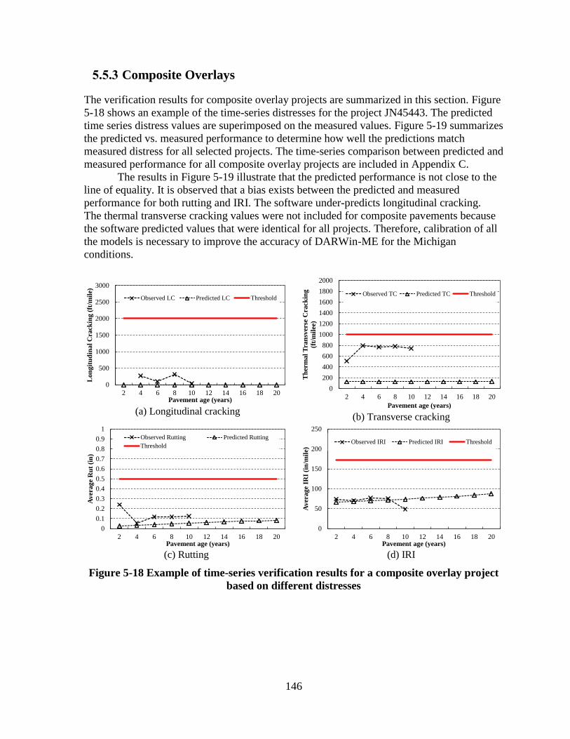
146
5.5.3 Composite Overlays
The verification results for composite overlay projects are summarized in this section. Figure
5-18 shows an example of the time-series distresses for the project JN45443. The predicted
time series distress values are superimposed on the measured values. Figure 5-19 summarizes
the predicted vs. measured performance to determine how well the predictions match
measured distress for all selected projects. The time-series comparison between predicted and
measured performance for all composite overlay projects are included in Appendix C.
The results in Figure 5-19 illustrate that the predicted performance is not close to the
line of equality. It is observed that a bias exists between the predicted and measured
performance for both rutting and IRI. The software under-predicts longitudinal cracking.
The thermal transverse cracking values were not included for composite pavements because
the software predicted values that were identical for all projects. Therefore, calibration of all
the models is necessary to improve the accuracy of DARWin-ME for the Michigan
conditions.
(a) Longitudinal cracking (b) Transverse cracking
(c) Rutting
(d) IRI
Figure 5-18 Example of time-series verification results for a composite overlay project
based on different distresses
0
500
1000
1500
2000
2500
3000
2 4 6 8 10 12 14 16 18 20
Lo
ng
itu
din
al
Cra
ckin
g (
ft/m
ile)
Pavement age (years)
Observed LC Predicted LC Threshold
0
200
400
600
800
1000
1200
1400
1600
1800
2000
2 4 6 8 10 12 14 16 18 20
Th
erm
al
Tra
nsv
erse
Cra
ckin
g
(ft/
mil
ee)
Pavement age (years)
Observed TC Predicted TC Threshold
0
0.1
0.2
0.3
0.4
0.5
0.6
0.7
0.8
0.9
1
2 4 6 8 10 12 14 16 18 20
Av
era
ge
Ru
t (i
n)
Pavement age (years)
Observed Rutting Predicted Rutting
Threshold
0
50
100
150
200
250
2 4 6 8 10 12 14 16 18 20
Aver
age
IRI
(in
/mil
e)
Pavement age (years)
Observed IRI Predicted IRI Threshold
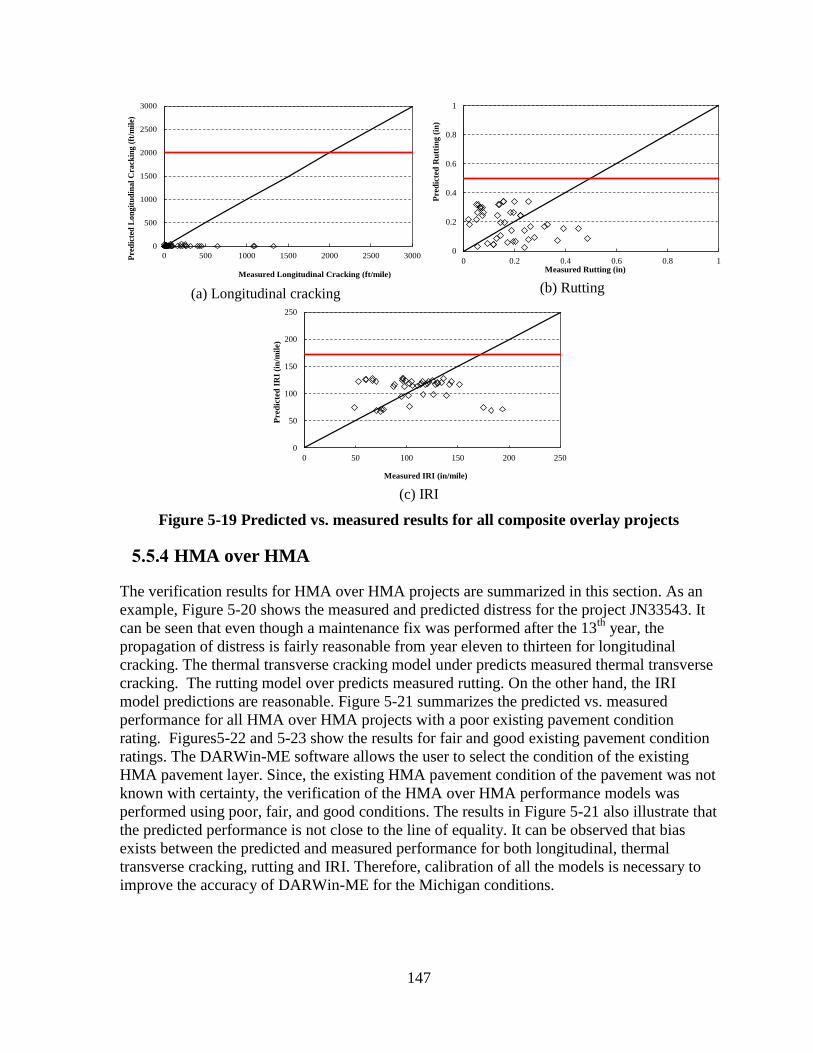
147
(a) Longitudinal cracking
(b) Rutting
(c) IRI
Figure 5-19 Predicted vs. measured results for all composite overlay projects
5.5.4 HMA over HMA
The verification results for HMA over HMA projects are summarized in this section. As an
example, Figure 5-20 shows the measured and predicted distress for the project JN33543. It
can be seen that even though a maintenance fix was performed after the 13th
year, the
propagation of distress is fairly reasonable from year eleven to thirteen for longitudinal
cracking. The thermal transverse cracking model under predicts measured thermal transverse
cracking. The rutting model over predicts measured rutting. On the other hand, the IRI
model predictions are reasonable. Figure 5-21 summarizes the predicted vs. measured
performance for all HMA over HMA projects with a poor existing pavement condition
rating. Figures5-22 and 5-23 show the results for fair and good existing pavement condition
ratings. The DARWin-ME software allows the user to select the condition of the existing
HMA pavement layer. Since, the existing HMA pavement condition of the pavement was not
known with certainty, the verification of the HMA over HMA performance models was
performed using poor, fair, and good conditions. The results in Figure 5-21 also illustrate that
the predicted performance is not close to the line of equality. It can be observed that bias
exists between the predicted and measured performance for both longitudinal, thermal
transverse cracking, rutting and IRI. Therefore, calibration of all the models is necessary to
improve the accuracy of DARWin-ME for the Michigan conditions.
0
500
1000
1500
2000
2500
3000
0 500 1000 1500 2000 2500 3000Pre
dic
ted
Lo
ng
itu
din
al
Cra
ckin
g (
ft/m
ile)
Measured Longitudinal Cracking (ft/mile)
0
0.2
0.4
0.6
0.8
1
0 0.2 0.4 0.6 0.8 1
Pre
dic
ted
Ru
ttin
g (
in)
Measured Rutting (in)
0
50
100
150
200
250
0 50 100 150 200 250
Pre
dic
ted
IR
I (i
n/m
ile)
Measured IRI (in/mile)

148
(a) Longitudinal cracking
(b) Transverse cracking
(c) Rutting
(d) IRI
Figure 5-20 Example of time-series verification results for a HMA over HMA project
(a) Longitudinal cracking
(b) Transverse cracking
(c) Rutting
(d) IRI
Figure 5-21 Predicted vs. Measured performance for HMA over HMA with poor
existing condition.
0
500
1000
1500
2000
2500
1 3 5 7 9 11 13 15 17 19
Lon
git
ud
inal
Cra
ckin
g (
ft/m
ile)
Pavement age (years)
Observed LC Predicted LC - PoorThreshold Predicted LC - FairPredicted LC - Good
0
500
1000
1500
2000
2500
1 3 5 7 9 11 13 15 17 19
Th
erm
al
Tra
nsv
erse
Cra
ckin
g
(ft/
mil
e)
Pavement age (years)
Observed TC
Predicted TC - Poor
Threshold
Predicted TC - Fair
Predicted TC - Good
0
0.1
0.2
0.3
0.4
0.5
0.6
0.7
0.8
0.9
1
1 3 5 7 9 11 13 15 17 19
Aver
age
Ru
t (i
n)
Pavement age (years)
Observed Rutting Predicted Rutting - Poor
Threshold Predicted Rutting - Fair
Predicted Rutting - Good
0
50
100
150
200
250
1 3 5 7 9 11 13 15 17 19
Av
era
ge
IRI
(in
/mil
e)
Pavement age (years)
Observed IRI Predicted IRI - PoorThreshold Predicted IRI - FairPredicted IRI - Good
0
1000
2000
3000
4000
5000
0 1000 2000 3000 4000 5000
Pre
dic
ted
Lo
ng
itu
din
al
Cra
ckin
g
(ft/
mil
e)
Measured Longitudinal Cracking (ft/mile)
0
1000
2000
3000
4000
5000
0 1000 2000 3000 4000 5000
Pre
dic
ted
Tra
nsv
erse
Cra
ckin
g
(ft/
mil
e)
Measured Transverse Cracking (ft/mile)
0.0
0.2
0.4
0.6
0.8
1.0
0 0.2 0.4 0.6 0.8 1
Pre
dic
ted
Ru
ttin
g (
in)
Measured Rutting (in)
0
50
100
150
200
250
0 50 100 150 200 250
Pre
dic
ted
IR
I (i
n/m
ile)
Measured IRI (in/mile)
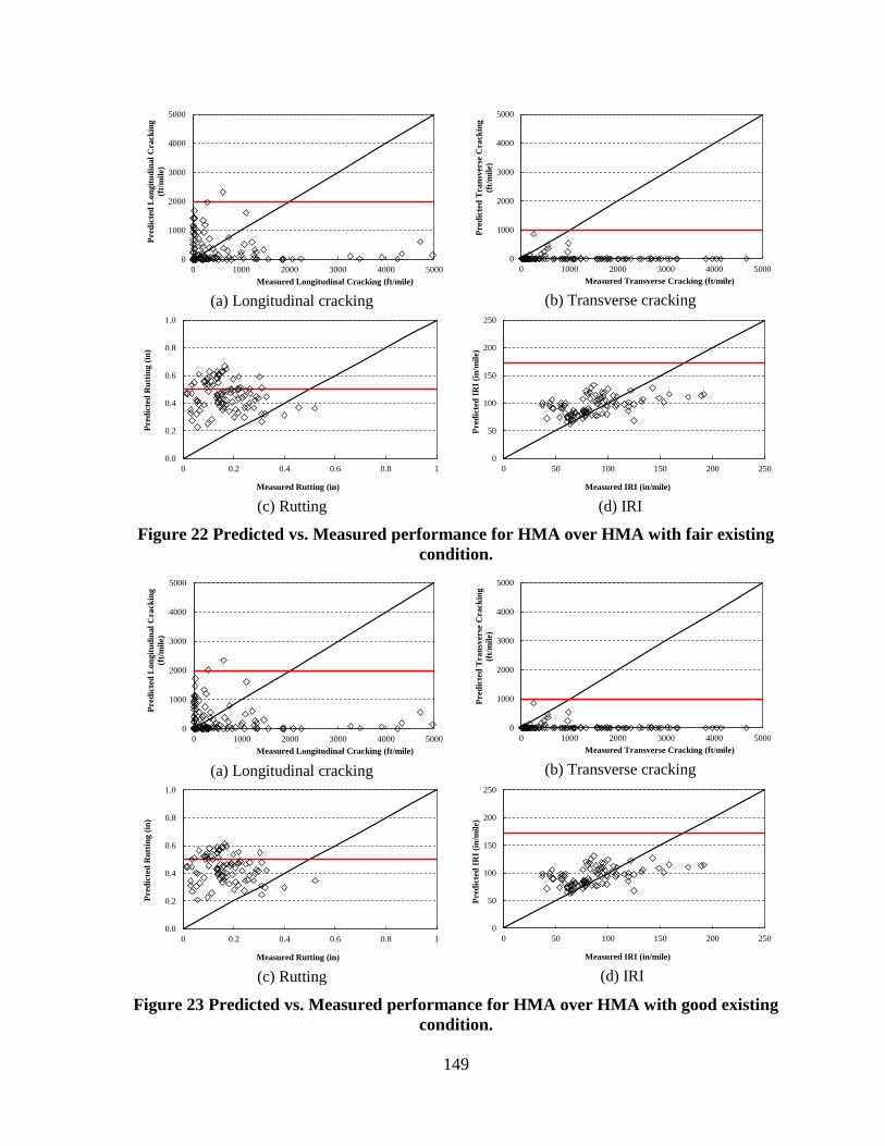
149
(a) Longitudinal cracking
(b) Transverse cracking
(c) Rutting
(d) IRI
Figure 22 Predicted vs. Measured performance for HMA over HMA with fair existing
condition.
(a) Longitudinal cracking
(b) Transverse cracking
(c) Rutting
(d) IRI
Figure 23 Predicted vs. Measured performance for HMA over HMA with good existing
condition.
0
1000
2000
3000
4000
5000
0 1000 2000 3000 4000 5000
Pre
dic
ted
Lo
ng
itu
din
al
Cra
ckin
g
(ft/
mil
e)
Measured Longitudinal Cracking (ft/mile)
0
1000
2000
3000
4000
5000
0 1000 2000 3000 4000 5000
Pre
dic
ted
Tra
nsv
erse
Cra
ckin
g
(ft/
mil
e)
Measured Transverse Cracking (ft/mile)
0.0
0.2
0.4
0.6
0.8
1.0
0 0.2 0.4 0.6 0.8 1
Pre
dic
ted
Ru
ttin
g (
in)
Measured Rutting (in)
0
50
100
150
200
250
0 50 100 150 200 250P
red
icte
d I
RI
(in
/mil
e)
Measured IRI (in/mile)
0
1000
2000
3000
4000
5000
0 1000 2000 3000 4000 5000
Pre
dic
ted
Lo
ng
itu
din
al
Cra
ckin
g
(ft/
mil
e)
Measured Longitudinal Cracking (ft/mile)
0
1000
2000
3000
4000
5000
0 1000 2000 3000 4000 5000
Pred
icte
d T
ran
sverse
Cra
ck
ing
(ft/
mil
e)
Measured Transverse Cracking (ft/mile)
0.0
0.2
0.4
0.6
0.8
1.0
0 0.2 0.4 0.6 0.8 1
Pred
icte
d R
utt
ing
(in
)
Measured Rutting (in)
0
50
100
150
200
250
0 50 100 150 200 250
Pre
dic
ted
IR
I (i
n/m
ile)
Measured IRI (in/mile)

150
5.6 SUMMARY
Verification of the M-E PDG/DARWin-ME performance models are necessary to determine
how well the models predict measured pavement performance for Michigan conditions. In
this chapter, the following sequential steps for the verification process were presented:
1. Identify projects in different regions in the State based on local pavement design and
construction practices.
2. Extract the measured pavement performance data for each project from the MDOT
Pavement Management System (PMS) and Sensor database.
3. Obtain all input data related to pavement materials, cross-section, traffic and climatic
conditions for the identified projects.
4. Compare the measured and predicted performances for each project to identify the
local calibration needs.
The verification of the performance prediction models based on the selected projects
for different rehabilitation options show the need for local calibration. This calibration will
be executed in Task 3 of the project. It should be noted that work accomplished in this task
will facilitate the calibration process due to the following reasons:
All of the identified projects can be used in the local calibration.
The custom PMS and sensor databases developed in this task can be used to further
identify additional road segments based on distress magnitudes instead of
construction records for local calibration (if needed).

151
CHAPTER 6 - CONCLUSIONS AND RECOMMENDATIONS
6.1 SUMMARY
The main objectives of Part 2 of the project were to determine the impact of various input
variables on the predicted pavement performance for the selected rehabilitation design
alternatives in the MEPDG/DARWin-ME, and to verify the pavement performance models
for MDOT rehabilitation design practice. Therefore, the significant inputs related to material
characterization, existing pavement condition, and structural design for the selected
rehabilitation options were identified. Subsequently, the accuracy of the rehabilitation
performance models was evaluated by comparing measured and predicted performance.
The overarching findings from the sensitivity analyses performed in Part 2 for
different rehabilitation options in the MEPDG/DARWin-ME of the study are:
HMA over HMA: the overlay thickness and HMA volumetrics are the most significant
inputs for the overlay layer while the existing HMA thickness and pavement
condition rating have a significant effect on the predicted pavement performance
among the inputs related to the existing pavement structure.
Composite pavements: the overlay thickness and HMA air voids are significant inputs
for the overlay layer. In addition, among the inputs related to the existing intact PCC
pavement, the existing PCC thickness has a significant effect on the predicted
pavement performance.
Rubblized pavements: the HMA thickness, air voids and effective binder content are
the most significant inputs for the overlay layer. While none of the inputs related to
the existing PCC layer have shown a significant impact on the predicted performance,
the results show that the existing PCC layer modulus is important for alligator
cracking and IRI.
Unbonded overlays: all overlay (i.e. the new layer) related inputs significantly impact
the predicted cracking performance while the modulus of subgrade reaction (k-value)
is the most important among inputs related to existing layers.
The interaction between overlay air voids and existing pavement thickness
significantly impacts all performance measures among HMA rehabilitation options. The
interaction between overlay thickness and existing PCC layer modulus has the most
significant effect on unbonded overlay predicted performance. It should be noted that all
analyses were conducted using input ranges reflecting Michigan practices.
The verification of the performance prediction models based on the selected projects
for different rehabilitation options show the need for local calibration. All of the identified
projects used for verification will be utilized in Task 3 for local calibration. Based on the
results of the analyses, various conclusions and recommendations were made and are
presented in the next sections.
152
6.2 CONCLUSIONS
Based on the results of the analyses performed in Part 2 tasks, various conclusions were
drawn. These conclusions can be divided into the following three broad topics:
Issues related to the MEPDG/DARWin-ME software
Identification of significant inputs based on sensitivity analyses
Verification of the MEPDG/DARWin-ME rehabilitation performance models
6.2.1 The MEPDG/DARWin-ME Software Issues
Several issues were encountered while running the MEPDG/DARWin-ME software. These
concerns were related to certain structural and material properties. In addition,
reasonableness of certain inputs was investigated whenever unusual results were encountered
during the analyses. These concerns include:
1. The software internally limits the existing PCC elastic modulus because higher values
produce counter intuitive results. Therefore, the recommended value of 3,000,000 psi
should be considered as the upper bound limit for elastic modulus.
2. The software reduces the subgrade resilient modulus (MR) value by a fixed factor
depending on the soil type; fine or coarse. If the design MR is used as a direct input in
the MEPDG/DARWin-ME, the MR values will be reduced internally to reflect
laboratory determined MR (for levels 2 and 3). It should be noted that in the
DARWin-ME the reduction factor can be specified by the user for level 1 while the
software uses an internal reduction factor for unbound layers when using levels 2 &
3.
3. In the MEPDG/DARWin-ME the HMA interlayer modulus and thickness have
insignificant impact on the equivalent thickness, especially within the practical range
of 1 to 3 inches for interlayer thickness. This implies that the interlayer thickness and
stiffness have no significant impact on the predicted performance.
6.2.2 Sensitivity Analyses
The main objective in this task was to evaluate the impact of the inputs specific to various
rehabilitation options on the predicted performance. To accomplish this goal, the following
types of sensitivity analyses were performed:
1. Preliminary sensitivity
2. Detailed sensitivity
3. Global sensitivity
4. Satellite studies
Each sensitivity analysis has a unique contribution to the overall understanding in
determining the impact of design inputs on the predicted pavement performance. The
outcome of the preliminary sensitivity resulted in the identification of significant inputs
related to the existing pavement layers. Subsequently, these inputs were combined with the

153
significant inputs for the new pavement layer (overlay) to conduct the detailed sensitivity.
The outcome from the detailed sensitivity analyses include the significant main and
interactive effects (ANOVA) between the inputs related to the existing and overlay layers. It
should be noted that the statistical and practical significant interactive effects were only
investigated for the inputs related to the existing layer, overlay layer and a combination of
existing and overlay layers.
Finally, the global sensitivity analysis was performed based on the results from the
detailed sensitivity analysis. The global sensitivity analysis (GSA) is more robust because of
the following reasons:
a. Main and interaction results are based on the entire domain of each input variable.
b. The importance of each input can be quantified using normalized sensitivity index
(NSI).
c. Relative importance of each design input can be determined.
In this report, the term “sensitive” implies changes in the output (predicted
performance) with respect to change in the input values. On the other hand, the term
“significant” implies changes in the design input values that result in substantial changes in
the predicted performance.
6.2.2.1 Preliminary sensitivity
Table 6-1summarizes the significant inputs from preliminary sensitivity analyses for the
selected rehabilitation options. These inputs only characterize the existing pavement. The
results show that existing surface layer thickness and existing pavement structural capacity
are the most important inputs for all rehabilitation options.
Table 6-1 List of significant inputs from preliminary sensitivity analysis
Rehabilitation option Significant inputs
HMA over HMA Existing HMA condition rating
Existing HMA thickness
HMA over JPCP
(Composite)
Existing PCC thickness
Existing PCC flexural strength
JPCP over JPCP
(Unbonded overlay) Existing PCC thickness
CRCP over HMA Existing HMA thickness
CRCP over JPCP
Existing PCC thickness
Existing PCC strength
Subgrade k-value
6.2.2.2 Detailed sensitivity
The detailed sensitivity analyses included the significant variables identified in preliminary
analyses in addition to the significant inputs previously identified for new pavement layers.

154
Full factorials were designed to determine statistically significant main and two-way
interaction effects. The results of the sensitivity analyses show that the existing pavement
condition rating and existing thickness for HMA over HMA is critical for all performance
measures. On the other hand, existing PCC modulus and thickness are important in
determining the performance of HMA overlay over intact and rubblized PCC. For a given
condition of the existing pavement, HMA overlay volumetric properties, binder type and
amount, and thickness play a significant role. In addition, HMA volumetrics, binder type and
amount, and thickness should be carefully selected for the overlays to mitigate various
distresses whether the existing pavement is intact or rubblized concrete.
For unbonded overlays, the results of the sensitivity analyses show that the existing
pavement condition (in terms of E) is critical for predicting cracking performance. Higher
MOR (within reason) and thickness of overlay will limit the cracking. However, if the
existing foundation is weak, a better strategy to reduce the unbonded overlay cracking would
be to either increase PCC MOR or thickness, and use concrete with lower CTE. Table 6-2
presents the summary of significant input variable based on the detailed sensitivity analysis.
Table 6-2 List of significant inputs from detailed sensitivity analysis
Rehabilitation option Significant inputs
HMA over HMA
Existing HMA condition rating
Existing HMA thickness
Granular base and subgrade modulus
Overlay air voids
Overlay effective binder
Overlay binder PG
Overlay thickness
HMA over JPCP
(Composite)
Existing PCC thickness
Existing PCC flexural strength
Climate
Overlay air voids
Overlay binder PG
Overlay thickness
HMA over JPCP fractured
(Rubblized)
Existing PCC thickness
Existing PCC elastic modulus
Overlay air voids
Overlay effective binder
Overlay binder PG
Overlay thickness
JPCP over JPCP
(Unbonded overlay)
Existing PCC thickness
Existing PCC elastic modulus
Existing modulus of subgrade reaction
Overlay MOR
Overlay thickness
Overlay CTE
Overlay joint spacing
155
6.2.2.3 Global sensitivity analysis
Four rehabilitation options were considered in global sensitivity analysis (GSA) similar to the
preliminary and the detailed sensitivity analyses. First, the relative contributions of the design
inputs for various performance measures were identified and discussed. Second, the main
effect of design inputs for a base case was investigated. Finally the interactive effect of the
design inputs was studied for all performance measures within each rehabilitation option.
The results are summarized based on the main effects determined through the
maximum NSI values. The input variables are ranked based on their relative impact on
different performance measures. The following are the findings based on the main effects of
input variables:
HMA over HMA
In general, the overlay thickness and HMA volumetrics (air voids and effective
binder contents) are the most significant inputs affecting the predicted performance
for the overlay layer
The existing pavement thickness and condition rating have significant effect among
the existing pavement related inputs. Table 6-3 shows the list of significant inputs
along with the ranking and NSI values.
Table 6-3 List of significant inputs — HMA over HMA
Input variables Ranking (NSI)
Overlay air voids 1 (6)
Existing thickness 2 (5)
Overlay thickness 3 (4)
Existing pavement condition rating 4 (4)
Overlay effective binder 5 (2)
Subgrade modulus 6 (2)
Subbase modulus 7 (1)
Composite pavement
The overlay thickness and HMA air voids are the most significant inputs for the
overlay layer
The existing pavement thickness and existing PCC layer modulus have significant
effect on predicted performance among the existing pavement related inputs. Table 6-
4 shows the list of significant inputs along with the ranking and NSI values.
Table 6-4 List of significant inputs — Composite pavement
Inputs Ranking (NSI)
Overlay air voids 1 (9)
Overlay thickness 2 (2)
Existing PCC thickness 3 (1)
Rubblized pavement
The HMA air voids and effective binder content are the most significant inputs for the
overlay layer
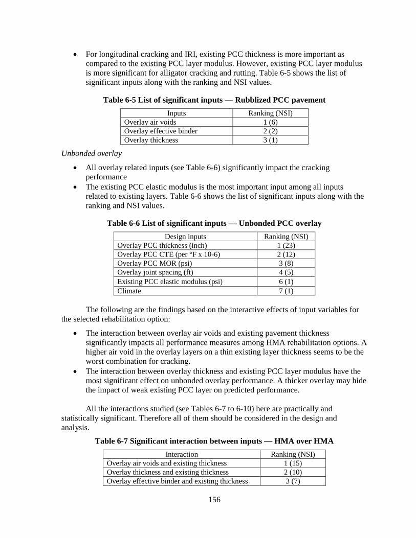
156
For longitudinal cracking and IRI, existing PCC thickness is more important as
compared to the existing PCC layer modulus. However, existing PCC layer modulus
is more significant for alligator cracking and rutting. Table 6-5 shows the list of
significant inputs along with the ranking and NSI values.
Table 6-5 List of significant inputs — Rubblized PCC pavement
Inputs Ranking (NSI)
Overlay air voids 1 (6)
Overlay effective binder 2 (2)
Overlay thickness 3 (1)
Unbonded overlay
All overlay related inputs (see Table 6-6) significantly impact the cracking
performance
The existing PCC elastic modulus is the most important input among all inputs
related to existing layers. Table 6-6 shows the list of significant inputs along with the
ranking and NSI values.
Table 6-6 List of significant inputs — Unbonded PCC overlay
Design inputs Ranking (NSI)
Overlay PCC thickness (inch) 1 (23)
Overlay PCC CTE (per °F x 10-6) 2 (12)
Overlay PCC MOR (psi) 3 (8)
Overlay joint spacing (ft) 4 (5)
Existing PCC elastic modulus (psi) 6 (1)
Climate 7 (1)
The following are the findings based on the interactive effects of input variables for
the selected rehabilitation option:
The interaction between overlay air voids and existing pavement thickness
significantly impacts all performance measures among HMA rehabilitation options. A
higher air void in the overlay layers on a thin existing layer thickness seems to be the
worst combination for cracking.
The interaction between overlay thickness and existing PCC layer modulus have the
most significant effect on unbonded overlay performance. A thicker overlay may hide
the impact of weak existing PCC layer on predicted performance.
All the interactions studied (see Tables 6-7 to 6-10) here are practically and
statistically significant. Therefore all of them should be considered in the design and
analysis.
Table 6-7 Significant interaction between inputs — HMA over HMA
Interaction Ranking (NSI)
Overlay air voids and existing thickness 1 (15)
Overlay thickness and existing thickness 2 (10)
Overlay effective binder and existing thickness 3 (7)
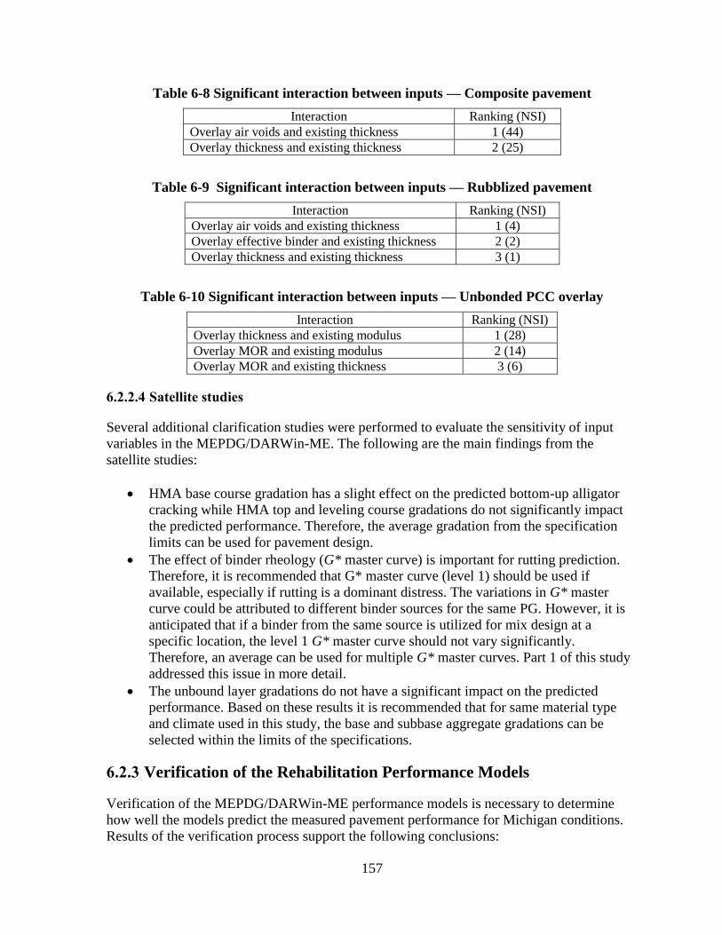
157
Table 6-8 Significant interaction between inputs — Composite pavement
Interaction Ranking (NSI)
Overlay air voids and existing thickness 1 (44)
Overlay thickness and existing thickness 2 (25)
Table 6-9 Significant interaction between inputs — Rubblized pavement
Interaction Ranking (NSI)
Overlay air voids and existing thickness 1 (4)
Overlay effective binder and existing thickness 2 (2)
Overlay thickness and existing thickness 3 (1)
Table 6-10 Significant interaction between inputs — Unbonded PCC overlay
Interaction Ranking (NSI)
Overlay thickness and existing modulus 1 (28)
Overlay MOR and existing modulus 2 (14)
Overlay MOR and existing thickness 3 (6)
6.2.2.4 Satellite studies
Several additional clarification studies were performed to evaluate the sensitivity of input
variables in the MEPDG/DARWin-ME. The following are the main findings from the
satellite studies:
HMA base course gradation has a slight effect on the predicted bottom-up alligator
cracking while HMA top and leveling course gradations do not significantly impact
the predicted performance. Therefore, the average gradation from the specification
limits can be used for pavement design.
The effect of binder rheology (G* master curve) is important for rutting prediction.
Therefore, it is recommended that G* master curve (level 1) should be used if
available, especially if rutting is a dominant distress. The variations in G* master
curve could be attributed to different binder sources for the same PG. However, it is
anticipated that if a binder from the same source is utilized for mix design at a
specific location, the level 1 G* master curve should not vary significantly.
Therefore, an average can be used for multiple G* master curves. Part 1 of this study
addressed this issue in more detail.
The unbound layer gradations do not have a significant impact on the predicted
performance. Based on these results it is recommended that for same material type
and climate used in this study, the base and subbase aggregate gradations can be
selected within the limits of the specifications.
6.2.3 Verification of the Rehabilitation Performance Models
Verification of the MEPDG/DARWin-ME performance models is necessary to determine
how well the models predict the measured pavement performance for Michigan conditions.
Results of the verification process support the following conclusions:
158
For the unbonded overlay, the MEPDG/DARWin-ME software under-predicts the
measured cracking and faulting. The IRI predicted values were closer to the measured
performance; however, bias still exists.
For rubblized pavements, the software under-predicts longitudinal and transverse
cracking for most of the pavement sections while it over-predicts the measured
distresses for rutting and IRI.
For composite pavements, the one-to-one plot between the predicted and measured
performance for rutting and IRI showed higher variability (i.e., more error). Also, the
software under-predicted the longitudinal cracking.
For HMA over HMA bias exists between the predicted and measured performance for
rutting and IRI i.e., the software over predicts the measured performance. While
longitudinal cracking showed larger error, thermal transverse cracking was under-
predicted.
The validation of the performance prediction models based on the selected projects
for different rehabilitation options show the need for local calibration. This calibration will
be executed in Part 3 of the research study. It should be noted that work accomplished in this
task will facilitate the calibration process due to the following reasons:
All of the identified projects can be used in the local calibration.
The custom PMS and sensor databases developed in this task can be used to further
identify additional road segments based on distress magnitudes instead of
construction records for local calibration (if needed).
6.3 RECOMMENDATIONS
The following are the recommendations based on the findings from Part 2:
1. For unbonded overlays, the existing PCC elastic modulus input should not exceed a
value of 3,000,000 psi.
2. An average HMA gradation from the specification limits should be used for pavement
design.
3. The average G* master curve (level 1) should be used if available for a binder from a
source, especially if rutting is the dominant distress.
4. For unbound layers, base and subbase aggregate gradations should be selected within
the limits of the specifications.
5. It is recommended that the following rehabilitation option in the DARWin-ME
should be used for design until local calibration is performed.
a. HMA over HMA
b. Composite overlays
c. Rubblized overlays
d. Unbonded PCC overlays
6. The use of falling weight deflectometer (FWD) is recommended to characterize the
existing pavement, especially for flexible pavements with high traffic volume. The
FWD testing guidelines for sensor configuration, number of drops, testing frequency
and temperature measurements are outlined in Chapter 3. The guidelines are

159
recommended in the short-term while modifications should be made in the long-term
based on the local experience.
7. The use of ground penetration radar (GPR) for estimating the existing pavement layer
thicknesses in conjunction with FWD is recommended to enhance the back-
calculation accuracy and testing efficiency.
8. The load pulse of the MDOT FWD equipment should be used to calculate the
frequency based on the equation: 1
2f
t .
9. Further investigation is needed during the local calibration of the performance models
(Part 3 of the study) to evaluate the appropriateness of both backcalculated and design
subgrade MR values.
6.4 IMPLEMENTATION
Based on the conclusions and recommendations of Part II study, the following are
recommendations for the implementation of the DARWin-ME in the state of Michigan:
Increase the use of FWD for backcalculation of layer moduli to characterize existing
pavement conditions for all the rehabilitation options adopted in Michigan is
warranted, especially for high traffic volume roads (interstates and freeways).
PMS distress data and unit conversion is also necessary to ensure compatibility
between MDOT measured and DARWin-ME predicted distresses in the long-term for
implementation of the new design methodology (see Tables 6-11 and 6-12). The units
can be converted by using the equations mentioned in Chapter 5. The results of
conversion should be stored separately in the database for the selected PD’s listed
Chapter 5. Sensor data (IRI, rut depth and faulting) do not need any further
conversion because of their compatibility with DARWin-ME.
Table 6-11 Flexible pavement distresses
Flexible pavement
distresses
MDOT
units
DARWin-ME
units
Conversion
needed?
IRI in/mile in/mile No
Top-down cracking miles ft/mile Yes
Bottom-up cracking miles % area Yes
Thermal cracking No. of
occurrences ft/mile Yes
Rutting in in No
Reflective cracking None % area No
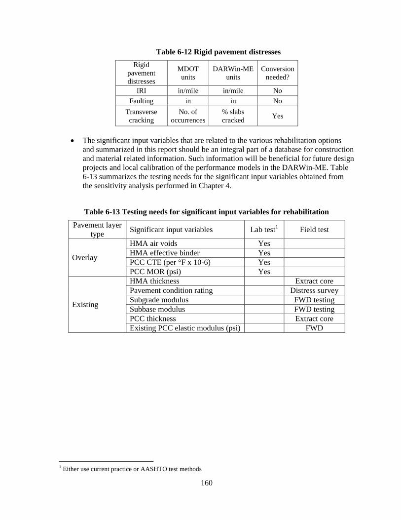
160
Table 6-12 Rigid pavement distresses
Rigid
pavement
distresses
MDOT
units
DARWin-ME
units
Conversion
needed?
IRI in/mile in/mile No
Faulting in in No
Transverse
cracking
No. of
occurrences
% slabs
cracked Yes
The significant input variables that are related to the various rehabilitation options
and summarized in this report should be an integral part of a database for construction
and material related information. Such information will be beneficial for future design
projects and local calibration of the performance models in the DARWin-ME. Table
6-13 summarizes the testing needs for the significant input variables obtained from
the sensitivity analysis performed in Chapter 4.
Table 6-13 Testing needs for significant input variables for rehabilitation
Pavement layer
type Significant input variables Lab test
1 Field test
Overlay
HMA air voids Yes
HMA effective binder Yes
PCC CTE (per °F x 10-6) Yes
PCC MOR (psi) Yes
Existing
HMA thickness Extract core
Pavement condition rating Distress survey
Subgrade modulus FWD testing
Subbase modulus FWD testing
PCC thickness Extract core
Existing PCC elastic modulus (psi) FWD
1 Either use current practice or AASHTO test methods

161
REFERENCES
CHAPTER 2
1. Haider, S. W., H. K. Salama, N. Buch, and K. Chatti, "Significant M-E PDG Design
Inputs for Jointed Plain Concrete Pavements in Michigan," presented at the Fifth
International Conference on Maintenance and Rehabilitation of Pavements and
Technological Control, Park City, Utah, USA, 2007, pp. 79-84.
2. Haider, S. W., H. K. Salama, N. Buch, and K. Chatti, "Influence of Traffic Inputs on
Rigid Pavement Performance Using M-E PDG in the State of Michigan," presented at
the Fifth International Conference on Maintenance and Rehabilitation of Pavements
and Technological Control, Park City, Utah, USA, 2007, pp. 85-90.
3. Buch, N., K. Chatti, S. W. Haider, and A. Manik, "Evaluation of the 1-37A Design
Process for New and Rehabilitated JPCP and HMA Pavements, Final Report,"
Michigan Department of Transportation, Construction and Technology Division, P.O.
Box 30049, Lansing, MI 48909, Lansing, Research Report RC-1516, 2008.
4. Haider, S. W., N. Buch, and K. Chatti, "Evaluation of M-E PDG for Rigid
Pavements—Incorporating the State-of-the-Practice in Michigan," presented at the
9th International Conference on Concrete Pavements San Francisco, California, USA,
2008, pp.
5. Buch, N., S. W. Haider, J. Brown, and K. Chatti, "Characterization of Truck Traffic
in Michigan for the New Mechanistic Empirical Pavemnet Design Guide, Final
Report," Michigan Department of Transportation, Construction and Technology
Division, P.O. Box 30049, Lansing, MI 48909, Lansing, Research Report RC-1537,
2009.
6. Haider, S. W., N. Buch, K. Chatti, and J. Brown, "Development of Traffic Inputs for
Mechanistic-Empirical Pavement Design Guide in Michigan," Transportation
Research Record, vol. 2256, pp. 179-190, 2011.
7. Baladi, G. Y., T. Dawson, and C. Sessions, "Pavement Subgrade MR Design Values
for Michigan’s Seasonal Changes, Final Report," Michigan Department of
Transportation, Construction and Technology Division, P.O. Box 30049, Lansing, MI
48909, Lansing, Research Report RC-1531, 2009.
8. Baladi, G. Y., K. A. Thottempudi, and T. Dawson, "Backcalculation of Unbound
Granular Layer Moduli, Final Report," Michigan Department of Transportation,
Construction and Technology Division, P.O. Box 30049, Lansing, MI 48909,
Lansing, 2010.
9. Schwartz, C. W., R. Li, S. Kim, H. Ceylan, and R. Gopalakrishnan, "Sensitivity
Evaluation of MEPDG Performance Prediction," NCHRP 1-47 Final Report, 2011.
10. Zhou, C., B. Huang, X. Shu, and Q. Dong, "Validating MEPDG with Tennessee
Pavement Performance Data," Journal of Transportation Engineering, vol. 139, pp.
306-312, 2013.
11. NCHRP Project 1-37A, "Guide for Mechanistic-Empirical Design of New and
Rehabilitated Pavement structures," National Cooperative Research Program
(NCHRP), Washington D.C. Final Report, 2004.
162
12. NCHRP Project 1-40B, "Local Calibration Guidance for the Recommended Guide for
Mechanistic-Empirical Pavement Design of New and Rehabilitated Pavement
Structures," Final NCHRP Report 2009.
13. AASHTO, "Mechanistic-Empirical Pavement Design Guide: A Manual of Practice:
Interim Edition," American Association of State Highway and Transportation
Officials 2008.
CHAPTER 3
1. AASHTO, "Mechanistic-Empirical Pavement Design Guide: A Manual of Practice:
Interim Edition," American Association of State Highway and Transportation
Officials 2008.
2. NCHRP Project 1-37A, "Guide for Mechanistic-Empirical Design of New and
Rehabilitated Pavement structures," National Cooperative Research Program
(NCHRP), Washington D.C. Final Report, 2004.
3. Tompkins, D., P. Saxena, A. Gotlif, and L. Khazanovich, "Modification of
Mechanistic-Empirical Pavement Design Guide Procedure for Two-Lift Composite
Concrete Pavements," 2012.
4. Smith, K. D., J. E. Bruinsma, M. J. Wade, K. Chatti, J. M. Vandenbossche, and H. T.
Yu, "Using Falling Weight Deflectometer Data with Mechanistic-Empirical Design
and Analysis, Volume 1: Final Report," Federal Highway Administration, 1200 New
Jersey Avenue, SE, Washington, DC 20590 2010.
5. Pierce, L. M., K. D. Smith, J. E. Bruinsma, M. J. Wade, K. Chatti, and J. M.
Vandenbossche, "Using Falling Weight Deflectometer Data with Mechanistic-
Empirical Design and Analysis, Volume 3: Guidelines for Deflection Testing,
Analysis, and Interpretation," Federal Highway Administration, 1200 New Jersey
Avenue, SE, Washington, DC 20590 2010.
6. Chatti, K., M. Kutay, and L. Lei, "Relationships between Laboratory‐Measured and
Field‐Derived Properties of Pavement Layers," 2011.
CHAPTER 4
1. Buch, N., K. Chatti, S. W. Haider, and A. Manik, "Evaluation of the 1-37A Design
Process for New and Rehabilitated JPCP and HMA Pavements, Final Report,"
Michigan Department of Transportation, Construction and Technology Division, P.O.
Box 30049, Lansing, MI 48909, Lansing, Research Report RC-1516, 2008.
2. Haider, S. W., N. Buch, and K. Chatti, "Evaluation of M-E PDG for Rigid
Pavements—Incorporating the State-of-the-Practice in Michigan," presented at the
9th International Conference on Concrete Pavements San Francisco, California, USA,
2008, pp.
3. Schwartz, C. W., R. Li, S. Kim, H. Ceylan, and R. Gopalakrishnan, "Sensitivity
Evaluation of MEPDG Performance Prediction," NCHRP 1-47 Final Report, 2011.
4. Kutay, E. and A. Jamrah, "Preparation for Implementation of the Mechanistic-
Empirical Pavement Design Guide in Michiagn: Part 1 - HMA Mixture
Characterization," Michigan Department of Transportation, 425 West Ottawa, P.O.
Box 30050 Lansing, MI 48909, Lansing, Research Report ORBP OR10-022, 2012.
163
5. NCHRP Project 1-37A, "Guide for Mechanistic-Empirical Design of New and
Rehabilitated Pavement structures," National Cooperative Research Program
(NCHRP), Washington D.C. Final Report, 2004.
6. Rauhut, J. B., A. Eltahan, and A. L. Simpson, "Common Characteristics of Good and
Poorly Performing AC Pavements," Federal Highway Administration, FHWA-RD-
99-193, December 1999.
7. Khazanovich, L., D. M, B. R, and M. T, "Common Characteristics of Good and
Poorly Performing PCC Pavements," Federal Highway Administration, FHWA-RD-
97-131, 1998.
8. Haider, S. W., N. Buch, K. Chatti, and J. Brown, "Development of Traffic Inputs for
Mechanistic-Empirical Pavement Design Guide in Michigan," Transportation
Research Record, vol. 2256, pp. 179-190, 2011.
9. Buch, N., S. W. Haider, J. Brown, and K. Chatti, "Characterization of Truck Traffic
in Michigan for the New Mechanistic Empirical Pavemnet Design Guide, Final
Report," Michigan Department of Transportation, Construction and Technology
Division, P.O. Box 30049, Lansing, MI 48909, Lansing, Research Report RC-1537,
2009.
10. AASHTO, "Mechanistic-Empirical Pavement Design Guide: A Manual of Practice:
Interim Edition," American Association of State Highway and Transportation
Officials 2008.
11. Weckman, G., D. Millie, C. Ganduri, M. Rangwala, W. Young, M. Rinder, and G.
Fahnenstiel, "Knowledge extraction from the neural ‘black box’in ecological
monitoring," Journal of Industrial and Systems Engineering, vol. 3, pp. 38-55, 2009.