Ch. 4 – Continuous Random Variables and Probability Distributions

4.1 – Probability Density Functions A continuous random variable is a random variable with an interval of real numbers for its range.

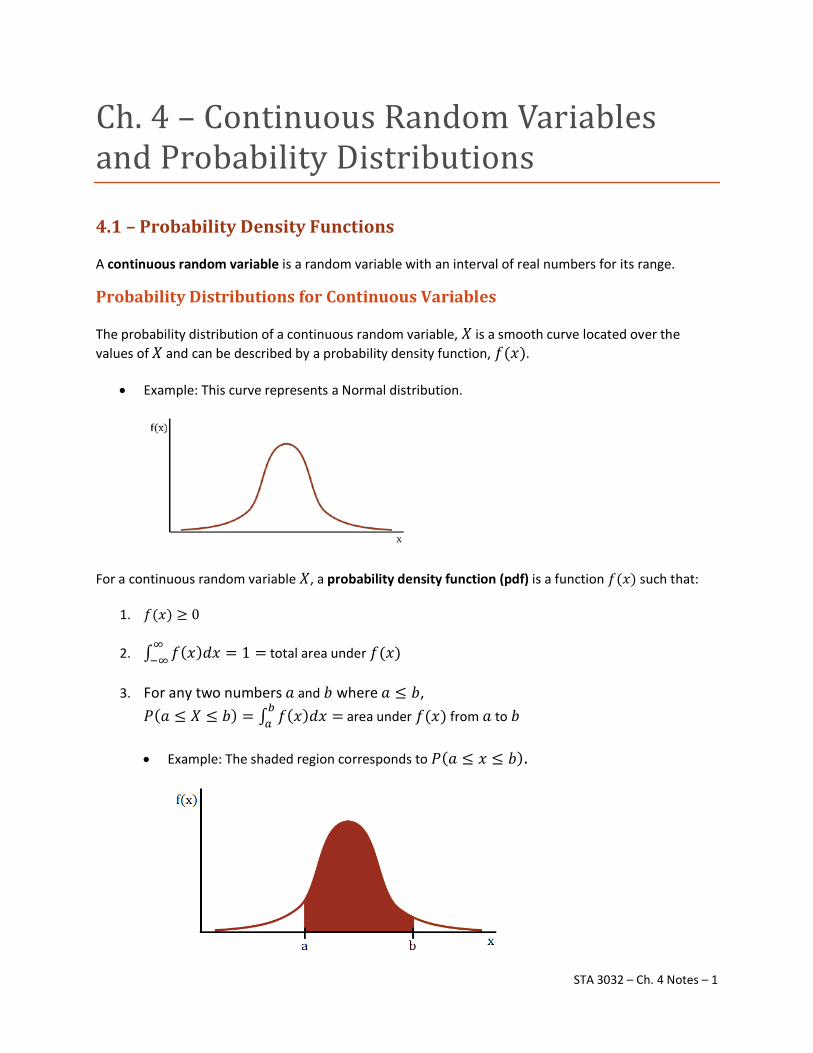
Probability Distributions for Continuous Variables The probability distribution of a continuous random variable, 𝑋 is a smooth curve located over the values of 𝑋 and can be described by a probability density function, 𝑓(𝑥).

• Example: This curve represents a Normal distribution.

For a continuous random variable 𝑋, a probability density function (pdf) is a function 𝑓(𝑥) such that:

1. 𝑓(𝑥) ≥ 0

2. ∫ 𝑓(𝑥)𝑑𝑥 = 1∞−∞ = total area under 𝑓(𝑥)

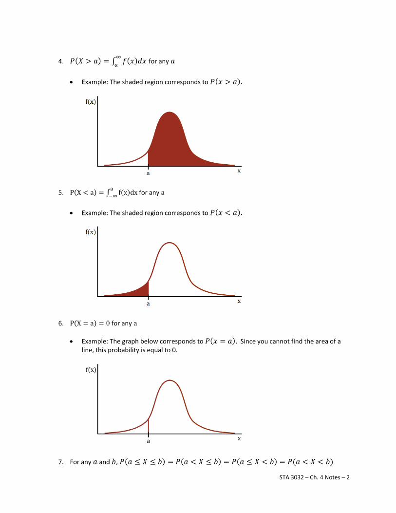
3. For any two numbers 𝑎 and 𝑏 where 𝑎 ≤ 𝑏,

𝑃(𝑎 ≤ 𝑋 ≤ 𝑏) = ∫ 𝑓(𝑥)𝑑𝑥 =𝑏𝑎 area under 𝑓(𝑥) from 𝑎 to 𝑏

• Example: The shaded region corresponds to 𝑃(𝑎 ≤ 𝑥 ≤ 𝑏).

STA 3032 – Ch. 4 Notes – 1

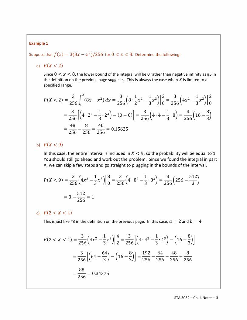
4. 𝑃(𝑋 > 𝑎) = ∫ 𝑓(𝑥)𝑑𝑥∞

𝑎 for any 𝑎

• Example: The shaded region corresponds to 𝑃(𝑥 > 𝑎).

5. P(X < a) = ∫ f(x)dxa−∞ for any a

• Example: The shaded region corresponds to 𝑃(𝑥 < 𝑎).

6. P(X = a) = 0 for any a

• Example: The graph below corresponds to 𝑃(𝑥 = 𝑎). Since you cannot find the area of a line, this probability is equal to 0.

7. For any 𝑎 and 𝑏, 𝑃(𝑎 ≤ 𝑋 ≤ 𝑏) = 𝑃(𝑎 < 𝑋 ≤ 𝑏) = 𝑃(𝑎 ≤ 𝑋 < 𝑏) = 𝑃(𝑎 < 𝑋 < 𝑏)

STA 3032 – Ch. 4 Notes – 2

Example 1 Suppose that 𝑓(𝑥) = 3(8𝑥 − 𝑥2)/256 for 0 < 𝑥 < 8. Determine the following:

a) 𝑃(𝑋 < 2)

Since 0 < 𝑥 < 8, the lower bound of the integral will be 0 rather than negative infinity as #5 in the definition on the previous page suggests. This is always the case when 𝑋 is limited to a specified range.

𝑃(𝑋 < 2) =3

256� (8𝑥 − 𝑥2)2

0𝑑𝑥 =

3256

�8 ∙12𝑥2 −

13𝑥3��

20

=3

256�4𝑥2 −

13𝑥3��

20

=3

256��4 ∙ 22 −

13 ∙ 23� − (0 − 0)� =

3256

�4 ∙ 4 −13∙ 8� =

3256

�16 −83�

=48

256−

8256 =

40256 = 0.15625

b) 𝑃(𝑋 < 9)

In this case, the entire interval is included in 𝑋 < 9, so the probability will be equal to 1. You should still go ahead and work out the problem. Since we found the integral in part A, we can skip a few steps and go straight to plugging in the bounds of the interval.

𝑃(𝑋 < 9) =3

256�4𝑥2 −

13 𝑥

3��80 =

3256

�4 ∙ 82 −13 ∙ 83� =

3256

�256 −512

3�

= 3 −512256 = 1

c) 𝑃(2 < 𝑋 < 4)

This is just like #3 in the definition on the previous page. In this case, 𝑎 = 2 and 𝑏 = 4.

𝑃(2 < 𝑋 < 4) =3

256�4𝑥2 −

13 𝑥

3��42 =

3256

��4 ∙ 42 −13 ∙ 43� − �16 −

83��

=3

256��64 −

643� − �16 −

83�� =

192256

−64

256 −48

256 +8

256

=88

256 = 0.34375

STA 3032 – Ch. 4 Notes – 3

Example 1 Continued

d) 𝑃(𝑋 > 6)

Just like in part A, we use the upper bound of the interval instead of infinity when a range is given for 𝑋.

𝑃(𝑋 > 6) =3

256�4𝑥2 −

13𝑥3��

86

=3

256��256 −

5123� − �4 ∙ 62 −

13∙ 63��

= (3 − 2) −3

256(144 − 72) = 1 −

3256 ∙ 72 = 1 −

216256 =

40256 = 0.15625

Continuous Uniform Distribution The simplest continuous distribution is one where all the values in an interval have equal probability.

Probability Density Function of a Continuous Uniform Random Variable Let 𝑋 be a continuous uniform random variable on the interval [𝑎,𝑏] with pdf

𝑓(𝑥) =1

𝑏 − 𝑎 , 𝑎 ≤ 𝑥 ≤ 𝑏

Mean and Variance of a Continuous Uniform Random Variable

𝜇 = 𝐸(𝑋) =𝑎 + 𝑏

2

𝜎2 = 𝑉(𝑋) =(𝑏 − 𝑎)2

12

Note: These formulas are not given in the book, but you can derive them in Exercise 17 on pg. 151. Example 2

Suppose 𝑋 has a continuous uniform distribution over the interval [1.5, 5.5].

a) Determine the mean, variance, and standard deviation of 𝑋.

𝜇 =1.5 + 5.5

2 =72 = 3.5

STA 3032 – Ch. 4 Notes – 4

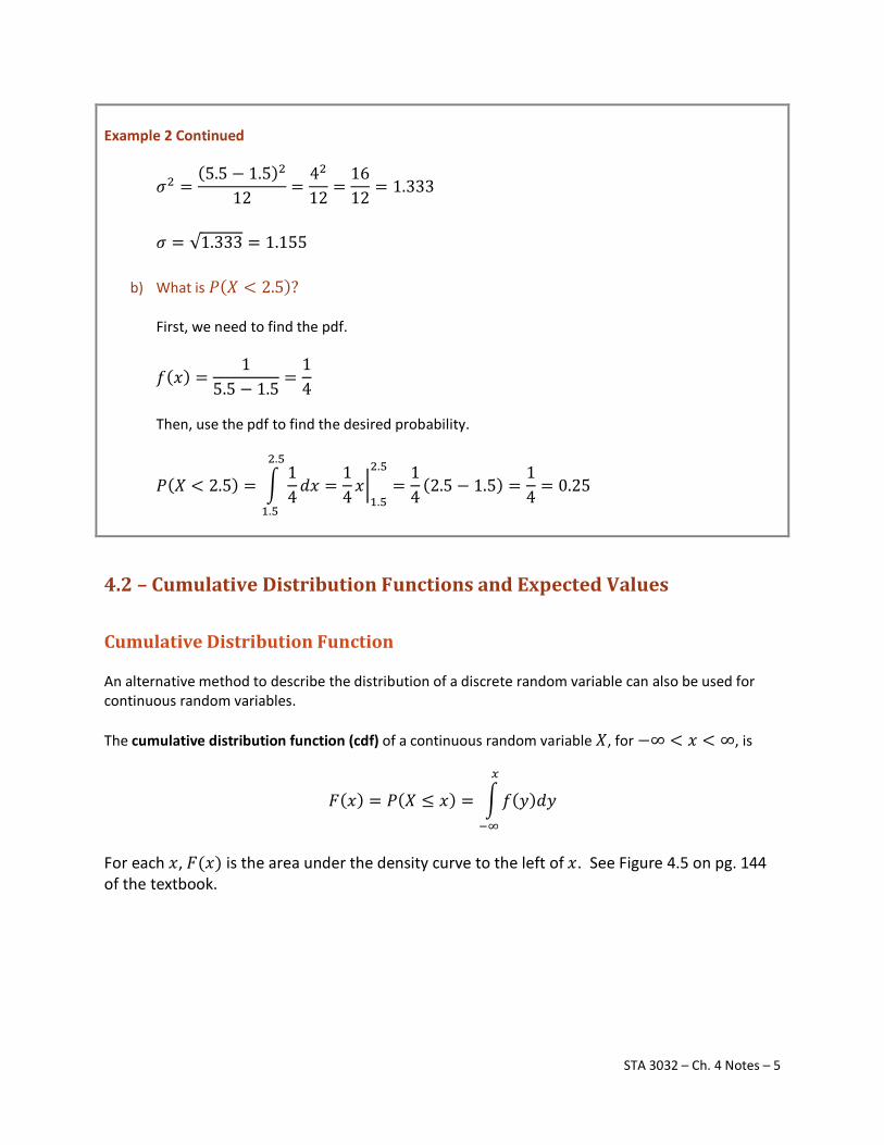
Example 2 Continued

𝜎2 =(5.5 − 1.5)2

12 =42

12 =1612

= 1.333

𝜎 = √1.333 = 1.155

b) What is 𝑃(𝑋 < 2.5)? First, we need to find the pdf.

𝑓(𝑥) =1

5.5 − 1.5=

14

Then, use the pdf to find the desired probability.

𝑃(𝑋 < 2.5) = �14

2.5

1.5

𝑑𝑥 =14 𝑥

�1.5

2.5

=14

(2.5 − 1.5) =14 = 0.25

4.2 – Cumulative Distribution Functions and Expected Values

Cumulative Distribution Function An alternative method to describe the distribution of a discrete random variable can also be used for continuous random variables. The cumulative distribution function (cdf) of a continuous random variable 𝑋, for −∞ < 𝑥 < ∞, is

𝐹(𝑥) = 𝑃(𝑋 ≤ 𝑥) = �𝑓(𝑦)𝑑𝑦𝑥

−∞

For each 𝑥, 𝐹(𝑥) is the area under the density curve to the left of 𝑥. See Figure 4.5 on pg. 144 of the textbook.

STA 3032 – Ch. 4 Notes – 5

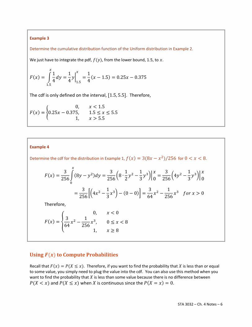
Example 3 Determine the cumulative distribution function of the Uniform distribution in Example 2. We just have to integrate the pdf, 𝑓(𝑦), from the lower bound, 1.5, to 𝑥.

𝐹(𝑥) = �14𝑑𝑦 =

14𝑦�1.5

𝑥

=14

(𝑥 − 1.5) = 0.25𝑥 − 0.375𝑥

1.5

The cdf is only defined on the interval, [1.5, 5.5]. Therefore,

𝐹(𝑥) = �0, 𝑥 < 1.5

0.25𝑥 − 0.375, 1.5 ≤ 𝑥 ≤ 5.51, 𝑥 > 5.5

Example 4 Determine the cdf for the distribution in Example 1, 𝑓(𝑥) = 3(8𝑥 − 𝑥2)/256 for 0 < 𝑥 < 8.

𝐹(𝑥) =3

256�(8𝑦 − 𝑦2)𝑑𝑦𝑥

0

=3

256�8 ∙

12𝑦2 −

13 𝑦

3��𝑥0 =

3256

�4𝑦2 −13𝑦

3��𝑥0

=3

256��4𝑥2 −

13 𝑥

3� − (0 − 0)� =3

64𝑥2 −

1256 𝑥

3 𝑓𝑜𝑟 𝑥 > 0

Therefore,

𝐹(𝑥) = �

0, 𝑥 < 03

64 𝑥2 −

1256 𝑥

3, 0 ≤ 𝑥 < 8

1, 𝑥 ≥ 8

Using 𝑭(𝒙) to Compute Probabilities Recall that 𝐹(𝑥) = 𝑃(𝑋 ≤ 𝑥). Therefore, if you want to find the probability that 𝑋 is less than or equal to some value, you simply need to plug the value into the cdf. You can also use this method when you want to find the probability that 𝑋 is less than some value because there is no difference between 𝑃(𝑋 < 𝑥) and 𝑃(𝑋 ≤ 𝑥) when 𝑋 is continuous since the 𝑃(𝑋 = 𝑥) = 0.

STA 3032 – Ch. 4 Notes – 6

To find other probabilities with 𝐹(𝑥), we use the following proposition.

Proposition Let 𝑋 be a continuous random variable with pdf 𝑓(𝑥) and cdf 𝐹(𝑥). Then for any number 𝑎,

𝑃(𝑋 > 𝑎) = 1 − 𝐹(𝑎) and for any two numbers 𝑎 and 𝑏 with 𝑎 < 𝑏,

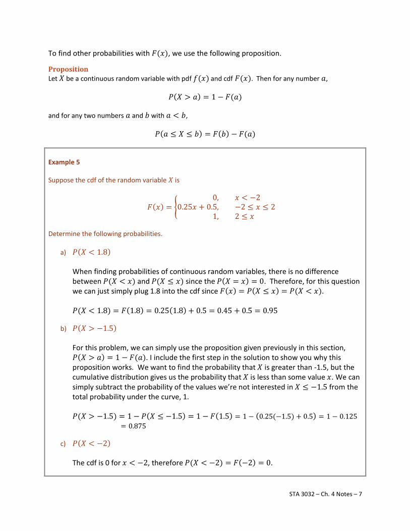
𝑃(𝑎 ≤ 𝑋 ≤ 𝑏) = 𝐹(𝑏) − 𝐹(𝑎) Example 5 Suppose the cdf of the random variable 𝑋 is

𝐹(𝑥) = �0, 𝑥 < −2

0.25𝑥 + 0.5, −2 ≤ 𝑥 ≤ 21, 2 ≤ 𝑥

Determine the following probabilities.

a) 𝑃(𝑋 < 1.8)

When finding probabilities of continuous random variables, there is no difference between 𝑃(𝑋 < 𝑥) and 𝑃(𝑋 ≤ 𝑥) since the 𝑃(𝑋 = 𝑥) = 0. Therefore, for this question we can just simply plug 1.8 into the cdf since 𝐹(𝑥) = 𝑃(𝑋 ≤ 𝑥) = 𝑃(𝑋 < 𝑥). 𝑃(𝑋 < 1.8) = 𝐹(1.8) = 0.25(1.8) + 0.5 = 0.45 + 0.5 = 0.95

b) 𝑃(𝑋 > −1.5)

For this problem, we can simply use the proposition given previously in this section, 𝑃(𝑋 > 𝑎) = 1 − 𝐹(𝑎). I include the first step in the solution to show you why this proposition works. We want to find the probability that 𝑋 is greater than -1.5, but the cumulative distribution gives us the probability that 𝑋 is less than some value 𝑥. We can simply subtract the probability of the values we’re not interested in 𝑋 ≤ −1.5 from the total probability under the curve, 1. 𝑃(𝑋 > −1.5) = 1 − 𝑃(𝑋 ≤ −1.5) = 1 − 𝐹(1.5) = 1 − (0.25(−1.5) + 0.5) = 1 − 0.125

= 0.875

c) 𝑃(𝑋 < −2) The cdf is 0 for 𝑥 < −2, therefore 𝑃(𝑋 < −2) = 𝐹(−2) = 0.

STA 3032 – Ch. 4 Notes – 7

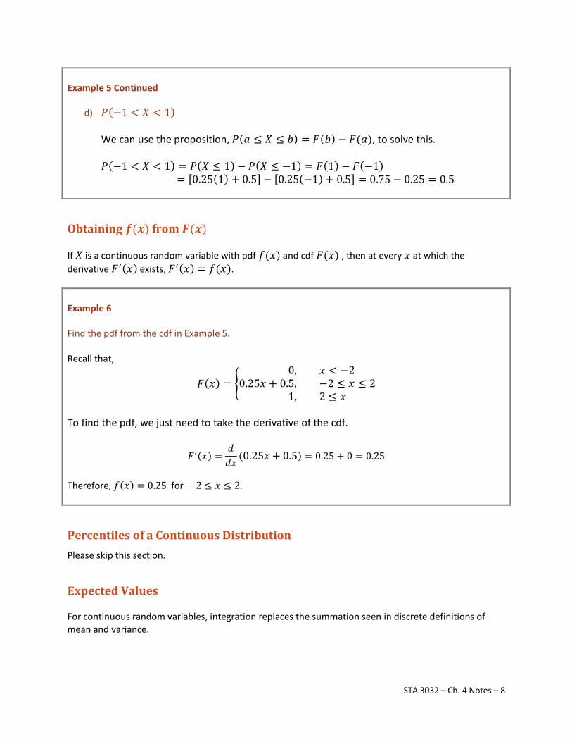
Example 5 Continued

d) 𝑃(−1 < 𝑋 < 1)

We can use the proposition, 𝑃(𝑎 ≤ 𝑋 ≤ 𝑏) = 𝐹(𝑏) − 𝐹(𝑎), to solve this.

𝑃(−1 < 𝑋 < 1) = 𝑃(𝑋 ≤ 1) − 𝑃(𝑋 ≤ −1) = 𝐹(1) − 𝐹(−1)

= [0.25(1) + 0.5] − [0.25(−1) + 0.5] = 0.75 − 0.25 = 0.5

Obtaining 𝒇(𝒙) from 𝑭(𝒙) If 𝑋 is a continuous random variable with pdf 𝑓(𝑥) and cdf 𝐹(𝑥) , then at every 𝑥 at which the derivative 𝐹′(𝑥) exists, 𝐹′(𝑥) = 𝑓(𝑥). Example 6 Find the pdf from the cdf in Example 5. Recall that,

𝐹(𝑥) = �0, 𝑥 < −2

0.25𝑥 + 0.5, −2 ≤ 𝑥 ≤ 21, 2 ≤ 𝑥

To find the pdf, we just need to take the derivative of the cdf.

𝐹′(𝑥) =𝑑𝑑𝑥

(0.25𝑥+ 0.5) = 0.25 + 0 = 0.25

Therefore, 𝑓(𝑥) = 0.25 for −2 ≤ 𝑥 ≤ 2.

Percentiles of a Continuous Distribution

Please skip this section.

Expected Values For continuous random variables, integration replaces the summation seen in discrete definitions of mean and variance.

STA 3032 – Ch. 4 Notes – 8

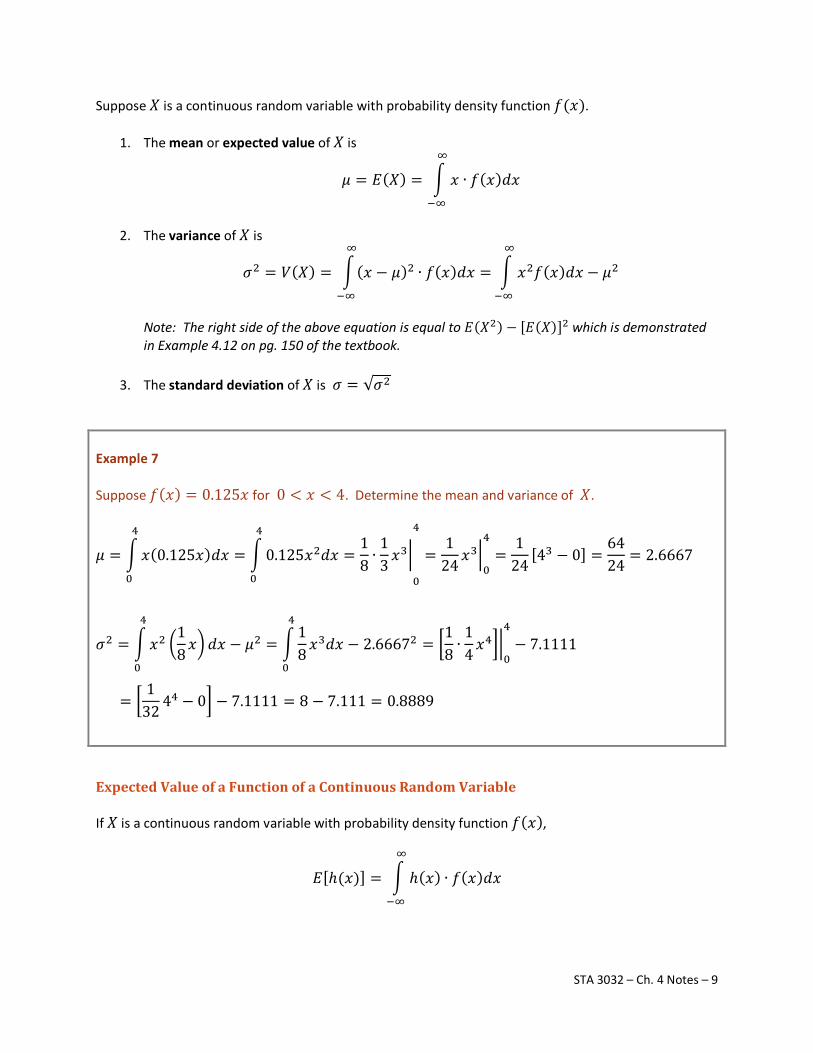
Suppose 𝑋 is a continuous random variable with probability density function 𝑓(𝑥).

1. The mean or expected value of 𝑋 is

𝜇 = 𝐸(𝑋) = � 𝑥 ∙ 𝑓(𝑥)𝑑𝑥∞

−∞

2. The variance of 𝑋 is

𝜎2 = 𝑉(𝑋) = �(𝑥 − 𝜇)2 ∙ 𝑓(𝑥)𝑑𝑥 =∞

−∞

� 𝑥2𝑓(𝑥)𝑑𝑥 − 𝜇2∞

−∞

Note: The right side of the above equation is equal to 𝐸(𝑋2) − [𝐸(𝑋)]2 which is demonstrated in Example 4.12 on pg. 150 of the textbook.

3. The standard deviation of 𝑋 is 𝜎 = √𝜎2

Example 7 Suppose 𝑓(𝑥) = 0.125𝑥 for 0 < 𝑥 < 4. Determine the mean and variance of 𝑋.

𝜇 = �𝑥(0.125𝑥)𝑑𝑥 = � 0.125𝑥2𝑑𝑥4

0

=18 ∙

13 𝑥

3�4

0 0

4

=1

24 𝑥3�0

4

=1

24[43 − 0] =

6424 = 2.6667

𝜎2 = �𝑥2 �18𝑥� 𝑑𝑥

4

0

− 𝜇2 = �18 𝑥

3𝑑𝑥4

0

− 2.66672 = �18 ∙

14 𝑥

4��0

4

− 7.1111

= �1

32 44 − 0� − 7.1111 = 8 − 7.111 = 0.8889

Expected Value of a Function of a Continuous Random Variable If 𝑋 is a continuous random variable with probability density function 𝑓(𝑥),

𝐸[ℎ(𝑥)] = � ℎ(𝑥) ∙ 𝑓(𝑥)𝑑𝑥∞

−∞

STA 3032 – Ch. 4 Notes – 9

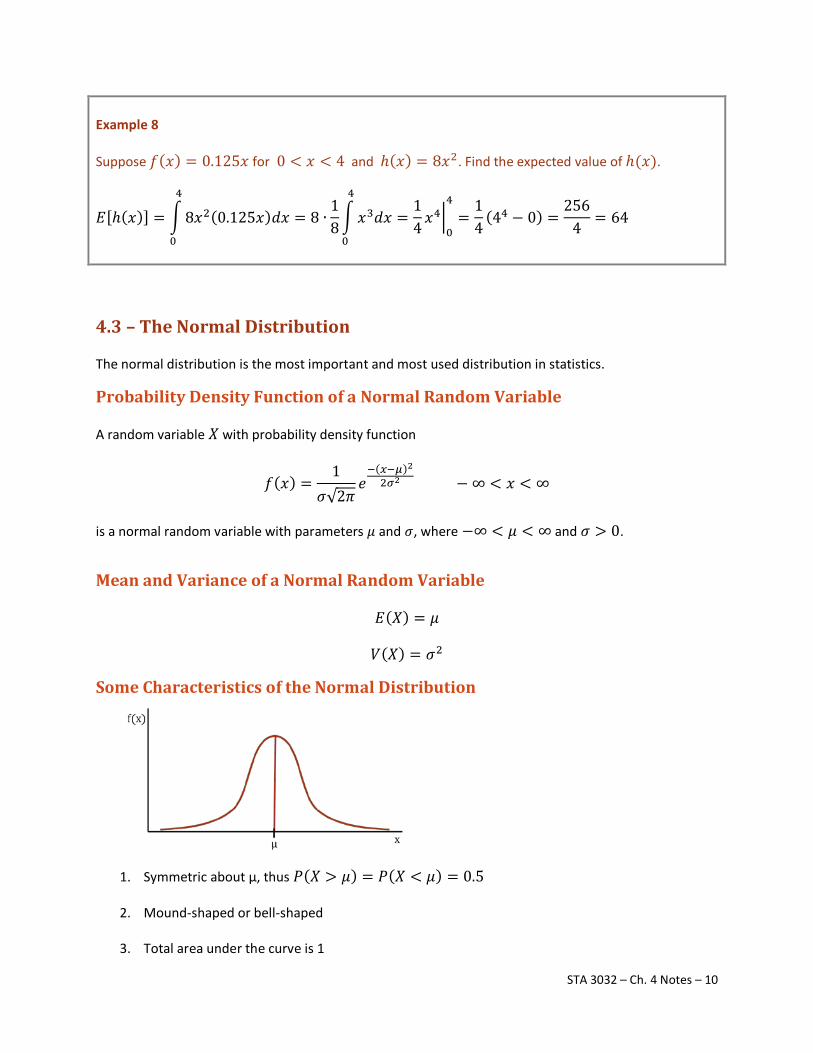
Example 8 Suppose 𝑓(𝑥) = 0.125𝑥 for 0 < 𝑥 < 4 and ℎ(𝑥) = 8𝑥2. Find the expected value of ℎ(𝑥).

𝐸[ℎ(𝑥)] = �8𝑥2(0.125𝑥)𝑑𝑥 = 8 ∙18�𝑥3𝑑𝑥4

0

4

0

=14 𝑥

4�0

4

=14

(44 − 0) =256

4 = 64

4.3 – The Normal Distribution The normal distribution is the most important and most used distribution in statistics.

Probability Density Function of a Normal Random Variable A random variable 𝑋 with probability density function

𝑓(𝑥) =1

𝜎√2𝜋𝑒−(𝑥−𝜇)22𝜎2 −∞ < 𝑥 < ∞

is a normal random variable with parameters 𝜇 and 𝜎, where −∞ < 𝜇 < ∞ and 𝜎 > 0.

Mean and Variance of a Normal Random Variable

𝐸(𝑋) = 𝜇

𝑉(𝑋) = 𝜎2

Some Characteristics of the Normal Distribution

1. Symmetric about µ, thus 𝑃(𝑋 > 𝜇) = 𝑃(𝑋 < 𝜇) = 0.5

2. Mound-shaped or bell-shaped

3. Total area under the curve is 1

STA 3032 – Ch. 4 Notes – 10

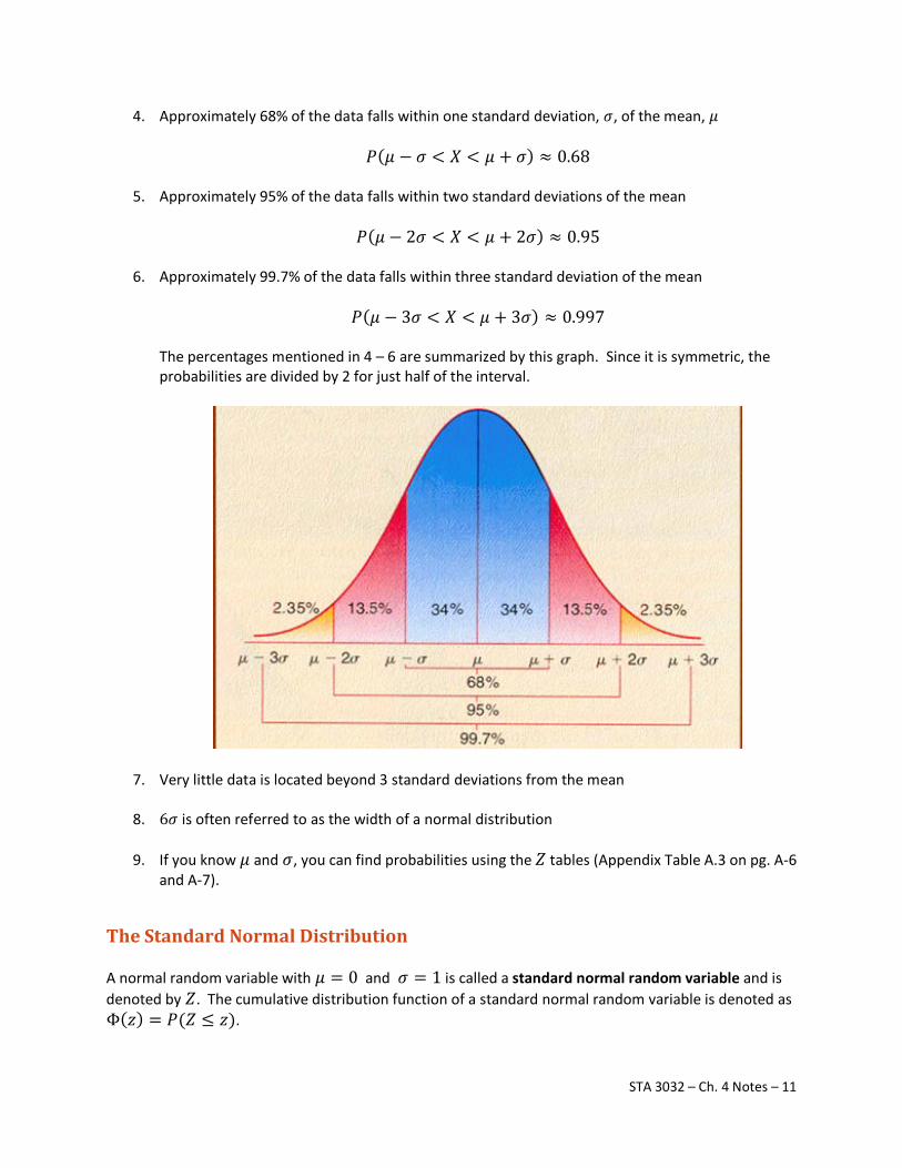
4. Approximately 68% of the data falls within one standard deviation, 𝜎, of the mean, 𝜇

𝑃(𝜇 − 𝜎 < 𝑋 < 𝜇 + 𝜎) ≈ 0.68

5. Approximately 95% of the data falls within two standard deviations of the mean

𝑃(𝜇 − 2𝜎 < 𝑋 < 𝜇 + 2𝜎) ≈ 0.95

6. Approximately 99.7% of the data falls within three standard deviation of the mean

𝑃(𝜇 − 3𝜎 < 𝑋 < 𝜇 + 3𝜎) ≈ 0.997 The percentages mentioned in 4 – 6 are summarized by this graph. Since it is symmetric, the probabilities are divided by 2 for just half of the interval.

7. Very little data is located beyond 3 standard deviations from the mean

8. 6𝜎 is often referred to as the width of a normal distribution

9. If you know 𝜇 and 𝜎, you can find probabilities using the 𝑍 tables (Appendix Table A.3 on pg. A-6 and A-7).

The Standard Normal Distribution A normal random variable with 𝜇 = 0 and 𝜎 = 1 is called a standard normal random variable and is denoted by 𝑍. The cumulative distribution function of a standard normal random variable is denoted as Φ(𝑧) = 𝑃(𝑍 ≤ 𝑧).

STA 3032 – Ch. 4 Notes – 11

Appendix Table A.3 on pg. A-6 and A-7 provides the cumulative probabilities for a standard normal random variable. I’ll refer to this table as the 𝑍 table.

How to Use the Z Table The table on pages A-6 and A-7 gives the cumulative probability of 𝑍, 𝑃(𝑍 ≤ 𝑧), for −3.49 ≤ 𝑧 ≤3.49.

1. Find the first two digits of 𝑧 in the left column and place left finger there 2. Find the third digit of 𝑧 at the top of the table and place right finger there 3. Move your right finger down until it’s at the same row as your left finger, this is the cumulative

probability for that value of 𝑧 Example 9 Use Appendix Table A.3 to determine the following probabilities for the standard normal random variable Z.

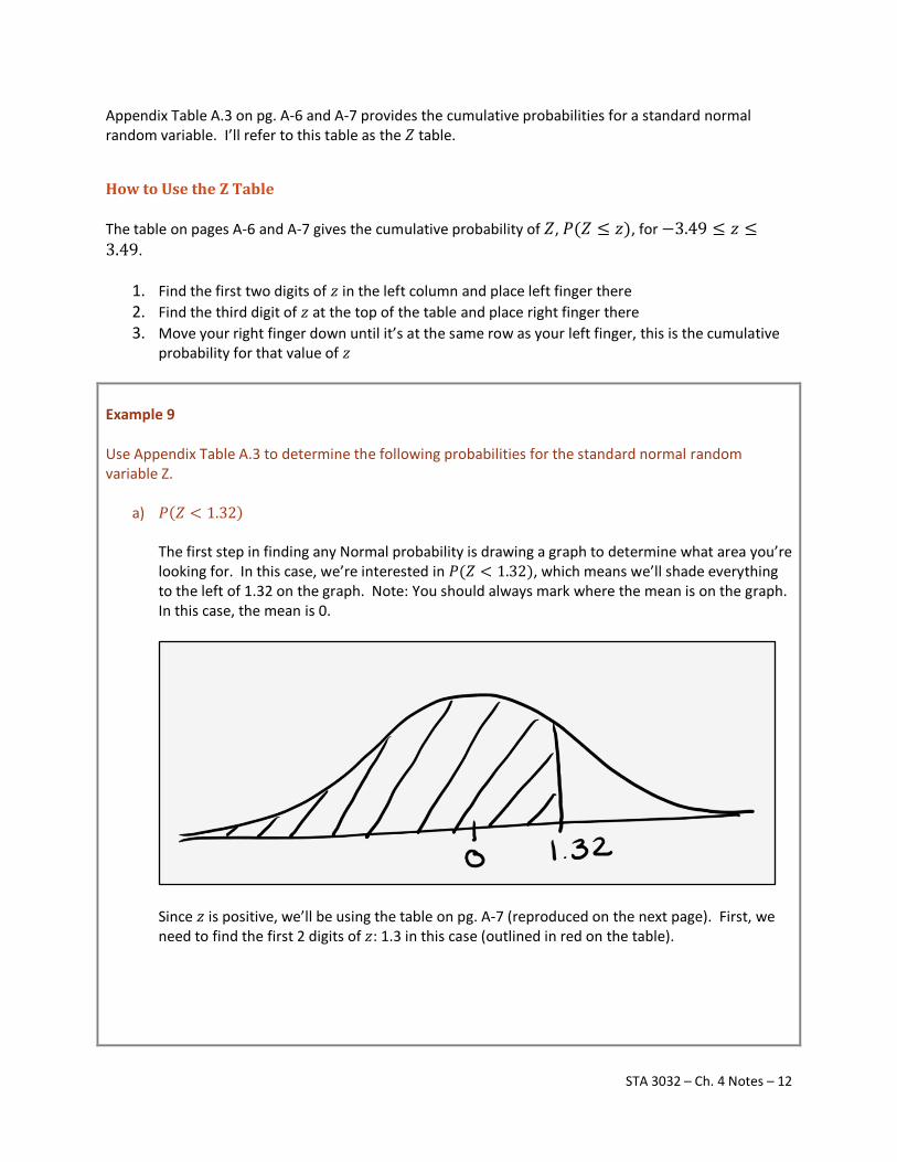
a) 𝑃(𝑍 < 1.32)

The first step in finding any Normal probability is drawing a graph to determine what area you’re looking for. In this case, we’re interested in 𝑃(𝑍 < 1.32), which means we’ll shade everything to the left of 1.32 on the graph. Note: You should always mark where the mean is on the graph. In this case, the mean is 0.

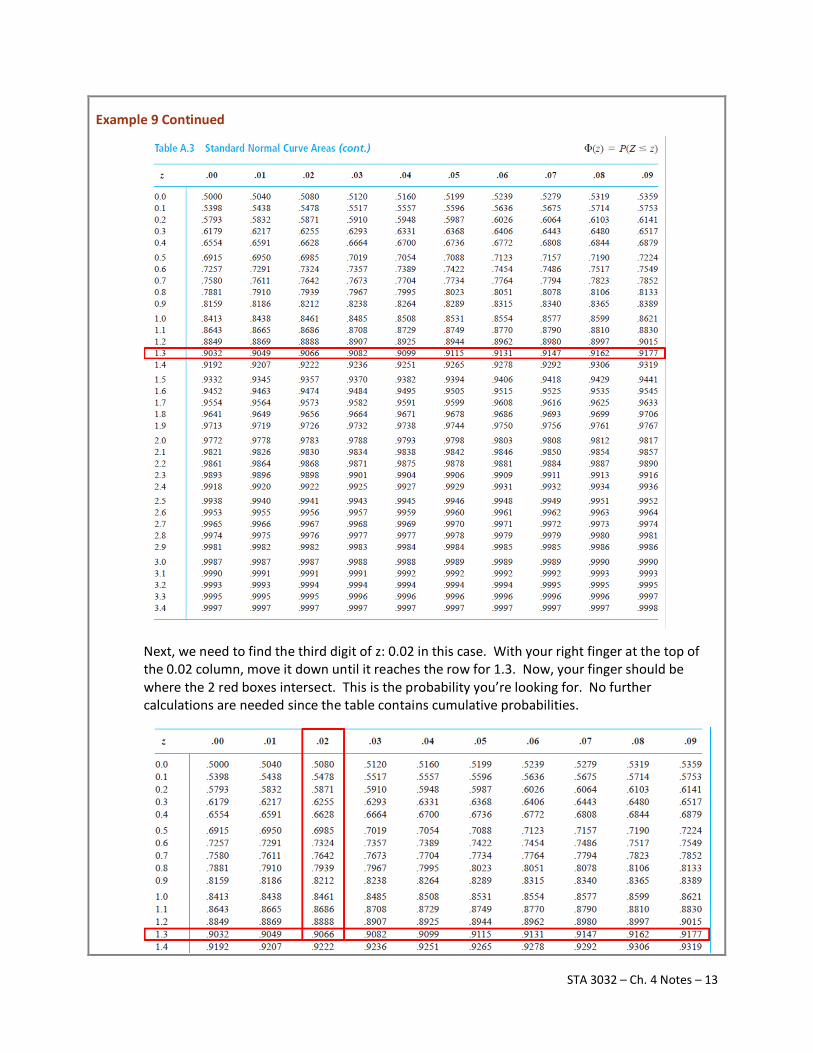
Since 𝑧 is positive, we’ll be using the table on pg. A-7 (reproduced on the next page). First, we need to find the first 2 digits of 𝑧: 1.3 in this case (outlined in red on the table).

STA 3032 – Ch. 4 Notes – 12

Example 9 Continued

Next, we need to find the third digit of z: 0.02 in this case. With your right finger at the top of the 0.02 column, move it down until it reaches the row for 1.3. Now, your finger should be where the 2 red boxes intersect. This is the probability you’re looking for. No further calculations are needed since the table contains cumulative probabilities.

STA 3032 – Ch. 4 Notes – 13

Example 9 Continued

Now we can label the shaded area of the graph with the probability we found.

𝑃(𝑍 < 1.32) = .9066

Note: You should never round probabilities found in the 𝑍 tables even if the directions say to round to a lesser number of decimal places.

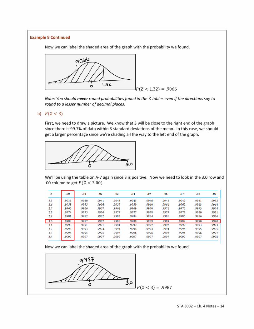
b) 𝑃(𝑍 < 3) First, we need to draw a picture. We know that 3 will be close to the right end of the graph since there is 99.7% of data within 3 standard deviations of the mean. In this case, we should get a larger percentage since we’re shading all the way to the left end of the graph.

We’ll be using the table on A-7 again since 3 is positive. Now we need to look in the 3.0 row and .00 column to get 𝑃(𝑍 < 3.00).

Now we can label the shaded area of the graph with the probability we found.

𝑃(𝑍 < 3) = .9987

STA 3032 – Ch. 4 Notes – 14

Example 9 Continued

c) 𝑃(𝑍 > 1.45) Note: The book writes this as 𝑃(1.45 ≤ 𝑍), but I will use this equivalent notation.

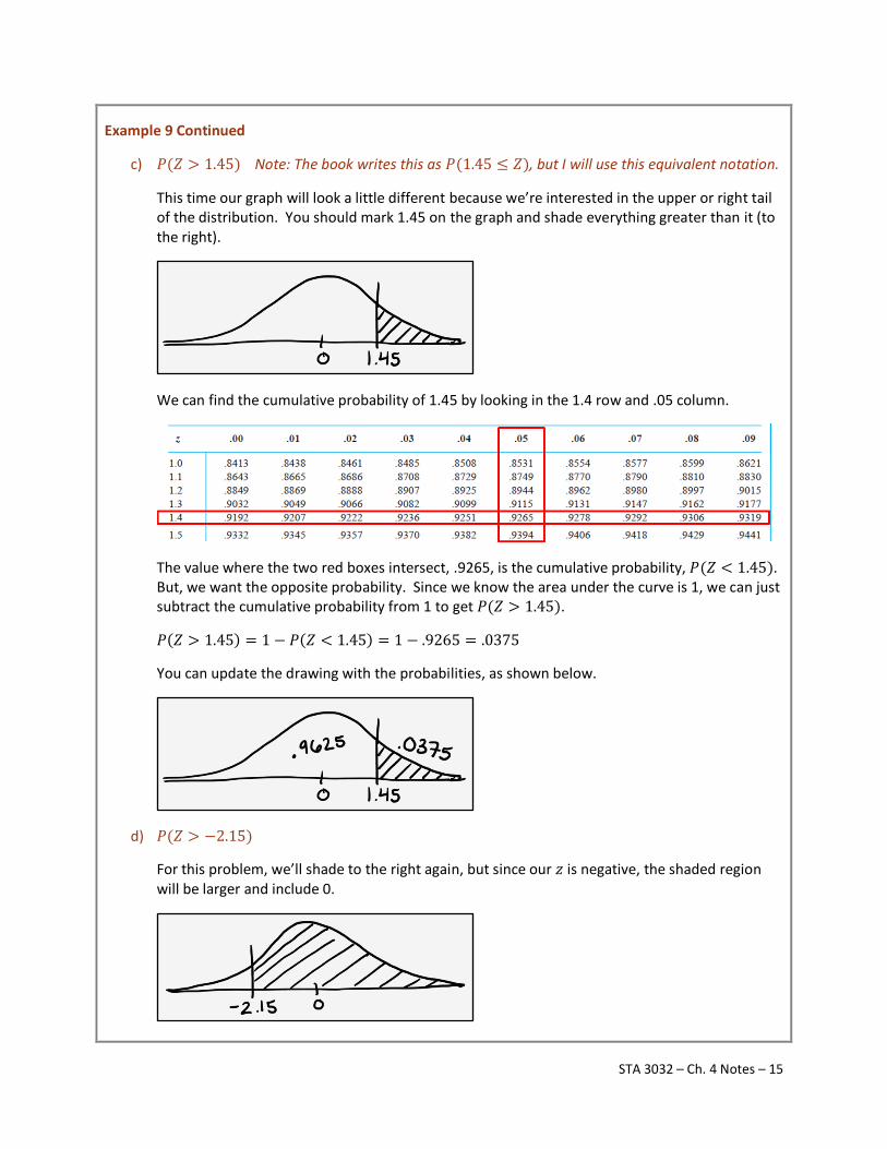
This time our graph will look a little different because we’re interested in the upper or right tail of the distribution. You should mark 1.45 on the graph and shade everything greater than it (to the right).

We can find the cumulative probability of 1.45 by looking in the 1.4 row and .05 column.

The value where the two red boxes intersect, .9265, is the cumulative probability, 𝑃(𝑍 < 1.45). But, we want the opposite probability. Since we know the area under the curve is 1, we can just subtract the cumulative probability from 1 to get 𝑃(𝑍 > 1.45). 𝑃(𝑍 > 1.45) = 1 − 𝑃(𝑍 < 1.45) = 1 − .9265 = .0375

You can update the drawing with the probabilities, as shown below.

d) 𝑃(𝑍 > −2.15)

For this problem, we’ll shade to the right again, but since our 𝑧 is negative, the shaded region will be larger and include 0.

STA 3032 – Ch. 4 Notes – 15

Example 9 Continued

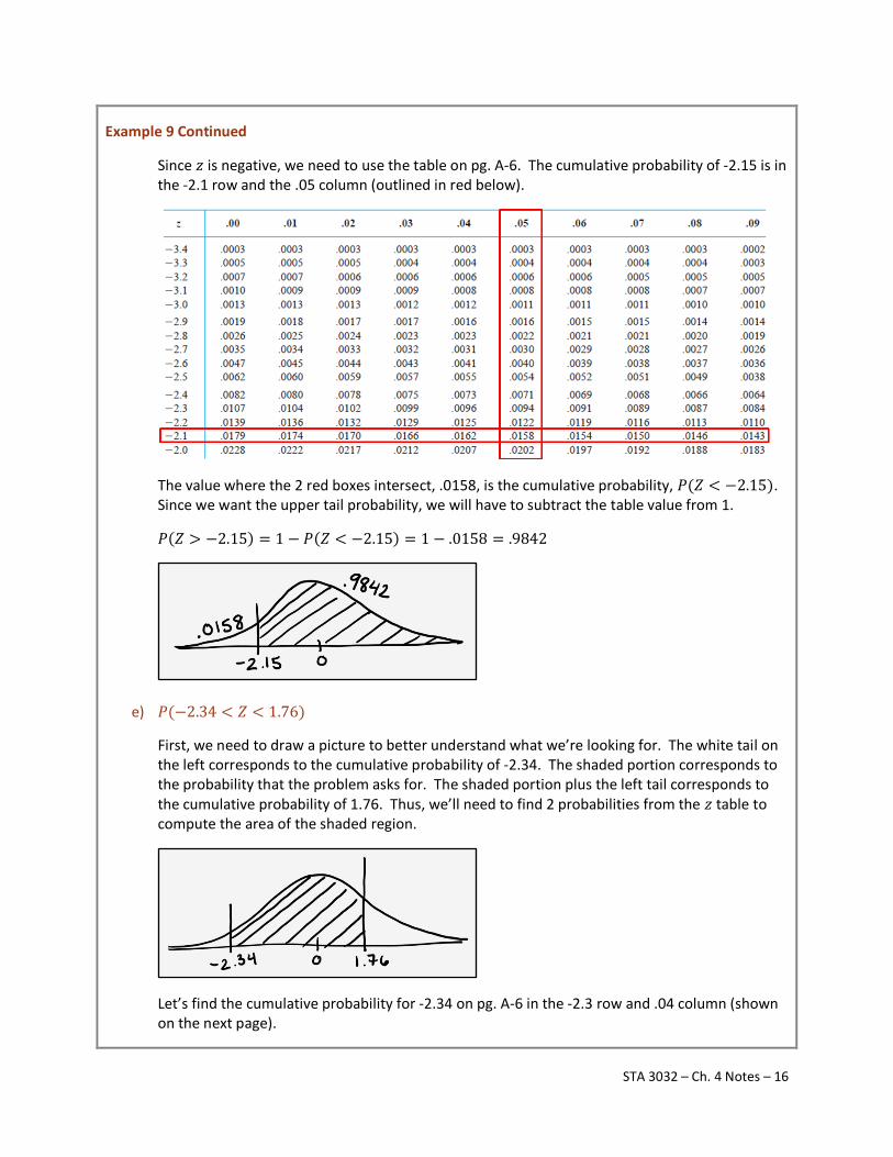
Since 𝑧 is negative, we need to use the table on pg. A-6. The cumulative probability of -2.15 is in the -2.1 row and the .05 column (outlined in red below).

The value where the 2 red boxes intersect, .0158, is the cumulative probability, 𝑃(𝑍 < −2.15). Since we want the upper tail probability, we will have to subtract the table value from 1.

𝑃(𝑍 > −2.15) = 1 − 𝑃(𝑍 < −2.15) = 1 − .0158 = .9842

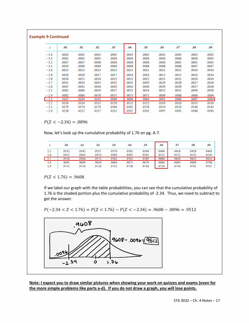
e) 𝑃(−2.34 < 𝑍 < 1.76)

First, we need to draw a picture to better understand what we’re looking for. The white tail on the left corresponds to the cumulative probability of -2.34. The shaded portion corresponds to the probability that the problem asks for. The shaded portion plus the left tail corresponds to the cumulative probability of 1.76. Thus, we’ll need to find 2 probabilities from the 𝑧 table to compute the area of the shaded region.

Let’s find the cumulative probability for -2.34 on pg. A-6 in the -2.3 row and .04 column (shown on the next page).

STA 3032 – Ch. 4 Notes – 16

Example 9 Continued

𝑃(𝑍 < −2.34) = .0096 Now, let’s look up the cumulative probability of 1.76 on pg. A-7.

𝑃(𝑍 < 1.76) = .9608

If we label our graph with the table probabilities, you can see that the cumulative probability of 1.76 is the shaded portion plus the cumulative probability of -2.34. Thus, we need to subtract to get the answer. 𝑃(−2.34 < 𝑍 < 1.76) = 𝑃(𝑍 < 1.76) − 𝑃(𝑍 < −2.34) = .9608 − .0096 = .9512

Note: I expect you to draw similar pictures when showing your work on quizzes and exams (even for the more simple problems like parts a-d). If you do not draw a graph, you will lose points.

STA 3032 – Ch. 4 Notes – 17

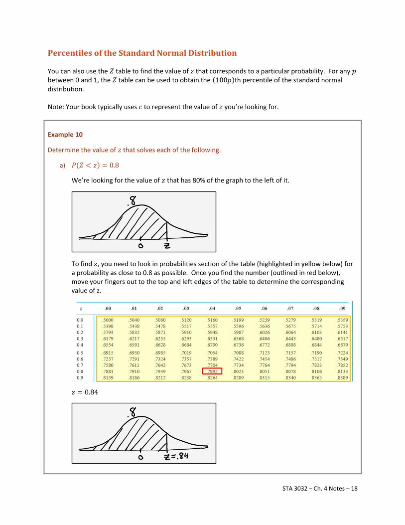
Percentiles of the Standard Normal Distribution You can also use the 𝑍 table to find the value of 𝑧 that corresponds to a particular probability. For any 𝑝 between 0 and 1, the 𝑍 table can be used to obtain the (100𝑝)th percentile of the standard normal distribution. Note: Your book typically uses 𝑐 to represent the value of 𝑧 you’re looking for. Example 10

Determine the value of 𝑧 that solves each of the following.

a) 𝑃(𝑍 < 𝑧) = 0.8

We’re looking for the value of 𝑧 that has 80% of the graph to the left of it.

To find 𝑧, you need to look in probabilities section of the table (highlighted in yellow below) for a probability as close to 0.8 as possible. Once you find the number (outlined in red below), move your fingers out to the top and left edges of the table to determine the corresponding value of z.

𝑧 = 0.84

STA 3032 – Ch. 4 Notes – 18

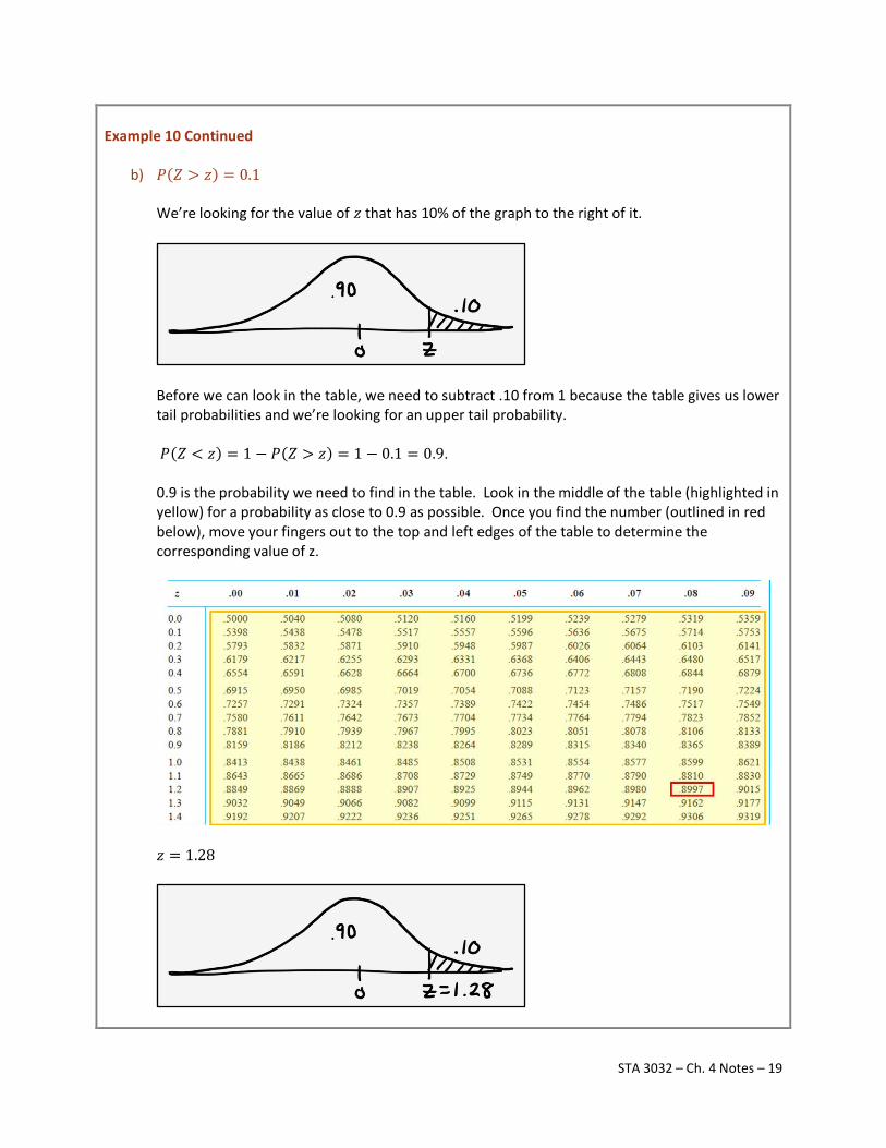
Example 10 Continued

b) 𝑃(𝑍 > 𝑧) = 0.1 We’re looking for the value of 𝑧 that has 10% of the graph to the right of it.

Before we can look in the table, we need to subtract .10 from 1 because the table gives us lower tail probabilities and we’re looking for an upper tail probability. 𝑃(𝑍 < 𝑧) = 1 − 𝑃(𝑍 > 𝑧) = 1 − 0.1 = 0.9. 0.9 is the probability we need to find in the table. Look in the middle of the table (highlighted in yellow) for a probability as close to 0.9 as possible. Once you find the number (outlined in red below), move your fingers out to the top and left edges of the table to determine the corresponding value of z.

𝑧 = 1.28

STA 3032 – Ch. 4 Notes – 19

𝒛𝜶 Notation for 𝒛 Critical Values Please read this section in the book on pg. 156.

Nonstandard Normal Distributions If 𝑋 is a normal random variable with 𝐸(𝑋) = 𝜇 and 𝑉(𝑋) = 𝜎2, then the random variable

𝑍 =𝑥 − 𝜇𝜎

is a normal random variable with 𝐸(𝑍) = 0 and 𝑉(𝑍) = 1. Thus, it is a standard normal random variable. The above formula is called a z-score. It is the number of standard deviations that an observation, 𝑥, is from the mean, 𝜇. If a z-score is negative, then the observation is less than the mean. If a z-score is positive, the observation is greater than the mean. If a z-score equals zero, then the observation is equal to the mean. We standardize normal random variables because then we can use the 𝑍 table to find probabilities, which is much easier than the alternative: integration. Example 11 Let 𝑋 be normally distributed with a mean of 600 and standard deviation of 100. Find the z-score for 𝑥 = 625.

𝑧 =𝑥 − 𝜇𝜎

=625 − 600

100=

25100

= 0.25

Standardizing to Calculate a Probability Suppose 𝑋 is a normal random variable with mean 𝜇 and variance 𝜎2. Then,

𝑃(𝑋 ≤ 𝑥) = 𝑃 �𝑋 − 𝜇𝜎 ≤

𝑥 − 𝜇𝜎

� = 𝑃(𝑍 ≤ 𝑧)

where 𝑍 is a standard normal random variable, and 𝑧 = 𝑥−𝜇

𝜎 is the z-score obtained by standardizing 𝑋.

The probability is obtained by using the 𝑍 table.

STA 3032 – Ch. 4 Notes – 20

Example 12

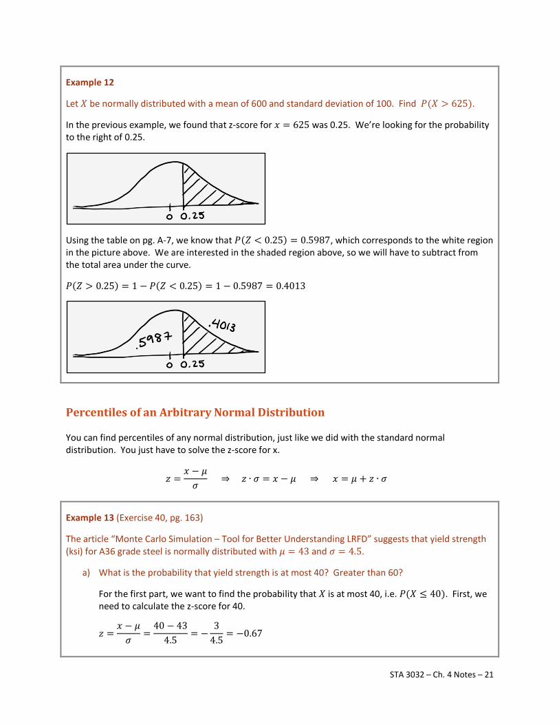
Let 𝑋 be normally distributed with a mean of 600 and standard deviation of 100. Find 𝑃(𝑋 > 625).

In the previous example, we found that z-score for 𝑥 = 625 was 0.25. We’re looking for the probability to the right of 0.25.

Using the table on pg. A-7, we know that 𝑃(𝑍 < 0.25) = 0.5987, which corresponds to the white region in the picture above. We are interested in the shaded region above, so we will have to subtract from the total area under the curve.

𝑃(𝑍 > 0.25) = 1 − 𝑃(𝑍 < 0.25) = 1 − 0.5987 = 0.4013

Percentiles of an Arbitrary Normal Distribution You can find percentiles of any normal distribution, just like we did with the standard normal distribution. You just have to solve the z-score for x.

𝑧 =𝑥 − 𝜇𝜎

⇒ 𝑧 ∙ 𝜎 = 𝑥 − 𝜇 ⇒ 𝑥 = 𝜇 + 𝑧 ∙ 𝜎 Example 13 (Exercise 40, pg. 163) The article “Monte Carlo Simulation – Tool for Better Understanding LRFD” suggests that yield strength (ksi) for A36 grade steel is normally distributed with 𝜇 = 43 and 𝜎 = 4.5.

a) What is the probability that yield strength is at most 40? Greater than 60?

For the first part, we want to find the probability that 𝑋 is at most 40, i.e. 𝑃(𝑋 ≤ 40). First, we need to calculate the z-score for 40.

𝑧 =𝑥 − 𝜇𝜎

=40 − 43

4.5= −

34.5

= −0.67

STA 3032 – Ch. 4 Notes – 21

Example 13 Continued

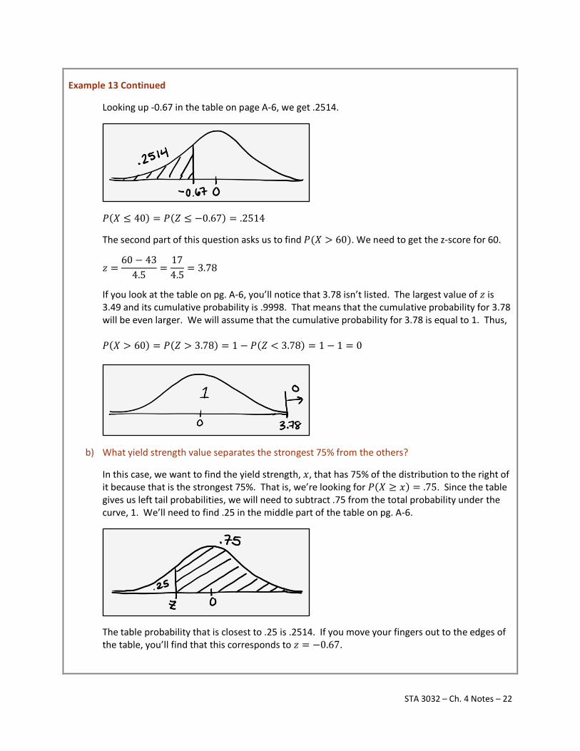
Looking up -0.67 in the table on page A-6, we get .2514.

𝑃(𝑋 ≤ 40) = 𝑃(𝑍 ≤ −0.67) = .2514 The second part of this question asks us to find 𝑃(𝑋 > 60). We need to get the z-score for 60.

𝑧 =60 − 43

4.5=

174.5

= 3.78

If you look at the table on pg. A-6, you’ll notice that 3.78 isn’t listed. The largest value of 𝑧 is 3.49 and its cumulative probability is .9998. That means that the cumulative probability for 3.78 will be even larger. We will assume that the cumulative probability for 3.78 is equal to 1. Thus, 𝑃(𝑋 > 60) = 𝑃(𝑍 > 3.78) = 1 − 𝑃(𝑍 < 3.78) = 1 − 1 = 0

b) What yield strength value separates the strongest 75% from the others?

In this case, we want to find the yield strength, 𝑥, that has 75% of the distribution to the right of it because that is the strongest 75%. That is, we’re looking for 𝑃(𝑋 ≥ 𝑥) = .75. Since the table gives us left tail probabilities, we will need to subtract .75 from the total probability under the curve, 1. We’ll need to find .25 in the middle part of the table on pg. A-6.

The table probability that is closest to .25 is .2514. If you move your fingers out to the edges of the table, you’ll find that this corresponds to 𝑧 = −0.67.

STA 3032 – Ch. 4 Notes – 22

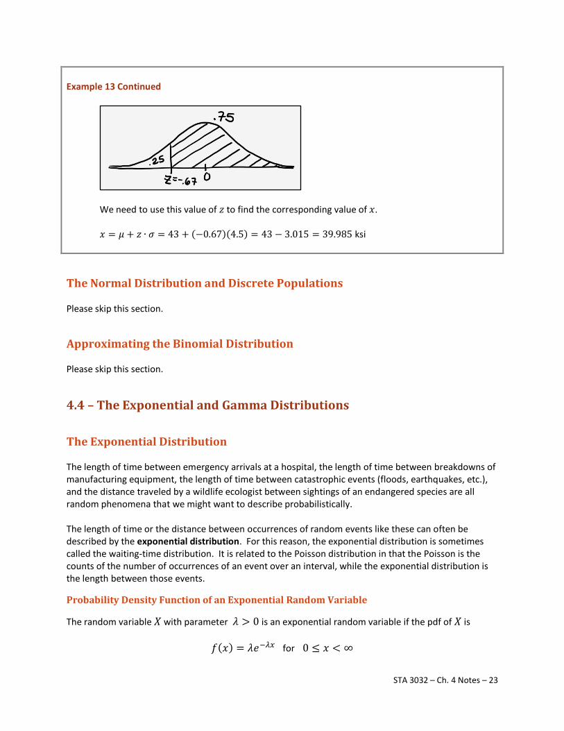
Example 13 Continued

We need to use this value of 𝑧 to find the corresponding value of 𝑥. 𝑥 = 𝜇 + 𝑧 ∙ 𝜎 = 43 + (−0.67)(4.5) = 43 − 3.015 = 39.985 ksi

The Normal Distribution and Discrete Populations Please skip this section.

Approximating the Binomial Distribution Please skip this section.

4.4 – The Exponential and Gamma Distributions

The Exponential Distribution The length of time between emergency arrivals at a hospital, the length of time between breakdowns of manufacturing equipment, the length of time between catastrophic events (floods, earthquakes, etc.), and the distance traveled by a wildlife ecologist between sightings of an endangered species are all random phenomena that we might want to describe probabilistically. The length of time or the distance between occurrences of random events like these can often be described by the exponential distribution. For this reason, the exponential distribution is sometimes called the waiting-time distribution. It is related to the Poisson distribution in that the Poisson is the counts of the number of occurrences of an event over an interval, while the exponential distribution is the length between those events.

Probability Density Function of an Exponential Random Variable

The random variable 𝑋 with parameter 𝜆 > 0 is an exponential random variable if the pdf of 𝑋 is

𝑓(𝑥) = 𝜆𝑒−𝜆𝑥 for 0 ≤ 𝑥 < ∞

STA 3032 – Ch. 4 Notes – 23

Mean and Variance of an Exponential Random Variable If the random variable 𝑋 has an exponential distribution with parameter 𝜆,

𝜇 = 𝐸(𝑋) =1𝜆

𝜎2 = 𝑉(𝑋) =1𝜆2

Cumulative Density Function of an Exponential Random Variable If the random variable 𝑋 has an exponential distribution with parameter 𝜆, the the cdf of 𝑋 is

𝐹(𝑥) = 1 − 𝑒−𝜆𝑥 for 0 ≤ 𝑥 < ∞ Note: You should be able to use the cdf to answer most Exponential questions. This will allow you to avoid integrating the pdf.

Example 14 The distance between major cracks in a highway follows an exponential distribution with a mean of 5 miles.

a) What is the probability that there are no major cracks in a 10-mile stretch of the highway?

First, let’s define an exponential random variable 𝑋 = distance between major cracks. Since 𝜇 = 5 = 1

𝜆, solving for λ, we get 𝜆 = 1

5= 0.2.

If we want to find the probability that there are no major cracks in a 10-mile stretch of a roadway, that means the distance between cracks must be larger than 10 miles. Therefore, we are looking for the probability that 𝑋 is greater than 10. We can use the cdf to find this answer by subtracting 𝐹(10) from the total probability.

𝑃(𝑋 > 10) = 1 − 𝑃(𝑋 ≤ 10) = 1 − 𝐹(10) = 1 − �1 − 𝑒−0.2(10)� = −𝑒−2 = 0.1353

b) What is the standard deviation of the distance between major cracks?

𝑉(𝑋) =1

0.22=

10.04

= 25 𝜎 = √25 = 5

c) What is the probability that the first major crack occurs between 12 and 15 miles of the start of

inspection?

𝑃(12 < 𝑋 < 15) = 𝑃(𝑋 ≤ 15) − 𝑃(𝑋 ≤ 12) = 𝐹(15) − 𝐹(12)

= �1 − 𝑒−0.2(15)� − �1− 𝑒−0.2(12)� = (1− 𝑒−3) − (1− 𝑒−2.4)

= 1 − 𝑒−3 − 1 + 𝑒−2.4 = −𝑒−3 + 𝑒−2.4 = 0.0409

STA 3032 – Ch. 4 Notes – 24

The Gamma Distribution Please skip this section.

The Chi-Squared Distribution Please skip this section. We may cover this distribution later in the semester.

4.5 – Other Continuous Distributions Please skip this section.

4.6 – Probability Plots Please skip this section. We may cover it later in the semester.

STA 3032 – Ch. 4 Notes – 25