
402131
59
Dynamic Neural Networks for Model-Free Control and Identification Guest Editors: Alex Poznyak, Isaac Chairez, Haibo He, and Wen Yu Journal of Control Science and Engineering
Transcript of 402131

Dynamic Neural Networks for Model-Free Control and Identification
Guest Editors: Alex Poznyak, Isaac Chairez, Haibo He, and Wen Yu
Journal of Control Science and Engineering

Dynamic Neural Networks for Model-FreeControl and Identification

Journal of Control Science and Engineering
Dynamic Neural Networks for Model-FreeControl and Identification
Guest Editors: Alex Poznyak, Isaac Chairez, Haibo He,and Wen Yu

Copyright © 2012 Hindawi Publishing Corporation. All rights reserved.
This is a special issue published in “Journal of Control Science and Engineering.” All articles are open access articles distributed underthe Creative Commons Attribution License, which permits unrestricted use, distribution, and reproduction in any medium, providedthe original work is properly cited.

Editorial Board
Edwin K. P. Chong, USARicardo Dunia, USANicola Elia, USAPeilin Fu, USABijoy K. Ghosh, USAF. Gordillo, SpainShinji Hara, Japan
Seul Jung, Republic of KoreaVladimir Kharitonov, RussiaJames Lam, Hong KongDerong Liu, ChinaTomas McKelvey, SwedenSilviu-Iulian Niculescu, FranceYoshito Ohta, Japan
Yang Shi, CanadaZoltan Szabo, HungaryOnur Toker, TurkeyXiaofan Wang, ChinaJianliang Wang, SingaporeWen Yu, MexicoMohamed A. Zribi, Kuwait

Contents
Dynamic Neural Networks for Model-Free Control and Identification, Alex Poznyak, Isaac Chairez,Haibo He, and Wen YuVolume 2012, Article ID 916340, 2 pages
Experimental Studies of Neural Network Control for One-Wheel Mobile Robot, P. K. Kim and S. JungVolume 2012, Article ID 194397, 12 pages
Robust Adaptive Control via Neural Linearization and Compensation, Roberto Carmona Rodrıguez andWen YuVolume 2012, Article ID 867178, 9 pages
Dynamics Model Abstraction Scheme Using Radial Basis Functions, Silvia Tolu, Mauricio Vanegas,Rodrigo Agıs, Richard Carrillo, and Antonio CanasVolume 2012, Article ID 761019, 11 pages
An Output-Recurrent-Neural-Network-Based Iterative Learning Control for Unknown NonlinearDynamic Plants, Ying-Chung Wang and Chiang-Ju ChienVolume 2012, Article ID 545731, 9 pages
3D Nonparametric Neural Identification, Rita Q. Fuentes, Isaac Chairez, Alexander Poznyak,and Tatyana PoznyakVolume 2012, Article ID 618403, 10 pages

Hindawi Publishing CorporationJournal of Control Science and EngineeringVolume 2012, Article ID 916340, 2 pagesdoi:10.1155/2012/916340
Editorial
Dynamic Neural Networks for Model-FreeControl and Identification
Alex Poznyak,1 Isaac Chairez,2 Haibo He,3 and Wen Yu1
1 Departamento de Control Automatico, Centro de Investigacion y de Estudios Avanzados, 07360 Mexico City, DF, Mexico2 UPIBI, Biotechnology Department, National Polytecnical Institute (IPN), 07738 Mexico City, DF, Mexico3 Department of Electrical, Computer, and Biomedical Engineering, University of Rhode Island, Kingston, RI 02881, USA
Correspondence should be addressed to Alex Poznyak, [email protected]
Received 17 December 2012; Accepted 17 December 2012
Copyright © 2012 Alex Poznyak et al. This is an open access article distributed under the Creative Commons Attribution License,which permits unrestricted use, distribution, and reproduction in any medium, provided the original work is properly cited.
Neural networks have been used to solve a broad diversity ofproblems on different scientific and technological disciplines.Particularly, control and identification of uncertain systemshave received attention since many years ago by the naturalinterest to solve problem such as automatic regulation ortracking of systems having a high degree of vagueness ontheir formal mathematical description. On the other hand,artificial modeling of uncertain systems (where the pairoutput-input is the only available information) has beenexploited by many years with remarkable results.
Within automatic control and identification theory,neural networks must be designed using a dynamic structure.Therefore, the so-called dynamic neural network schemehas emerged as a relevant and interesting field. Dynamicneural networks have used recurrent and differential forms torepresent the uncertainties of nonlinear models. This coupleof representations has permitted to use the well-developedmathematical machinery of control theory within the neuralnetwork framework.
The purpose of this special issue is to give an insighton novel results regarding neural networks having eitherrecurrent or differential models. This issue has encouragedapplication of such type of neural networks on adaptivecontrol designs or/and no parametric modeling of uncertainsystems.
The contributions of this issue reflect the well-known factthat neural networks traditionally cover a broad variety ofthe thoroughness of techniques deployed for new analysisand learning methods of neural networks. Based on therecommendation of the guest editors, a number of authorswere invited to submit their most recent and unpublished
contributions on the aforementioned topics. Finally, fivepapers were accepted for publication.
So, the paper of P. K. Kim and S. Jung titled “Experi-mental studies of neural network control for one-wheel mobilerobot” presents development and control of a disc-typedone-wheel mobile robot, called GYROBO. Several modelsof the one-wheel mobile robot are designed, developed, andcontrolled. The current version of GYROBO is successfullybalanced and controlled to follow the straight line. GYROBOhas three actuators to balance and move. Two actuatorsare used for balancing control by virtue of gyroeffect andone actuator for driving movements. Since the space islimited and weight balance is an important factor for thesuccessful balancing control, careful mechanical design isconsidered. To compensate for uncertainties in robot dynam-ics, a neural network is added to the nonmodel-based PD-controlled system. The reference compensation technique(RCT) is used for the neural network controller to helpGYROBO to improve balancing and tracking performances.The paper of R. C. Rodrıguez and W. Yu “Robust adaptivecontrol via neural linearization and compensation” proposesa new type of neural adaptive control via dynamic neuralnetworks. For a class of unknown nonlinear systems, a neuralidentifier-based feedback linearization controller is first used.Dead-zone and projection techniques are applied to assurethe stability of neural identification. Then four types ofcompensator are addressed. The stability of closed-loopsystem is also proven. “Dynamics model abstraction schemeusing radial basis functions” is presented in the paper ofS. Tolu et al. where a control model for object manipulationis presented. System dynamics depend on an unobserved

2 Journal of Control Science and Engineering
external context, for example, work load of a robot manipu-lator. The dynamics of a robot arm change as it manipulatesobjects with different physical properties, for example, themass, shape, or mass distribution. Active sensing strategiesto acquire object dynamical models with a radial basisfunction neural network (RBF) are addressed. The paper“An output-recurrent-neural-network-based iterative learningcontrol for unknown nonlinear dynamic plants” presented byY.-C. Wang and C.-J. Chien deals with a design method foriterative learning control system by using an output recurrentneural network (ORNN). Two ORNNs are employed todesign the learning control structure. The first ORNN, whichis called the output recurrent neural controller (ORNC),is used as an iterative learning controller to achieve thelearning control objective. To guarantee the convergenceof learning error, some information of plant sensitivity isrequired to design a suitable adaptive law for the ORNC.Therefore, a second ORNN, which is called the outputrecurrent neural identifier (ORNI), is used as an identifier toprovide the required information. The problems related to“3D nonparametric neural identification” are presented in thepaper of R. Q. Fuentes et al., there, the state identificationstudy of 3D partial differential equations (PDEs) using thedifferential neural networks (DNNs) approximation is given.The adaptive laws for weights ensure the “practical stability”of the DNN trajectories to the parabolic three-dimensional(3D) PDE states. To verify the qualitative behavior of thesuggested methodology, a nonparametric modeling problemfor a distributed parameter plant is analyzed.
These papers were exploring dissimilar applications ofneural networks in control and identification from verydifferent point of view. Despite the number of papers,the spirit of neural networks as a model-independent toolhas been emphasized. Moreover, the number of practicalexamples included in the papers of this issue gives anadditional contribution to the theory of dynamic neuralnetwork.
Acknowledgments
The editors wish to thank the editorial board for providingthe opportunity to edit this special issue on modeling andadaptive control with dynamic neural networks. The guesteditors wish also to thank the referees who have criticallyevaluated the papers within the short stipulated time. Finallywe hope the reader will share our joy and find this specialissue very useful.
Alex PoznyakIsaac Chairez
Haibo HeWen Yu

Hindawi Publishing CorporationJournal of Control Science and EngineeringVolume 2012, Article ID 194397, 12 pagesdoi:10.1155/2012/194397
Research Article
Experimental Studies of Neural Network Control forOne-Wheel Mobile Robot
P. K. Kim and S. Jung
Intelligent Systems and Emotional Engineering (I.S.E.E.) Laboratory, Department of Mechatronics Engineering,Chungnam National University, Daejeon 305-764, Republic of Korea
Correspondence should be addressed to S. Jung, [email protected]
Received 18 July 2011; Revised 28 January 2012; Accepted 14 February 2012
Academic Editor: Haibo He
Copyright © 2012 P. K. Kim and S. Jung. This is an open access article distributed under the Creative Commons AttributionLicense, which permits unrestricted use, distribution, and reproduction in any medium, provided the original work is properlycited.
This paper presents development and control of a disc-typed one-wheel mobile robot, called GYROBO. Several models of the one-wheel mobile robot are designed, developed, and controlled. The current version of GYROBO is successfully balanced and controll-ed to follow the straight line. GYROBO has three actuators to balance and move. Two actuators are used for balancing control byvirtue of gyro effect and one actuator for driving movements. Since the space is limited and weight balance is an important factorfor the successful balancing control, careful mechanical design is considered. To compensate for uncertainties in robot dynamics,a neural network is added to the nonmodel-based PD-controlled system. The reference compensation technique (RCT) is used forthe neural network controller to help GYROBO to improve balancing and tracking performances. Experimental studies of a self-balancing task and a line tracking task are conducted to demonstrate the control performances of GYROBO.
1. Introduction
Mobile robots are considered as quite a useful robot systemfor conducting conveying objects, conducting surveillance,and carrying objects to the desired destination. Servicerobots must have the mobility to serve human beings inmany aspects. Most of mobile robots have a two-actuatedwheel structure with three- or four-point contact on theground to maintain stable pose on the plane.
Recently, the balancing mechanism becomes an impor-tant issue in the mobile robot research. Evolving from the in-verted pendulum system, the mobile-inverted pendulumsystem (MIPS) has a combined structure of two systems: aninverted pendulum system and a mobile robot system. Re-lying on the balancing mechanism of the MIPS, a personaltransportation vehicle has been introduced [1]. The MIPShas two-point contact to stabilize itself. Advantages of theMIPS include robust balancing against small obstacles on theground and possible narrow turns while three- or four-pointcontact mobile robots are not able to do so.
In research on balancing robots, two-point contact mobilerobots are designed and controlled [1–5]. A series of balanc-ing robots has been implemented and demonstrated theirperformances [3–5]. Currently, successful navigation andbalancing control performances with carrying a humanoperator as a transportation vehicle have been reported [5].
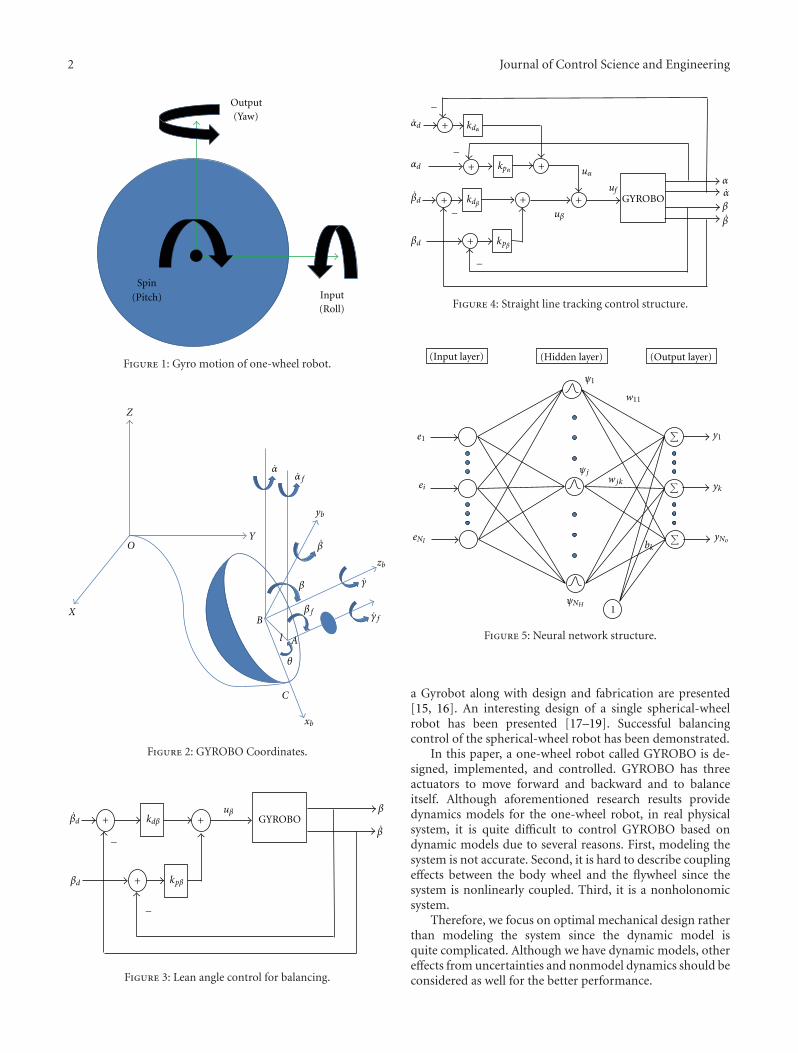
More challengingly, one-wheel mobile robots are devel-oped. A one-wheel robot is a rolling disk that requiresbalancing while running on the ground [6]. Gyrover is atypical disc-typed mobile robot that has been developed andpresented for many years [7–11]. Gyrover is a gyroscopicallystabilized system that uses the gyroscopic motion to balancethe lean angle against falling as shown in Figure 1. Threeactuators are required to make Gyrover stable. Two actuatorsare used for balancing and one actuator for driving. Exper-imental results as well as dynamical modeling analysis onGyrover are well summarized in the literature [12].
In other researches on one-wheel robots, different ap-proaches of modelling dynamics of a one-wheel robot havebeen presented [13, 14]. Simulation studies of controlling
2 Journal of Control Science and Engineering
Spin
(Pitch) Input(Roll)
Output(Yaw)
Figure 1: Gyro motion of one-wheel robot.
γ f
γ
C
l
xb
yb
zb
β f
α fα
β
β
B
θ
YO
X
Z
A
Figure 2: GYROBO Coordinates.
β
β−
−
+
+ +
βd
βd
kpβ
kdβuβ
GYROBO
Figure 3: Lean angle control for balancing.
β
α
GYROBOuf
uβ
uα
+
+
+
+
+
+
+βd
βd
−
−
−
−
αd
αd
kpβ
kdβ
kpα
kdα
α
β
Figure 4: Straight line tracking control structure.
(Input layer) (Hidden layer) (Output layer)
eNI
ψj
ψNH
yk
yNobk
w11
y1e1
eiwjk
ψ1
1
Figure 5: Neural network structure.
a Gyrobot along with design and fabrication are presented[15, 16]. An interesting design of a single spherical-wheelrobot has been presented [17–19]. Successful balancingcontrol of the spherical-wheel robot has been demonstrated.
In this paper, a one-wheel robot called GYROBO is de-signed, implemented, and controlled. GYROBO has threeactuators to move forward and backward and to balanceitself. Although aforementioned research results providedynamics models for the one-wheel robot, in real physicalsystem, it is quite difficult to control GYROBO based ondynamic models due to several reasons. First, modeling thesystem is not accurate. Second, it is hard to describe couplingeffects between the body wheel and the flywheel since thesystem is nonlinearly coupled. Third, it is a nonholonomicsystem.
Therefore, we focus on optimal mechanical design ratherthan modeling the system since the dynamic model isquite complicated. Although we have dynamic models, othereffects from uncertainties and nonmodel dynamics should beconsidered as well for the better performance.

Journal of Control Science and Engineering 3
kix dt
kdx
xd
xd
uβ
ux
eβ(t)
eβ(t − 1)eβ(t − 2)
+
+
+ +
+ +
+
+
−
−
−
−
kpx
GYROBOβ
β
xx
Neuralnetwork
βd
βd
v
kdβ
kpβ
Figure 6: RCT neural network control structure.
Figure 7: Sphere robot with links.
After several modifications of the design, the successfuldesign and control of GYROBO are achieved. Since all ofactuators have to be housed inside the one wheel, design andplacement of each part become the most difficult problem.
After careful design of the system, a neural network con-trol scheme is applied to the model-free-controlled system toimprove balancing performance achieved by linear controll-ers. First, a simple PD control method is applied to the systemand then a neural network controller is added to help the PDcontroller to improve tracking performance. Neural networkhas been known for its capabilities of learning and adaptationfor model-free dynamical systems in online fashion [2, 20].
Experimental studies of a self-balancing task and astraight line tracking task are conducted. Performances by aPD controller and a neural controller are compared.
2. GYROBO Modelling
GYROBO is described as shown in Figure 2. Three anglessuch as spin, lean, and tilt angle are generated by three cor-responding actuators. The gyro effect is created by the com-bination of two angle rotations, flywheel spin and tilt mo-tion.
Table 1: Parameter definition.
α,αf Precession angle of a wheel and a flywheel
β Lean angle of a wheel
β f Tilt angle of a flywheel
γ, γ f Spin angles of a wheel and a flywheel
θ Angle between l and xb axis
mw ,m f Masses of a wheel and a flywheel
m Mass of whole body
R Radius of a wheel
Ixw , Iyw , Izw Wheel moment of inertia about X ,Y , and Z axes
Ix f , Iy f , Iz f Flywheel moment of inertia about X ,Y , and Z
g Gravitational velocity
u1,u2 Drive torque and tilt torque
l Distance between A and B
The dynamics of one-wheel robot system has been pre-sented in [7, 11, 13]. Table 1 lists parameters of GYROBO.This paper is focused on the implementation and control ofGYROBO rather than analyzing the dynamics model of thesystem since the modeling has been well presented in theliterature [11].
Since the GYROBO is a nonholonomic system, there arekinematic constraints such that the robot cannot move in thelateral direction. GYROBO is an underactuated system thathas three actuators to drive more states.
We follow the dynamic equation of the GYROBO des-cribed in [11]:
M(q)q + F
(q, q
) = ATλ + Bu, (1)

4 Journal of Control Science and Engineering
(a) First model (b) Second model
(c) Third model (d) Fourth model
Figure 8: Models of GYROBO using gyro effects.
Figure 9: Real design of GYROBO I.
where
M(q) =
⎡⎢⎢⎢⎢⎢⎢⎢⎢⎢⎢⎢⎣
m 0 0 0 0 0
0 m 0 0 0 0
0 0 M33 0 IzwSβ 0
0 0 0 Ixw + Ix f +mR2S2β 0 Ix f
0 0 IzwSβ 0 Izw 0
0 0 0 Ix f 0 Ix f
⎤⎥⎥⎥⎥⎥⎥⎥⎥⎥⎥⎥⎦,
M33 = IywC2β + IzwS
2β + Iy f C2(β + β f
)+ Iz f S
2(β + β f
),
F(q, q
) =
⎡⎢⎢⎢⎢⎢⎢⎢⎢⎢⎢⎢⎢⎣
0
0
F3
F4
IzwCβαβ
F6
⎤⎥⎥⎥⎥⎥⎥⎥⎥⎥⎥⎥⎥⎦,
(2)
where
F3 = 2(Izw − Iyw
)CβSβαβ + IzwCββγ
+ 2(Iz f − Iy f
)C(β + β f
)S(β + β f
)(β + β f
)α
+ Iz f C(β + β f
)(β + β f
)γ f ,
F4 = mR2SβCββ2 +(Iyw − Izw
)CβSβα2 − IzwCβγα
+(Iy f − Iz f
)C(β + β f
)S(β + β f
)α2
− Iz f C(β + β f
)γ f α−mgRSβ,
F6 =(Iy f − Iz f
)C(β + β f
)S(β + β f
)α2 − Iz f C
(β + β f
)γ f α,
(3)
A =⎡⎣1 0 −RCαCβ RSαSβ −RCα 0
0 1 −RCβCα −RCαCβ −RSα 0
⎤⎦, (4)
Journal of Control Science and Engineering 5
(a)
(b)
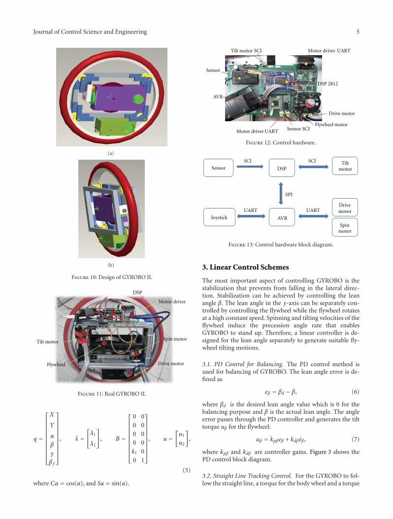
Figure 10: Design of GYROBO II.
Drive motor
Tilt motorSpin motor
DSP
Motor driver
Flywheel
Figure 11: Real GYROBO II.
q =
⎡⎢⎢⎢⎢⎢⎢⎢⎢⎢⎢⎣
X
Y
α
β
γ
β f
⎤⎥⎥⎥⎥⎥⎥⎥⎥⎥⎥⎦, λ =
⎡⎣λ1
λ2
⎤⎦, B =
⎡⎢⎢⎢⎢⎢⎢⎢⎢⎢⎣
0 0
0 0
0 0
0 0
k1 0
0 1
⎤⎥⎥⎥⎥⎥⎥⎥⎥⎥⎦, u =
[u1
u2
],
(5)
where Cα = cos(α), and Sα = sin(α).
Sensor
Tilt motor SCI Motor driver UART
DSP 2812
Flywheel motorSensor SCIMotor driver UART
AVR
Drive motor
Figure 12: Control hardware.
TiltmotorDSP
AVR
Sensor
Joystick
Spinmotor
Drivemotor
SCISCI
UART
SPI
UART
Figure 13: Control hardware block diagram.
3. Linear Control Schemes
The most important aspect of controlling GYROBO is thestabilization that prevents from falling in the lateral direc-tion. Stabilization can be achieved by controlling the leanangle β. The lean angle in the y-axis can be separately con-trolled by controlling the flywheel while the flywheel rotatesat a high constant speed. Spinning and tilting velocities of theflywheel induce the precession angle rate that enablesGYROBO to stand up. Therefore, a linear controller is de-signed for the lean angle separately to generate suitable fly-wheel tilting motions.
3.1. PD Control for Balancing. The PD control method isused for balancing of GYROBO. The lean angle error is de-fined as
eβ = βd − β, (6)
where βd is the desired lean angle value which is 0 for thebalancing purpose and β is the actual lean angle. The angleerror passes through the PD controller and generates the tilttorque uβ for the flywheel:
uβ = kpβeβ + kdβeβ, (7)
where kpβ and kdβ are controller gains. Figure 3 shows thePD control block diagram.
3.2. Straight Line Tracking Control. For the GYROBO to fol-low the straight line, a torque for the body wheel and a torque

6 Journal of Control Science and Engineering
(a) (b)
(c) (d)
(e) (f)
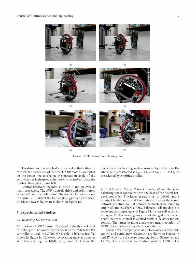
Figure 14: PD control: balancing task (a-b-c-d-e-f in order).
for the flywheel should be separately controlled. The bodywheel rotates to follow the straight line while the lean angleis controlled to maintain balancing.
The position error detected by an encoder is defined by
ep = xd − x, (8)
where xd is the desired position value and x is the actualposition. The detailed PID controller output becomes
ux = kpxex + kdxex + kix
∫exdt, (9)
where kpx, kdx, and kix are controller gains.Thus line tracking control requires both position control
and angle control. The detailed control block diagram for thestraight line following is shown in Figure 4.
4. Neural Control Schemes
4.1. RBF Neural Network Structure. The purpose of using aneural network is to improve the performance controlled bylinear controllers. Linear controllers for controlling
GYROBO may have limited performances since GYROBO isa highly nonlinear and coupled system.
Neural networks have been known for their capabilitiesof learning and adaptation of nonlinear functions and usedfor nonlinear system control [20]. Successful balancingcontrol performances of a two-wheel mobile robot have beenpresented [2].
One of the advantages of using a neural network as anauxiliary controller is that the dynamic model of the system isnot required. The neural network can take care of nonlinearuncertainties in the system by an iterative adaptation processof internal weights.
Here the radial basis function (RBF) network is used foran auxiliary controller to compensate for uncertainties caus-ed by nonlinear dynamics of GYROBO. Figure 5 shows thestructure of the radial basis function.
The Gaussian function used in the hidden layer is
ψj(e) = exp
⎛⎜⎝−∣∣∣e − μ j∣∣∣2
2σ2j
⎞⎟⎠, (10)
where e is the input vector, e = [e1e2 · · · eNI ]T , μ j is

Journal of Control Science and Engineering 7
(a) (b)
(c) (d)
(e) (f)
Figure 15: Neural network control: balancing task.
0 200 400 600 800 1000 1200 1400 1600 1800 2000
0
20
40
60
80
100
120
RCT
PD
−20
Time (ms)
α(d
eg)
Figure 16: Heading angle comparison of PD (black dotted line) andRCT control (blue solid line).
the center value vector of the jth hidden unit, and σ j is thewidth of the jth hidden unit.
The forward kth output in the output layer can be cal-culated as a sum of outputs from the hidden layer:
yk =NH∑j=1
ψjwjk + bk, (11)
where ψj is jth output of the hidden layer in (11), wjk is theweight between the jth hidden unit and kth output, and bk isthe bias weight.
4.2. Neural Network Control. Neural network is utilized togenerate compensating signals to help linear controllers byminimizing the output errors. Initial stability can be achievedby linear controllers and further tracking improvement canbe done by neural network in online fashion.
Different compensation location of neural network yieldsdifferent neural network control schemes, but they eventu-ally perform the same goal to minimize the output error.

8 Journal of Control Science and Engineering
0 200 400 600 800 1000 1200 1400 1600 1800 2000
0
5
10
15
Time (ms)
Desired
RCT
PD
−10
−15
−5
β(d
eg)
Figure 17: Lean angle comparison of PD (black dotted line) andRCT control (blue solid line).
The reference compensation technique (RCT) is known asone of neural network control schemes that provides a struc-tural advantage of not interrupting the predesigned controlstructure [3, 4]. Since the output of neural network is addedto the input trajectories of PD controllers as in Figure 4,tracking performance can be improved. This forms the total-ly separable control structure as an auxiliary controllershown in Figure 6:
uβ = kpβ(eβ + φ1
)+ kdβ
(eβ + φ2
), (12)
where φ1 and φ2 are neural network outputs.Here, the training signal v is selected as a function of
tracking errors such as a form of PD controller outputs:
v = kpβeβ + kdβeβ. (13)
Then (12) becomes
v = uβ −(kpβφ1 + kdβφ2
). (14)
To achieve the inverse dynamic control in (14) such assatisfying the relationship uβ = τ where τ is the dynamics ofGYROBO, we need to drive the training signal of neuralnetwork to satisfy that v → 0. Then the neural network out-puts become equal to the dynamics of the GYROBO in theideal condition. This is known as an inverse dynamics controlscheme. Therefore learning algorithm is developed for theneural network to minimize output errors in the next section.
4.3. Neural Network Learning. Here neural network does notrequire any offline learning process. As an adaptive controll-er, internal weights in neural network are updated at eachsampling time to minimize errors. Therefore, the selection of
an appropriate training signal for the neural networkbecomes an important issue in the neural network control,even it determines the ultimate control performance.The objective function is defined as
E = 12v2. (15)
Differentiating (15) and combining with (14) yield thegradient function required in the back-propagation algo-rithm:
∂E
∂w= v
∂v
∂w= −v
(kpβ
∂φ1
∂w+ kdβ
∂φ2
∂w
). (16)
The weights are updated as
w(t + 1) = w(t) + ηv
(kpβ
∂φ1
∂w+ kdβ
∂φ2
∂w
), (17)
where η is the learning rate.
5. Design of One-Wheel Robot
Design of the one-wheel robot becomes the most importantissue due to the limitation of space. Our first model is shownin Figure 7. The original idea was to balance and control thesphere robot by differing rotating speeds of two links. Thus,two rotational links inside the sphere are supposed to balanceitself but failed due to the irregular momentum induced bytwo links.
After that, the balancing concept has been changed to usea flywheel instead of links to generate gyro effect as shownin Figure 8. Controlling spin and tilt angles of the flywheelyields gyro effects to make the robot keep upright position.
We have designed and built several models as shown inFigure 8. However, all of models are not able to balance itselflong enough. Through trial and error processes of designingmodels, we have a current version of GYROBO I and II asshown in Figures 9 and 10. Since the GYROBO I in Figure 9has a limited space for housing, the second model ofGYROBO has been redesigned as shown in Figure 11.
6. GYROBO Design
Figure 10 shows the CAD design of the GYROBO II. The realdesign consists of motors, a flywheel, and necessary hardwareas shown in Figure 11.
GYROBO II is redesigned with several criteria. Locatingmotors appropriately in the limited space becomes quite animportant problem to satisfy the mass balance. Thus the sizeof the body wheel is increased.
The placement of a flywheel effects the location of thecenter of gravity as well. The size of the flywheel is also criticalin the design to generate enough force to make the wholebody upright position. The size of the flywheel is increased.The frame of the flywheel system is redesigned and located atthe center of the body wheel.
Journal of Control Science and Engineering 9
(a) (b)
(c) (d)
(e) (f)
Figure 18: PD control: line following task.
The drive motor is attached to the wheel so that it directlycontrols the movement of the wheel. A tilt motor is mountedon the center line to change the precession angle of thegyro effect. A high-speed spin motor is located to rotate theflywheel through a timing belt.
Control hardware includes a DSP2812 and an AVR asmain processors. The AVR controls drive and spin motorswhile DSP controls a tilt motor. The detailed layout is shownin Figure 12. To detect the lean angle, a gyro sensor is used.Interface between hardware is shown in Figure 13.
7. Experimental Studies
7.1. Balancing Test at One Point
7.1.1. Scheme 1: PD Control. The speed of the flywheel is setto 7,000 rpm. The control frequency is 10 ms. When the PDcontroller is used, the GYROBO is able to balance itself asshown in Figure 14. However, the heading angle also rotatesas it balances. Figures 14(d), 14(e), and 14(f) show the
deviation of the heading angle controlled by a PD controllerwhose gains are selected as kpβ = 10, and kdβ = 15. PD gainsare selected by empirical studies.
7.1.2. Scheme 2: Neural Network Compensation. The samebalancing test is conducted with the help of the neural net-work controller. The learning rate is set to 0.0005, and 3inputs, 4 hidden units, and 2 outputs are used for the neuralnetwork structure. Neural network parameters are found byempirical studies. The GYROBO balances itself and does notrotate much comparing with Figure 14. It stays still as shownin Figure 15. The heading angle is not changed much whenneural network control is applied while it deviates for PDcontrol. The larger heading angle error means rotation ofGYROBO while balancing which is not desired.
Further clear comparisons of performances between PDcontrol and neural network control are shown in Figures 16and 17, which are the corresponding plots of Figures 14 and15. We clearly see that the heading angle of GYROBO is

10 Journal of Control Science and Engineering
(a) (b)
(c) (d)
(e) (f)
Figure 19: Neural network control: line following.
deviating in the PD control case. We clearly see the largeroscillation of PD control than that of RCT control.
7.2. Line Tracking Test
7.2.1. Scheme 1: PD Control. Next test is to follow the desiredstraight line. Figure 18 shows the line tracking performanceby the PD controller. GYROBO moves forward about 2 mand then stops.
7.2.2. Scheme 2: Neural Network Compensation. Figure 19shows the line tracking performance by the neural networkcontroller.
We see that the GYROBO moves forward while balanc-ing. Since the GYROBO has to carry a power line, navigationis stopped within a short distance about 2 m.
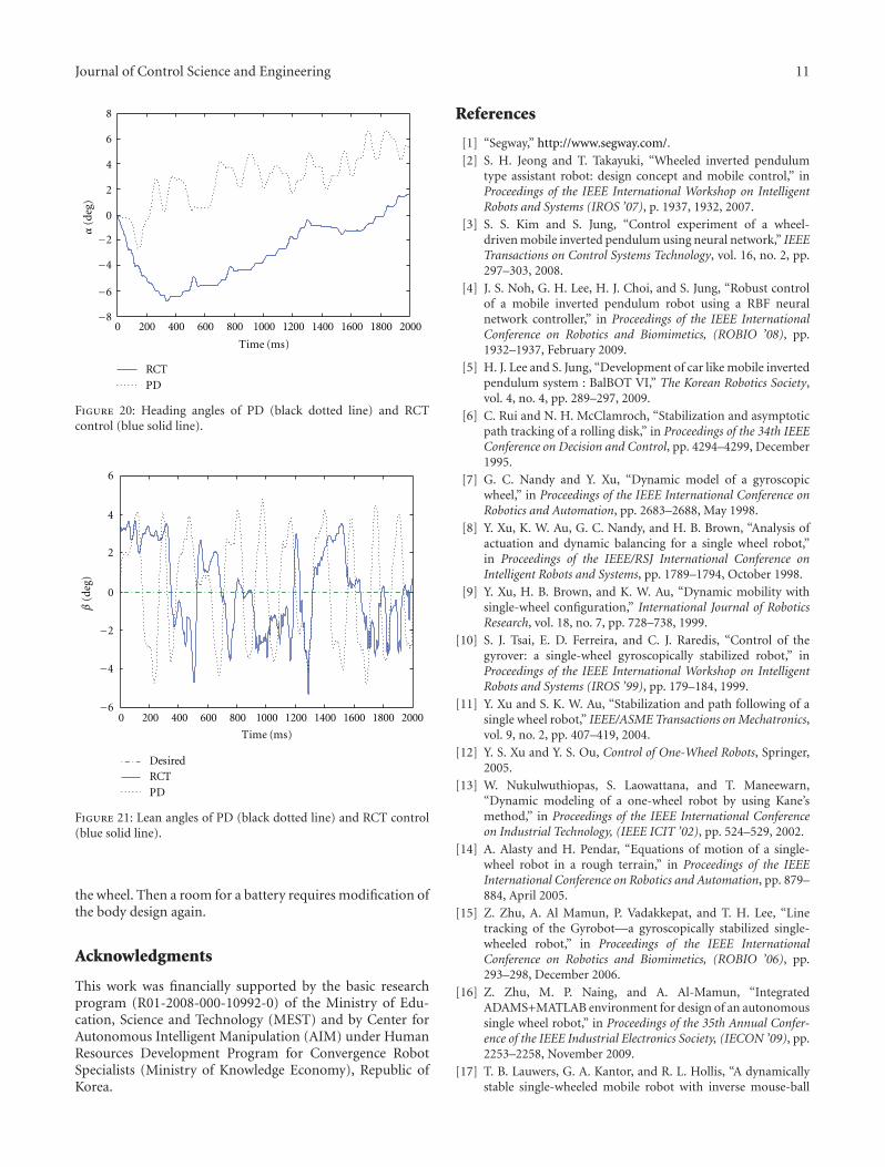
Clear distinctions between PD control and neural net-work control are shown in Figures 20 and 21. Both controll-ers maintain balance successfully. GYROBO controlled by
a PD control method deviates from the desired straight linetrajectory further as described in Figure 20. In addition, theoscillatory behaviour is reduced much by the neural networkcontroller as shown in Figure 21.
8. Conclusion
A one-wheel robot GYROBO is designed and implemented.After several trial errors of body design, successful designis presented. An important key issue is the design topackage all materials in one wheel. One important tip incontrolling GYROBO is to reduce the weight so that theflywheel can generate enough gyro effect because it is noteasy to find suitable motors. Although balancing and linetracking tasks are successful in this paper, one major problemhas to be solved in the future. The power supply for theGYROBO should be independent. Since the stand-alone typeof GYROBO is preferred, a battery should be mounted inside
Journal of Control Science and Engineering 11
0 200 400 600 800 1000 1200 1400 1600 1800 2000
RCT
PD
Time (ms)
0
8
6
4
2
−2
−4
−6
−8
α(d
eg)
Figure 20: Heading angles of PD (black dotted line) and RCTcontrol (blue solid line).
Desired
RCT
PD
0 200 400 600 800 1000 1200 1400 1600 1800 2000
Time (ms)
0
4
2
6
−6
−4
−2
β(d
eg)
Figure 21: Lean angles of PD (black dotted line) and RCT control(blue solid line).
the wheel. Then a room for a battery requires modification ofthe body design again.
Acknowledgments
This work was financially supported by the basic researchprogram (R01-2008-000-10992-0) of the Ministry of Edu-cation, Science and Technology (MEST) and by Center forAutonomous Intelligent Manipulation (AIM) under HumanResources Development Program for Convergence RobotSpecialists (Ministry of Knowledge Economy), Republic ofKorea.
References
[1] “Segway,” http://www.segway.com/.
[2] S. H. Jeong and T. Takayuki, “Wheeled inverted pendulumtype assistant robot: design concept and mobile control,” inProceedings of the IEEE International Workshop on IntelligentRobots and Systems (IROS ’07), p. 1937, 1932, 2007.
[3] S. S. Kim and S. Jung, “Control experiment of a wheel-driven mobile inverted pendulum using neural network,” IEEETransactions on Control Systems Technology, vol. 16, no. 2, pp.297–303, 2008.
[4] J. S. Noh, G. H. Lee, H. J. Choi, and S. Jung, “Robust controlof a mobile inverted pendulum robot using a RBF neuralnetwork controller,” in Proceedings of the IEEE InternationalConference on Robotics and Biomimetics, (ROBIO ’08), pp.1932–1937, February 2009.
[5] H. J. Lee and S. Jung, “Development of car like mobile invertedpendulum system : BalBOT VI,” The Korean Robotics Society,vol. 4, no. 4, pp. 289–297, 2009.
[6] C. Rui and N. H. McClamroch, “Stabilization and asymptoticpath tracking of a rolling disk,” in Proceedings of the 34th IEEEConference on Decision and Control, pp. 4294–4299, December1995.
[7] G. C. Nandy and Y. Xu, “Dynamic model of a gyroscopicwheel,” in Proceedings of the IEEE International Conference onRobotics and Automation, pp. 2683–2688, May 1998.
[8] Y. Xu, K. W. Au, G. C. Nandy, and H. B. Brown, “Analysis ofactuation and dynamic balancing for a single wheel robot,”in Proceedings of the IEEE/RSJ International Conference onIntelligent Robots and Systems, pp. 1789–1794, October 1998.
[9] Y. Xu, H. B. Brown, and K. W. Au, “Dynamic mobility withsingle-wheel configuration,” International Journal of RoboticsResearch, vol. 18, no. 7, pp. 728–738, 1999.
[10] S. J. Tsai, E. D. Ferreira, and C. J. Raredis, “Control of thegyrover: a single-wheel gyroscopically stabilized robot,” inProceedings of the IEEE International Workshop on IntelligentRobots and Systems (IROS ’99), pp. 179–184, 1999.
[11] Y. Xu and S. K. W. Au, “Stabilization and path following of asingle wheel robot,” IEEE/ASME Transactions on Mechatronics,vol. 9, no. 2, pp. 407–419, 2004.
[12] Y. S. Xu and Y. S. Ou, Control of One-Wheel Robots, Springer,2005.
[13] W. Nukulwuthiopas, S. Laowattana, and T. Maneewarn,“Dynamic modeling of a one-wheel robot by using Kane’smethod,” in Proceedings of the IEEE International Conferenceon Industrial Technology, (IEEE ICIT ’02), pp. 524–529, 2002.
[14] A. Alasty and H. Pendar, “Equations of motion of a single-wheel robot in a rough terrain,” in Proceedings of the IEEEInternational Conference on Robotics and Automation, pp. 879–884, April 2005.
[15] Z. Zhu, A. Al Mamun, P. Vadakkepat, and T. H. Lee, “Linetracking of the Gyrobot—a gyroscopically stabilized single-wheeled robot,” in Proceedings of the IEEE InternationalConference on Robotics and Biomimetics, (ROBIO ’06), pp.293–298, December 2006.
[16] Z. Zhu, M. P. Naing, and A. Al-Mamun, “IntegratedADAMS+MATLAB environment for design of an autonomoussingle wheel robot,” in Proceedings of the 35th Annual Confer-ence of the IEEE Industrial Electronics Society, (IECON ’09), pp.2253–2258, November 2009.
[17] T. B. Lauwers, G. A. Kantor, and R. L. Hollis, “A dynamicallystable single-wheeled mobile robot with inverse mouse-ball

12 Journal of Control Science and Engineering
drive,” in Proceedings of the IEEE International Conference onRobotics and Automation, (ICRA ’06), pp. 2884–2889, May2006.
[18] U. Nagarajan, A. Mampetta, G. A. Kantor, and R. L. Hollis,“State transition, balancing, station keeping, and yaw controlfor a dynamically stable single spherical wheel mobile robot,”in Proceedings of the IEEE International Conference on Roboticsand Automation (ICRA’10), pp. 998–1003, 2009.
[19] U. Nagarajan, G. Kantor, and R. L. Hollis, “Trajectory planningand control of an underactuated dynamically stable singlespherical wheeled mobile robot,” in Proceedings of the IEEEInternational Conference on Robotics and Automation, (ICRA’09), pp. 3743–3748, May 2009.
[20] P. K. Kim, J. H. Park, and S. Jung, “Experimental studies ofbalancing control for a disc-typed mobile robot using a neuralcontroller: GYROBO,” in Proceedings of the IEEE InternationalSymposium on Intelligent Control, (ISIC ’10), pp. 1499–1503,September 2010.

Hindawi Publishing CorporationJournal of Control Science and EngineeringVolume 2012, Article ID 867178, 9 pagesdoi:10.1155/2012/867178
Research Article
Robust Adaptive Control via Neural Linearization andCompensation
Roberto Carmona Rodrıguez and Wen Yu
Departamento de Control Automatico, CINVESTAV-IPN, Avenue.IPN 2508, 07360 Mexico City, DF, Mexico
Correspondence should be addressed to Wen Yu, [email protected]
Received 6 October 2011; Revised 4 January 2012; Accepted 5 January 2012
Academic Editor: Isaac Chairez
Copyright © 2012 R. C. Rodrıguez and W. Yu. This is an open access article distributed under the Creative Commons AttributionLicense, which permits unrestricted use, distribution, and reproduction in any medium, provided the original work is properlycited.
We propose a new type of neural adaptive control via dynamic neural networks. For a class of unknown nonlinear systems, aneural identifier-based feedback linearization controller is first used. Dead-zone and projection techniques are applied to assurethe stability of neural identification. Then four types of compensator are addressed. The stability of closed-loop system is alsoproven.
1. Introduction
Feedback control of the nonlinear systems is a big challengefor engineer, especially when we have no complete modelinformation. A reasonable solution is to identify the non-linear, then a adaptive feedback controller can be designedbased on the identifier. Neural network technique seems tobe a very effective tool to identify complex nonlinear systemswhen we have no complete model information or, even,consider controlled plants as “black box”.
Neuroidentifier could be classified as static (feed for-ward) or as dynamic (recurrent) ones [1]. Most of publica-tions in nonlinear system identification use static networks,for example multilayer perceptrons, which are implementedfor the approximation of nonlinear function in the right-side hand of dynamic model equations [2]. The main draw-back of these networks is that the weight updating utilizeinformation on the local data structures (local optima) andthe function approximation is sensitive to the training dates[3]. Dynamic neural networks can successfully overcome thisdisadvantage as well as present adequate behavior in presenceof unmodeled dynamics because their structure incorporatefeedback [4–6].
Neurocontrol seems to be a very useful tool for unknownsystems, because it is model-free control, that is, thiscontroller does not depend on the plant. Many kinds of
neurocontrol were proposed in recent years, for example,supervised neuro control [7] is able to clone the humanactions. The neural network inputs correspond to sensoryinformation perceived by the human, and the outputscorrespond to the human control actions. Direct inversecontrol [1] uses an inverse model of the plant cascaded withthe plant, so the composed system results in an identity mapbetween the desired response and the plant one, but theabsence of feedback dismisses its robustness; internal modelneurocontrol [8] that used forward and inverse model iswithin the feedback loop. Adaptive neurocontrol has twokinds of structure: indirect and direct adaptive control.Direct neuroadaptive may realize the neurocontrol by neuralnetwork directly [1]. The indirect method is the combinationof the neural network identifier and adaptive control, thecontroller is derived from the on-line identification [5].
In this paper we extend our previous results in [9, 10].In [9], the neurocontrol was derived by gradient principal,so the neural control is local optimal. No any restriction isneeded, because the controller did not include the inverseof the weights. In [10], we assume the inverse of theweights exists, so the learning law was normal. The maincontributions of this paper are (1) a special weights updatinglaw is proposed to assure the existence of neurocontrol. (2)Four different robust compensators are proposed. By meansof a Lyapunov-like analysis, we derive stability conditions for

2 Journal of Control Science and Engineering
the neuroidentifier and the adaptive controller. We show thatthe neuroidentifier-based adaptive control is effective for alarge classes of unknown nonlinear systems.
2. Neuroidentifier
The controlled nonlinear plant is given as
xt = f (xt,ut, t), xt ∈ �n, ut ∈ �n, (1)
where f (xt) is unknown vector function. In order to realizeindirect neural control, a parallel neural identifier is used asin [9, 10] (in [5] the series-parallel structure is used):
˙xt = Axt +W1,tσ(xt) +W2,tφ(xt)γ(ut), (2)
where xt ∈ �n is the state of the neural network,W1,t,W2,t ∈�n×n are the weight matrices, A ∈ �n×n is a stable matrix.The vector functions σ(·) ∈ �n, φ(·) ∈ �n×n is a diagonalmatrix. Function γ(·) is selected as ‖γ(ut)‖2 ≤ u., forexample γ(·) may be linear saturation function,
γ(ut) ={ut, if |ut| < b,
u, if |ut| ≥ b.(3)
The elements of the weight matrices are selected as mono-tone increasing functions, a typical presentation is sigmoidfunction:
σi(xt) = ai1 + e−bixt
− ci, (4)
where ai, bi, ci > 0. In order to avoid φ(xt) = 0, we select
φi(xt) = ai1 + e−bixt
+ ci. (5)
Remark 1. The dynamic neural network (2) has beendiscussed by many authors, for example [4, 5, 9, 10]. It can beseen that Hopfield model is the special case of this networkswith A = diag{ai}, ai := −1/RiCi, Ri > 0 and Ci > 0. Ri andCi are the resistance and capacitance at the ith node of thenetwork, respectively.
Let us define identification error as
Δt = xt − xt . (6)
Generally, dynamic neural network (2) cannot follow thenonlinear system (1) exactly. The nonlinear system may bewritten as
xt = Axt +W01σ(xt) +W0
2φ(xt)γ(ut)− ft, (7)
where W01 and W0
2 are initial matrices of W1,t and W2,t
W01Λ
−11 W0T
1 ≤W1, W02Λ
−12 W0T
2 ≤W2. (8)
W1 andW2 are prior known matrices, vector function ft canbe regarded as modelling error and disturbances. Because
σ(·) and φ(·) are chosen as sigmoid functions, clearly theysatisfy the following Lipschitz property:
σTΛ1σ ≤ ΔTt DσΔt,(φtγ(ut)
)TΛ2
(φtγ(ut)
)≤ uΔTt DφΔt,
(9)
where σ = σ(xt)−σ(xt), φ = φ(xt)−φ(xt), Λ1, Λ2, Dσ , andDφ are known positive constants matrices. The error dynamicis obtained from (2) and (7):
Δt = AΔt+W1,tσ(xt)+W2,tφ(xt)γ(ut)+W01 σ+W0
2 φγ(ut)+ ft,(10)
where W1,t =W1,t −W01 , W2,t =W2,t −W0
2 . As in [4, 5, 9,10], we assume modeling error is bounded.
(A1) the unmodeled dynamic f satisfies
f Tt Λ−1f ft ≤ η. (11)
Λ f is a known positive constants matrix.If we define
R =W1 +W2 + Λ f , Q = Dσ + uDφ +Q0, (12)
and the matrices A and Q0 are selected to fulfill the followingconditions:
(1) the pair (A,R1/2) is controllable, the pair (Q1/2,A) isobservable,
(2) local frequency condition [9] satisfies frequencycondition:
ATR−1A−Q ≥ 14
[ATR−1 − R−1A
]R[ATR−1 − R−1A
]T,
(13)
then the following assumption can be established.
(A2) There exist a stable matrix A and a strictly positivedefinite matrix Q0 such that the matrix Riccatiequation:
ATP + PA + PRP +Q = 0 (14)
has a positive solution P = PT > 0.This condition is easily fulfilled if we select A as stable
diagonal matrix. Next Theorem states the learning procedureof neuroidentifier.
Theorem 2. Subject to assumptions A1 and A2 being satis-fied, if the weights W1,t and W2,t are updated as
W1,t = st[−K1PΔtσ
T(xt)]
,
W2,t = stPr[−K2Pφ(xt)γ(ut)ΔTt
],
(15)

Journal of Control Science and Engineering 3
where K1, K2 > 0, P is the solution of Riccati equation (14),Pri[ω] (i = 1, 2) are projection functions which are defined asω = K2Pφ(xt)γ(ut)ΔTt
Pr[−ω] =
⎧⎪⎪⎪⎨⎪⎪⎪⎩−ω, condition,
−ω +
∥∥∥W2,t
∥∥∥2
tr(WT
2,t(K2P)W2,t
)ω otherwise,(16)
where the “condition” is ‖W2,t‖ < r or [‖W2,t‖ =r and tr(−ωW2,t) ≤ 0], r < ‖W0
2‖ is a positive constant. stis a dead-zone function
st ={
1, if ‖Δt‖2 > λ−1min(Q0)η,
0, otherwise,(17)
then the weight matrices and identification error remainbounded, that is,
Δt ∈ L∞, W1,t ∈ L∞, W2,t ∈ L∞, (18)
for any T > 0 the identification error fulfills the followingtracking performance:
1T
∫ T0‖Δt‖2
Q0dt ≤ κη +
ΔT0 PΔ0
T, (19)
where κ is the condition number of Q0 defined as κ =λmax(Q0)/λmin(Q0).
Proof. Select a Lyapunov function as
Vt = ΔTt PΔt + tr{WT
1,tK−11 W1,t
}+ tr
{WT
2,tK−12 W2,t
}, (20)
where P ∈ �n×n is positive definite matrix. According to(10), the derivative is
Vt = ΔTt(PA + ATP
)Δt + 2ΔTt PW1,tσ(xt)
+ 2ΔTt PW2,tφ(xt)γ(ut) + 2ΔTt P ft
+ 2ΔTt P[W∗
1 σ +W∗1 φγ(ut)
]+ 2 tr
{˙WT
1,tK−11 W1,t
}+ 2 tr
{˙WT
2,tK−12 W2,t
}.
(21)
Since ΔTt PW∗1 σt is scalar, using (9) and matrix inequality
XTY +(XTY
)T ≤ XTΛ−1X + YTΛY , (22)
where X ,Y ,Λ ∈ �n×k are any matrices, Λ is any positivedefinite matrix, we obtain
2ΔTt PW∗1 σt ≤ ΔTt PW
∗1 Λ
−11 W∗T
1 PΔt + σTt Λ1σt
≤ ΔTt(PW1P +Dσ
)Δt,
2ΔTt PW∗2 φtγ(ut) ≤ ΔTt
(PW2P + uDφ
)Δt .
(23)
In view of the matrix inequality (22) and (A1),
2ΔTt P ft ≤ ΔTt PΛ f PΔt + η. (24)
So we have
Vt ≤ ΔTt[PA + ATP + P
(W1 +W2 + Λ f
)P
+(Dσ + uDφ +Q0
)]Δt
+ 2 tr{
˙WT
1,tK−11 W1,t
}+ 2ΔTt PW1,tσ(xt) + η − ΔTt Q0Δt
+ 2 tr{
˙WT
2,tK−12 W2,t
}+ 2ΔTt PW2,tφ(xt)γ(ut).
(25)
Since ˙W1,t = W1,t and ˙W2,t = W2,t, if we use (A2), we have
Vt ≤ 2 tr{[K−1
1 WT1,t + K1PΔtσ
T(xt)]W1,t
}+ η − ΔTt Q0Δt
+ 2 tr{[K−1
2 W2,t + Pφ(xt)γ(ut)ΔTt]W2,t
}.
(26)
(I) if ‖Δt‖2 > λ−1min(Q0)η, using the updating law as (15)
we can conclude that
Vt ≤ 2 tr{[
Pr[Pφ(xt)γ(ut)ΔTt
]+ Pφ(xt)γ(ut)ΔTt
]W2,t
}− ΔTt Q0Δt + η,
(27)
(a) if ‖W2,t‖ < r or [‖W2,t‖ = r and tr(−ωW2,t) ≤0], Vt ≤ −λmin(Q0)‖Δt‖2 + η < 0,
(b) if ‖W2,t‖ = r and tr(−ωW2,t) > 0
Vt ≤ 2 tr
⎧⎪⎨⎪⎩K2P
∥∥∥W2,t
∥∥∥2
tr(WT
2,t(K2P)W2,t
)ωW2,t
⎫⎪⎬⎪⎭− ΔTt Q0Δt + η
≤ −ΔTt Q0Δt + η < 0.(28)
Vt is bounded. Integrating (27) from 0 up to Tyields
VT −V0 ≤ −∫ T
0ΔTt Q0Δtdt + ηT. (29)
Because κ ≥ 1, we have∫ T0ΔTt Q0Δtdt ≤ V0 −VT +
∫ T0ΔTt Q0Δtdt ≤ V0 + ηT ,
≤ V0 + κηT ,(30)
where κ is condition number of Q0
(II) If ‖Δt‖2 ≤ λ−1min(Q0)η, the weights become constants,
Vt remains bounded. And
∫ T0ΔTt Q0Δtdt ≤
∫ T0λmax(Q0)‖Δt‖2dt
≤ λmax(Q0)λmin(Q0)
ηT ≤ V0 + κηT.
(31)
From (I) and (II), Vt is bounded, (18) is realized. From(20) and W1,t =W1,t −W0
1 ,W2,t =W2,t −W02 we know V0 =
ΔT0 PΔ0. Using (30) and (31), (19) is obtained. The theoremis proved.

4 Journal of Control Science and Engineering
−W2,tW2,t
W∗2
W02
W02
W2,t
r
W2,t
Figure 1: Projection algorithm.
Remark 3. The weight update law (15) uses two techniques.The dead-zone st is applied to overcome the robust problem
caused by unmodeled dynamic ft. In presence of distur-bance or unmodeled dynamics, adaptive procedures mayeasily go unstable. The lack of robustness of parametersidentification was demonstrated in [11] and became a hotissue in 1980s. Dead-zone method is one of simple andeffective tool. The second technique is projection approachwhich may guarantee that the parameters remain withina constrained region and do not alter the properties ofthe adaptive law established without projection [12]. Theprojection approach proposed in this paper is explainedin Figure 1. We hope to force W2,t inside the ball ofcenter W0
2 and radius r. If ‖W2,t‖ < r, we use thenormal gradient algorithm. When W2,t −W0
2 is on the ball,and the vector W2,t points either inside or along the ball,
that is, (d/dt)‖W2,t‖2 = 2 tr(−ωW2,t) ≤ 0, we also keep this
algorithm. If tr(−ωW2,t) > 0, tr[(−ω + (‖W2,t‖2/ tr(WT
2,t
(K2P)W2,t))ω)W2,t] < 0, so (d/dt)‖W2,t‖2< 0,W2,t are di-
rected toward the inside or the ball, that is, W2,t will neverleave the ball. Since r < ‖W0
2‖,W2,t /= 0.
Remark 4. Figure 1 and (7) show that the initial conditionsof the weights influence identification accuracy. In order tofind good initial weights, we design an offline method. Fromabove theorem, we know the weights will convergence to azone. We use any initial weights, W0
1 and W02, after T0, the
identification error should become smaller, that is,W1,T0 andW2,T0 are better than W0
1 and W02 . We use following steps to
find the initial weights.
(1) Start from any initial value for W01 = W1,0, W0
2 =W2,0.
(2) Do identification until training time arrives T0.
(3) If the ‖Δ(T0)‖ < ‖Δ(0)‖, letW1,T0 ,W2,T0 as a newW01
and W02 , go to 2 to repeat the identification process.
(4) If the ‖Δ(T0)‖ ≥ ‖Δ(0)‖, stop this offline identifica-tion, now W1,T0 , W2,T0 are the final initial weights.
Remark 5. Since the updating rate is KiP (i = 1, 2), and Kican be selected as any positive matrix, the learning processof the dynamic neural network (15) is free of the solution ofRiccati equation (14).
Remark 6. Let us notice that the upper bound (19) turnsout to be “sharp”, that is, in the case of not having any
uncertainties (exactly matching case: f = 0) we obtain η = 0and, hence,
lim supT→∞
1T
∫ T0‖Δt‖2
Q0dt = 0 (32)
from which, for this special situation, the asymptotic stabilityproperty (‖Δt‖ →
t→∞ 0) follows. In general, only the
asymptotic stability “in average” is guaranteed, because thedead-zone parameter η can be never set zero.
3. Robust Adaptive Controller Based onNeuro Identifier
From (7) we know that the nonlinear system (1) may bemodeled as
xt = Axt +W∗1 σ(xt) +W∗
2 φ(xt)γ(ut) + f
= Axt +W1,tσ(xt) +W2,tφ(xt)γ(ut)
+ f +W1,tσ(xt)+W2,tφ(xt)γ(ut)+W∗1,t σt+W
∗1 φγ(ut).
(33)
Equation (33) can be rewritten as
xt = Axt +W1,tσ(xt) +W2,tφ(xt)γ(ut) + dt , (34)
where
dt = f + W1,tσ(xt) + W2,tφ(xt)γ(ut) +W∗1,tσt +W∗
1 φγ(ut).(35)
If updated law of W1,t and W2,t is (15), W1,t and W2,t arebounded. Using the assumption (A1), dt is bounded as d =supt‖dt‖.
The object of adaptive control is to force the nonlinearsystem (1) following a optimal trajectory x∗t ∈ �r which isassumed to be smooth enough. This trajectory is regarded asa solution of a nonlinear reference model:
x∗t = ϕ(x∗t , t
), (36)
with a fixed initial condition. If the trajectory has pointsof discontinuity in some fixed moments, we can use anyapproximating trajectory which is smooth. In the case ofregulation problem ϕ(x∗t , t) = 0, x∗(0) = c, c is constant.Let us define the sate trajectory error as
Δ∗t = xt − x∗t . (37)

Journal of Control Science and Engineering 5
From (34) and (36) we have
Δ∗t = Axt +W1,tσ(xt) +W2,tφ(xt)γ(ut) + dt − ϕ(x∗t , t
).
(38)
Let us select the control action γ(ut) as linear form
γ(ut) = U1,t +[W2,tφ(xt)
]−1U2,t, (39)
where U1,t ∈ �n is direct control part and U2,t ∈ �n is acompensation of unmodeled dynamic dt . As ϕ(x∗t , t), x∗t ,W1,tσ(xt) and W2,tφ(xt) are available, we can select U1,t as
U1,t =[W2,tφ(xt)
]−1[ϕ(x∗t , t
)− Ax∗t −W1,tσ(xt)]. (40)
Because φ(xt) in (5) is different from zero, and W2,t /= 0 bythe projection approach in Theorem 2. Substitute (39) and(40) into (38), we have So the error equation is
Δ∗t = AΔ∗t +U2,t + dt . (41)
Four robust algorithms may be applied to compensate dt .
(A) Exactly Compensation. From (7) and (2) we have
dt =(xt − ˙xt
)− A(xt − xt). (42)
If xt is available, we can select U2,t as Ua2,t = −dt , that is,
Ua2,t = A(xt − xt)−
(xt − ˙xt
). (43)
So, the ODE which describes the state trajectory error is
Δ∗t = AΔ∗t . (44)
Because A is stable, Δ∗t is globally asymptotically stable.
limt→∞Δ
∗t = 0. (45)
(B) An Approximate Method. If xt is not available, anapproximate method may be used as
xt = xt − xt−ττ
+ δt, (46)
where δt > 0, is the differential approximation error. Let usselect the compensator as
Ub2,t = A(xt − xt)−
(xt − xt−τ
τ− ˙xt
). (47)
So Ub2,t = Ua
2,t + δt, (44) become
Δ∗t = AΔ∗t + δt . (48)
Define Lyapunov-like function as
Vt = Δ∗Tt P2Δ∗t , P2 = PT2 > 0. (49)
The time derivative of (49) is
Vt = Δ∗t(ATP2 + P2A
)Δ∗t + 2Δ∗Tt P2δt, (50)
2ΔTt P2δt can be estimated as
2Δ∗Tt P2δt ≤ Δ∗Tt P2ΛP2Δ∗t + δTt Λ
−1δt (51)
where Λ is any positive define matrix. So (50) becomes
Vt≤Δ∗t(ATP2 +P2A+P2ΛP2 +Q2
)Δ∗t +δTt Λ
−1δt−Δ∗Tt Q2Δ∗t ,
(52)
where Q is any positive define matrix. Because A is stable,there exit Λ and Q2 such that the matrix Riccati equation:
ATP2 + P2A + P2ΛP2 +Q2 = 0 (53)
has positive solution P2 = PT2 > 0. Defining the followingseminorms: ∥∥Δ∗t ∥∥2
Q2= lim
T→∞1T
∫ T0Δ∗t Q2Δ
∗t dt, (54)
where Q2 = Q2 > 0 is the given weighting matrix, thestate trajectory tracking can be formulated as the followingoptimization problem:
Jmin = minut
J , J = ∥∥xt − x∗t ∥∥2Q2. (55)
Note that
limT→∞
1T
(Δ∗T0 P2Δ
∗0
)= 0 (56)
based on the dynamic neural network (2), the control law(47) can make the trajectory tracking error satisfies thefollowing property: ∥∥Δ∗t ∥∥2
Q2≤ ‖δt‖2
Λ−1 . (57)
A suitable selection of Λ and Q2 can make the Riccatiequation (53) has positive solution and make ‖Δ∗t ‖2
Q2small
enough if τ is small enough.
(C) Sliding Mode Compensation. If xt is not available,the sliding mode technique may be applied. Let us defineLyapunov-like function as
Vt = Δ∗Tt P3Δ∗t , (58)
where P3 is a solution of the Lyapunov equation:
ATP3 + P3A = −I. (59)
Using (41) whose time derivative is
Vt = Δ∗t(ATP3 + P3A
)Δ∗t + 2Δ∗Tt P3U2,t + 2Δ∗Tt P3dt . (60)
According to sliding mode technique, we may select u2,t as
Uc2,t = −kP−1
3 sgn(Δ∗t), k > 0, (61)
where k is positive constant,
sgn(Δ∗t) =
⎧⎪⎪⎨⎪⎪⎩1 Δ∗t > 0
0 Δ∗t = 0
−1 Δ∗t < 0
sgn(Δ∗t) = [sgn
(Δ∗1,t
), . . . sgn
(Δ∗n,t
)]T ∈ �n.
(62)
6 Journal of Control Science and Engineering
Substitute (59) and (61) into (60)
Vt = −∥∥Δ∗t ∥∥2 − 2k
∥∥Δ∗t ∥∥ + 2Δ∗Tt Pdt
≤ −∥∥Δ∗t ∥∥2 − 2k∥∥Δ∗t ∥∥ + 2λmax(P)
∥∥Δ∗t ∥∥‖dt‖= −∥∥Δ∗t ∥∥2 − 2
∥∥Δ∗t ∥∥(k − λmax(P)‖dt‖).
(63)
If we select
k > λmax(P3)d, (64)
where d is define as (35), then Vt < 0. So,
limt→∞Δ
∗t = 0. (65)
(D) Local Optimal Control. If xt is not available and xt is notapproximated as (B). In order to analyze the tracking errorstability, we introduce the following Lyapunov function:
Vt(Δ∗t) = Δ∗t P4Δ
∗t , P4 = PT4 > 0. (66)
Using (41), whose time derivative is
V t = Δ∗t(ATP4 + P4A
)Δ∗t + 2Δ∗Tt P4U2,t + 2Δ∗Tt P4dt , (67)
2Δ∗Tt P4dt can be estimated as
2Δ∗Tt P4dt ≤ Δ∗t P4Λ−14 P4Δ
∗t + dTt Λ4dt . (68)
Substituting (68) in (67), adding and subtracting the termΔ∗Tt Q4Δ
∗t and UdT
2,t R4Ud2,t with Q4 = QT
4 > 0 and R4 = RT4 >0, we formulate
V t ≤ Δ∗t(ATP4 + P4A + P4Λ4P4 +Q4
)Δ∗t
+ 2Δ∗Tt P4Ud2,t +UdT
2,t R4Ud2,t + dTt Λ
−14 dt − Δ∗t QΔ
∗t
−UdT2,t R4U
d2,t .
(69)
Because A is stable, there exit Λ4 and Q4 such that the matrixRiccati equation:
ATP4 + P4A + P4Λ4P4 +Q4 = 0. (70)
So (69) is
V t ≤ −(∥∥Δ∗t ∥∥2
Q4+∥∥∥Ud
2,t
∥∥∥2
R4
)+ Ψ
(Ud
2,t
)+ dTt Λ
−14 dt, (71)
where
Ψ(Ud
2,t
)= 2Δ∗Tt P4U
d2,t +UdT
2,t R4Ud2,t . (72)
We reformulate (71) as∥∥Δ∗t ∥∥2Q4
+∥∥∥Ud
2,t
∥∥∥2
R4≤ Ψ
(Ud
2,t
)+ dTt Λ
−14 dt −V t . (73)
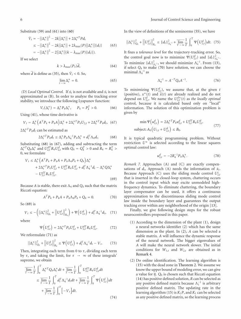
Then, integrating each term from 0 to τ, dividing each termby τ, and taking the limit, for τ → ∞ of these integrals’supreme, we obtain
limT→∞
1T
∫ T0Δ∗Tt Q4Δ
∗t dt + lim
T→∞1T
∫ T0UdT
2,t R4Ud2,tdt
≤ limT→∞
1T
∫ T0dTt Λ
−14 dtdt + lim
T→∞1T
∫ T0Ψ(Ud
2,t
)dt
+ limT→∞
1T
∫ T0
[−V t
]dt.
(74)
In the view of definitions of the seminorms (55), we have
∥∥Δ∗t ∥∥2Q4
+∥∥∥Ud
2,t
∥∥∥2
R4≤ ‖dt‖2
Λ−14
+ limT→∞
1T
∫ T0Ψ(Ud
2,t
)dt. (75)
It fixes a tolerance level for the trajectory-tracking error. So,the control goal now is to minimize Ψ(Ud
2,t) and ‖dt‖2Λ−1
4.
To minimize ‖dt‖2Λ−1
4, we should minimize Λ−1
4 . From (13),if select Q4 to make (70) have solution, we can choose theminimal Λ−1
4 as
Λ−14 = A−TQ4A
−1. (76)
To minimizing Ψ(Ud2,t), we assume that, at the given t
(positive), x∗(t) and x(t) are already realized and do notdepend on Ud
2,t. We name the Ud∗2,t (t) as the locally optimal
control, because it is calculated based only on “local”information. The solution of this optimization problem isgiven by
minΨ(ud2,t
)= 2Δ∗Tt P4u
d2,t +UdT
2,t R4Ud2,t .
subject:A0
(U1,t +Ud
2,t
)≤ B0.
(77)
It is typical quadratic programming problem. Withoutrestriction U∗ is selected according to the linear squaresoptimal control law:
ud2,t = −2R−14 P4Δ
∗t . (78)
Remark 7. Approaches (A) and (C) are exactly compen-sations of dt, Approach (A) needs the information of xt.Because Approach (C) uses the sliding mode control Uc
2,t
that is inserted in the closed-loop system, chattering occursin the control input which may excite unmodeled high-frequency dynamics. To eliminate chattering, the boundarylayer compensator can be used, it offers a continuousapproximation to the discontinuous sliding mode controllaw inside the boundary layer and guarantees the outputtracking error within any neighborhood of the origin [13].
Finally, we give following design steps for the robustneurocontrollers proposed in this paper.
(1) According to the dimension of the plant (1), designa neural networks identifier (2) which has the samedimension as the plant. In (2), A can be selected astable matrix. A will influence the dynamic responseof the neural network. The bigger eigenvalues ofA will make the neural network slower. The initialconditions for W1,t and W2,t are obtained as inRemark 4.
(2) Do online identification. The learning algorithm is(15) with the dead zone in Theorem 2. We assume weknow the upper bound of modeling error, we can givea value for η. Q0 is chosen such that Riccati equation(14) has positive defined solution,R can be selected asany positive defined matrix because Λ−1
1 is arbitrarypositive defined matrix. The updating rate in thelearning algorithm (15) isK1P, andK1 can be selectedas any positive defined matrix, so the learning process

Journal of Control Science and Engineering 7
is free of the solution P of the Riccati equations (14).The larger K1P is selected, the faster convergence theneuroidentifier has.
(3) Use robust control (39) and one of compensation of(43), (47), (61), and (78).
4. Simulation
In this section, a two-link robot manipulator is used toillustrate the proposed approach. Its dynamics of can beexpressed as follows [14]:
M(θ)..
θ +V(θ, θ
)θ +G(θ) + Fd
(θ)= τ, (79)
where θ ∈ �2 consists of the joint variables, θ ∈ �2
denotes the links velocity, τ is the generalized forces, M(θ)is the intertie matrix, V(θ, θ) is centripetal-Coriolis matrix,and G(θ) is gravity vector, Fd(θ) is the friction vector. M(θ)represents the positive defined inertia matrix. If we definex1 = θ = [θ1, θ2] is joint position, x2 = θ is joint velocityof the link, xt = [x1, x2]T , (79) can be rewritten as state spaceform [15]:
x1 = x2,
x2 = H(xt,ut),(80)
where ut = τ is control input,
H(xt,ut) = −M(x1)−1[C(x1, x2)x1 +G(x1) + Fx1 + ut].(81)
Equation (80) can also be rewritten as
x1 =∫ t
0H(xτ ,uτ)dτ +H(x0,u0). (82)
So the dynamic of the two-link robot (79) is in form of (1)with
f (xt,ut, t) =∫ t
0H(xτ ,uτ)dτ +H(x0,u0). (83)
The values of the parameters are listed below: m1 = m2 =1.53 kg, l1 = l2 = 0.365 m, r1 = r2 = 0.1, v1 = v2 =0.4, k1 = k2 = 0.8. Let define x = [θ1, θ2]
T, and u =
[τ1, τ2]T , the neural network for control is represented as
˙x = Ax +W1,tσ(xt) +W2,tφ(x)u. (84)
We select A = [−1.5 00 −1
], φ(xt) = diag(φ1(x1),φ2(x2)),
σ(xt) = [σ2(x2), σ2(x2)]T
σi(xi) = 2(1 + e−2xi
) − 12
,
φi(xi) = 2(1 + e−2xi
) +12
,(85)
where i = 1, 2. We used Remark 4 to obtain a suitable W01
and W02 , start from random values, T0 = 100. After 2 loops,
‖Δ(T0)‖ does not decrease, we let theW1,300 andW2,300 as the
0 500 1000 1500 2000 2500 3000
0
2
4
6
PD control
Neurocontrol
−6
−4
−2
Figure 2: Tracking control of θ1 (method B).
new W01 =
[0.51 3.8−2.3 1.51
]and W0
2 =[
3.12 −2.785.52 −4.021
]. For the update
laws (15), we select η = 0.1, r = 5, K1P = K1P =[
5 00 2
]. If we
select the generalized forces as
τ1 = 7 sin t, τ2 = 0. (86)
Now we check the neurocontrol. We assume the robotis changed at t = 480, after that m1 = m2 = 3.5 kg, l1 =l2 = 0.5 m, and the friction becomes disturbance asD sin((π/3)t), D is a positive constant. We compare neuro-control with a PD control as
τPD = −10(θ − θ∗)− 5(θ − θ∗
), (87)
where θ∗1 = 3; θ∗2 is square wave. So ϕ(θ∗) = θ∗ = 0.The neurocontrol is (39)
τneuro =[W2,tφ(x)
]+[ϕ(x∗t , t
)− Ax∗t −W1,tσ(x)]
+[W2,tφ(x)
]+U2,t .
(88)
U2,t is selected to compensate the unmodeled dynamics. Sinef is unknown method. (A) exactly compensation, cannot beused.
(B) D = 1. The link velocity θ is measurable, as in (43),
U2,t = A(θ − θ
)−(θ − ˙
θ). (89)
The results are shown in Figures 2 and 3.(C) D = 0.3. θ is not available, the sliding mode
technique may be applied. we select u2,t as (61).
u2,t = −10× sgn(θ − θ∗). (90)
The results are shown in Figures 4 and 5.(D) D = 3. We select Q = 1/2, R = 1/20, Λ = 4.5, the
solution of following Riccati equation:
ATP + PA + PΛPt +Q = −P (91)
is P = [0.33 0
0 0.33
]. If without restriction τ, the linear squares
optimal control law:
u2,t = −2R−1P(θ − θ∗) =[−20 0
0 −20
](θ − θ∗). (92)

8 Journal of Control Science and Engineering
0 500 1000 1500 2000 2500 3000
0
2
4
Neurocontrol
PD control
−10
−8
−6
−2
−4
Figure 3: Tracking control of θ2 (method B).
0 500 1000 1500 2000 2500
0
2
4
6
Neurocontrol
PD control
−6
−4
−2
Figure 4: Tracking control of θ1 (method C).
0 500 1000 1500 2000 2500
0
2
4
6
8
NeurocontrolPD control
−10
−8
−6
−4
−2
Figure 5: Tracking control of θ2 (method C).
0 100 200 300 400 500 600 700 800
0
2
4
6
8PD control
Neurocontrol
−6
−4
−2
Figure 6: Tracking control of θ1 (method D).
−10
−8
−6
−4
−2
0 100 200 300 400 500 600 700 800
0
2
4
6
Neurocontrol
PD control
Figure 7: Tracking control of θ2 (method D).
The results of local optimal compensation are shown inFigures 6 and 7.
We may find that the neurocontrol is robust and effectivewhen the robot is changed.
5. Conclusion
By means of Lyapunov analysis, we establish bounds for boththe identifier and adaptive controller. The main contribu-tions of our paper is that we give four different compensationmethods and prove the stability of the neural controllers.
References
[1] K. S. Narendra and K. Parthasarathy, “Identi cation andcontrol for dynamic systems using neural networks,” IEEETransactions on Neural Networks, vol. 1, pp. 4–27, 1990.
[2] S. Jagannathan and F. L. Lewis, “Identi cation of nonlineardynamical systems using multilayered neural networks,” Auto-matica, vol. 32, no. 12, pp. 1707–1712, 1996.
[3] S. Haykin, Neural Networks-A comprehensive Foundation,Macmillan College, New York, NY, USA, 1994.

Journal of Control Science and Engineering 9
[4] E. B. Kosmatopoulos, M. M. Polycarpou, M. A. Christodou-lou, and P. A. Ioannou, “High-order neural network structuresfor identification of dynamical systems,” IEEE Transactions onNeural Networks, vol. 6, no. 2, pp. 422–431, 1995.
[5] G. A. Rovithakis and M. A. Christodoulou, “Adaptive controlof unknown plants using dynamical neural networks,” IEEETransactions on Systems, Man and Cybernetics, vol. 24, no. 3,pp. 400–412, 1994.
[6] W. Yu and X. Li, “Some new results on system identi cationwith dynamic neural networks,” IEEE Transactions on NeuralNetworks, vol. 12, no. 2, pp. 412–417, 2001.
[7] E. Grant and B. Zhang, “A neural net approach to supervisedlearning of pole placement,” in Proceedings of the IEEESymposium on Intelligent Control, 1989.
[8] K. J. Hunt and D. Sbarbaro, “Neural networks for nonlinearinternal model control,” IEE Proceedings D—Control Theoryand Applications, vol. 138, no. 5, pp. 431–438, 1991.
[9] A. S. Poznyak, W. Yu, E. N. Sanchez, and J. P. Perez, “Nonlinearadaptive trajectory tracking using dynamic neural networks,”IEEE Transactions on Neural Networks, vol. 10, no. 6, pp. 1402–1411, 1999.
[10] W. Yu and A. S. Poznyak, “Indirect adaptive control via paralleldynamic neural networks,” IEE Proceedings Control Theory andApplications, vol. 146, no. 1, pp. 25–30, 1999.
[11] B. Egardt, Stability of Adaptive Controllers, vol. 20 of LectureNotes in Control and Information Sciences, Springer, Berlin,Germany, 1979.
[12] P. A. Ioannou and J. Sun, Robust Adaptive Control, Prentice-Hall, Upper Saddle River, NJ, USA, 1996.
[13] M. J. Corless and G. Leitmann, “Countinuous state feed-back guaranteeing uniform ultimate boundness for uncertaindynamic systems,” IEEE Transactions on Automatic Control,vol. 26, pp. 1139–1144, 1981.
[14] F. L. Lewis, A. Yesildirek, and K. Liu, “Multilayer neural-netrobot controller with guaranteed tracking performance,” IEEETransactions on Neural Networks, vol. 7, no. 2, pp. 388–399,1996.
[15] S. Nicosia and A. Tornambe, “High-gain observers in thestate and parameter estimation of robots having elastic joins,”System & Control Letter, vol. 13, pp. 331–337, 1989.

Hindawi Publishing CorporationJournal of Control Science and EngineeringVolume 2012, Article ID 761019, 11 pagesdoi:10.1155/2012/761019
Research Article
Dynamics Model Abstraction Scheme UsingRadial Basis Functions
Silvia Tolu,1 Mauricio Vanegas,2 Rodrigo Agıs,1 Richard Carrillo,1 and Antonio Canas1
1 Department of Computer Architecture and Technology, CITIC ETSI Informatica y de Telecomunicacion, University of Granada, Spain2 PSPC Group, Department of Biophysical and Electronic Engineering (DIBE), University of Genoa, Italy
Correspondence should be addressed to Silvia Tolu, [email protected]
Received 27 July 2011; Accepted 24 January 2012
Academic Editor: Wen Yu
Copyright © 2012 Silvia Tolu et al. This is an open access article distributed under the Creative Commons Attribution License,which permits unrestricted use, distribution, and reproduction in any medium, provided the original work is properly cited.
This paper presents a control model for object manipulation. Properties of objects and environmental conditions influence themotor control and learning. System dynamics depend on an unobserved external context, for example, work load of a robotmanipulator. The dynamics of a robot arm change as it manipulates objects with different physical properties, for example, themass, shape, or mass distribution. We address active sensing strategies to acquire object dynamical models with a radial basisfunction neural network (RBF). Experiments are done using a real robot’s arm, and trajectory data are gathered during varioustrials manipulating different objects. Biped robots do not have high force joint servos and the control system hardly compensatesall the inertia variation of the adjacent joints and disturbance torque on dynamic gait control. In order to achieve smoother controland lead to more reliable sensorimotor complexes, we evaluate and compare a sparse velocity-driven versus a dense position-drivencontrol scheme.
1. Introduction
Current research of biomorphic robots can highly benefitfrom simulations of advance learning paradigms [1–5] andalso from knowledge acquired from biological systems [6–8].The basic control of robot actuators is usually implementedby adopting a classic scheme [9–14]: (a) the desired trajec-tory, in joint coordinates, is obtained using the inverse kine-matics [12, 14, 15] and (b) efficient motor commands drive,for example, an arm, making use of the inverse dynamicsmodel or using high power motors to achieve rigid move-ments. Different controlling schemes using hybrid posi-tion/velocity and forces have been introduced mainly forindustrial robots [9, 10]. In fact, industrial robots areequipped with digital controllers, generally of PID type withno possibility of modifying the control algorithms to im-prove their performance. Robust control (control using PIDparadigms [12, 14–19]) is very power consuming and highlyreduces autonomy of nonrigid robots. Traditionally, themajor application of industrial robots is related to tasks thatrequire only position control of the arm. Nevertheless, thereare other important robotic tasks that require interaction
between the robot’s end-effector and the environment. Sys-tem dynamics depend on an unobserved external context[3, 20], for example, work load of a robot manipulator.
Biped robots do not have high force joint servos and thecontrol system hardly compensates all the inertia variation ofthe adjacent joints and disturbance torque on dynamic gaitcontrol [21]. Motivated by these concerns and the promisingpreliminary results [22], we evaluate a sparse velocity-drivencontrol scheme. In this case, smooth motion is naturallyachieved, cutting down jerky movements and reducing thepropagation of vibrations along the whole platform. Includ-ing the dynamic model into the control scheme becomesimportant for an accurate manipulation, therefore, it iscrucial to study strategies to acquire it. There are other bioin-spired model abstraction approaches that could take advan-tage of this strategy [23–26]. Conventional artificial neuralnetworks [27, 28] have been also applied to this issue [29–31]. In biological systems [6–8], the cerebellum [32, 33]seems to play a crucial role on model extraction tasks dur-ing manipulation [12, 34–36]. The cerebellar cortex has aunique, massively parallel modular architecture [34, 37, 38]that appears to be efficient in the model abstraction [11, 35].

2 Journal of Control Science and Engineering
Human sensorimotor recognition [8, 12, 37] continuallylearns from current and past sensory experiences. We setup an experimental methodology using a biped robot’s arm[34, 36] which has been equipped, at its last arm-limb, withthree acceleration sensors [39] to capture the dynamics ofthe different movements along the three spatial dimensions.In human body, there are skin sensors specifically sensitiveto acceleration [8, 40]. They represent haptic sensors andprovide acceleration signals during the arm motion. In orderto be able to abstract a model from object manipulation,accurate data of the movements are required. We acquirethe position and the acceleration along desired trajectorieswhen manipulating different objects. We feed these data intothe radial basis function network (RBF) [27, 31]. Learningis done off-line through the knowledge acquisition module.The RBF learns the dynamic model, that is, it learns to reactby means of the acceleration in response to specific inputforces and to reduce the effects of the uncertainty and non-linearity of the system dynamics [41, 42].
To sum up, we avoid adopting a classic regular point-to-point strategy (see Figure 1(b)) with fine PID controlmodules [11, 14, 15] that drive the movement along a finelydefined trajectory (position-based). This control schemerequires high power motors in order to achieve rigid move-ments (when manipulating heavy objects) and the wholerobot augments vibration artefacts that make difficult accu-rate control. Furthermore, these platform jerks induce highnoise in the embodied accelerometers. Contrary to thisscheme, we define the trajectory by a reduced set of targetpoints (Figure 1(c)) and implement a velocity-driven controlstrategy that highly reduces jerks.
2. Control Scheme
The motor-driver controller and the communication inter-face are implemented on an FPGA (Spartan XC31500 [43]embedded on the robot) (Figure 1(a)). Robonova-I [44] isa fully articulating mechanical biped robot, 0.3 m, 1.3 kg,controlled with sixteen motors [44]. We have tested twocontrol strategies for a specific “L” trajectory previouslydefined for the robot’s arm controlled with three motors (onein the shoulder and two in the arm, see Figure 2. This wholemovement along three joints makes use of three degrees offreedom during the trajectory. The movement that involvesthe motor at the last arm-limb is the dominant one, as isevidenced from the sensorimotor values in Figure 4(b).
2.1. Control Strategies. The trajectory is defined in differentways for the two control strategies.
2.1.1. Dense Position-Driven. The desired joint trajectory isfinely defined by a set of target positions (Pi) that regularlysample the desired movement (see Figure 1(b)).
2.1.2. Sparse Velocity-Driven. In this control strategy, thejoint trajectory definition is carried out by specifying onlypositions related to changes in movement direction.
During all straight intervals, between a starting positionP1 and the next change of direction Pcd, we proceed to com-mand the arm by modulating the velocity towards Pcd
(see Figure 1(c)). Velocities (Vn) are calculated taking intoaccount the last captured position and the time step inwhich the position has been acquired. Each target velocity forperiod T is calculated with the following expression, Vn =(Pcd − Pn)/T . The control scheme applies a force propor-tional to the target velocity. Figure 1(d(B)) illustrates how asmoother movement is achieved using sparse velocity-drivencontrol.
The dense position-driven strategy reveals noisy vibra-tions and jerks because each motor always tries to get thedesired position in the minimum time, whereas it would bebetter to efficiently adjust the velocity according to the wholetarget trajectory. The second strategy defines velocities dy-namically along the trajectory as described above. Therefore,we need to sample the position regularly to adapt the velocity.
2.2. Modelling Robot Dynamics. The dynamics of a robot armhave a linear relationship to the inertial properties of themanipulator joints [45, 46]. In other words, for a specificcontext r they can be written in the form (1),
τ = Υ(q, q, q
) · πr , (1)
where q, q, and q are joint angles, velocities, and accelerationsrespectively. Equation (1), based on fundamentals of robotdynamics [47], splits the dynamics in two terms. Υ(q, q, q)is a term that depends on kinematics properties of the armsuch as direction of the axis of rotation of joints, and linklengths. Term πr is a high-dimensional vector containing allinertial parameters of all links of the arm [45]. Now, let usconsider that the manipulated objects are attached at theend of the arm, so we model the dynamics of the arm asthe manipulated object being the last link of the arm. Then,manipulating different objects is equivalent to changing thephysical properties of the last link of the arm. The firstterm of the equation remains constant in different models.It means that all kinematic quantities of the arm remain thesame between different contexts. Under this assumption, wecould use a set of models with known inertial parametersto infer a predictive model (RBF) of dynamics [27, 31, 48]for any possible context. From another point of view, theprevious dynamic Equation (1) could be written in the form(2):
τ = A(q)(q)
+H(q, q
). (2)
Each dynamic term is nonlinear and coupled [49] whereA(q) is the matrix of inertia, symmetric, and positive andH(q, q) includes Coriolis, gravitational, and centrifugal for-ces. A(q) could be inverted for each robot configuration. Ap-proximating A(q) = A(q) and H(q, q) = H(q, q), we obtain(3):
τ = A(q) · u + H
(q, q
), (3)

Journal of Control Science and Engineering 3
Change of direction
Sparse velocity-driven trajectorySmooth velocity-driven trajectory
Change of direction (d.1) (d.2)
P1Pi P f
T
ΔpP1
T
P f . . .. . .
RobotHardware
FPGA board
Embedded real-timecontrol
Host
RBF modelingoff-line learning
Software
(a)
(b) (c)
Pi = Pcd
Figure 1: (a) Computing scheme. An FPGA processing platform embeds all the real-time control interfaces. The robot is connected to theFPGA which receives commands from the host PC. The robot is equipped with three accelerometers in its arm. The computer captures thesensor data. A RBF is used for learning the objects models from sensorimotor complexes. (b) Dense position-driven scheme. A motor movesfrom an initial position P1 to a final position P f temporally targeting each intermediate point Pi along this trajectory. (c) Sparse velocity-driven scheme. For each position Pi indicated above, a target velocity is calculated for a motor with a time step T of 0.015 s. Using a fixedsampling frequency for obtaining feedback position, we calculate the distance ΔP from this current position to a position Pcd correspondingto a change of direction. (d(A)) Dense position-driven trajectory. The trajectory is defined in terms of regularly sampled intermediate points(dashed line). (d(B)) The thinner continuous line represents the real curve executed by the robot’s arm in the space under the sparse velocity-driven control. The black arrows indicate points in which changes of direction take place. The thicker continuous line corresponds to thesmooth velocity-driven trajectory executed anticipating the points in which changes of direction are applied before the arm reaches them.
where u is a new control vector. A(q) and H(q, q) are esti-mations of the real robot terms. So we have the followingequivalence relation (4):
u = q. (4)
Component u is influenced only by a second-order term, itdepends on the joint variables (q, q), independently fromthe movement of each joint. To sum up, we replaced thenonlinear and coupled dynamic expressions with a second-order linear system of noncoupled equations. The inputs tothe RBF network are the positions and velocities of the robotjoints, while the outputs are the accelerations. The input-output relationship is in accordance with the equations ofmotion. In this work, we propose and show the RBF to beuseful in approximating the unknown nonlinearities of thedynamical systems [41, 42, 50–56] through the control signal(4) found for the estimation method for the dynamics of thejoints of a robot.
2.3. The RBF-Based Modelling. The RBF function is definedas (5):
z(x) = φ(∥∥x − μ∥∥), (5)
where x is the n-dimensional input vector, μ is an n-dimen-sional vector called centre of the RBF, ‖ · ‖ is the Euclideandistance, and φ is the RBF outline.
We built our model as a linear combination of N RBFfunctions with N centres. The RBF output is given by (6):
y(x) =N∑j=1
βjzj(x), (6)
where Bj is the weight of the jth radial function, centered atμ and with an activation level zj .
RBF has seven inputs: two per each of the three motorsin the robot arm (joints) and one for the label of the tra-jectory which is executed (Tr). Three inputs encode thedifference between the current joint position and the next

4 Journal of Control Science and Engineering
Position acquisition modulesmotor-driver controller circuits
(PWM generation)
Motion plansynchronisationbatch learning
1
2
3
PWM
Figure 2: Diagram of the whole system architecture. The robot’s picture in the left is showing the different joints of the 3 DOF Robonova arminvolved in the movement. The PC applied appropriate motor commands to each joint of the arm at all times during the movement to followthe desired trajectory. To relieve the computer from interface computation and allow real-time communication with the robot, an FPGAboard containing position acquisition modules and motor-driver controller circuits with PWM (pulse with modulation) was connected tothe robot. The communication task between devices and the operations described above was synchronised by the computer speeding up theprocess. Finally, the batch learning with RBF of sensorimotor data collected during the movements was performed in the PC. The datasetwas split up into training data (75%) and test data (25%).
RBFnetwork
S1
S2V1V2
V3
D1
D2
D3
Tr
Inpu
t
Ou
tpu
t
(a)
OBJ
S1r S2r
Inpu
t
Ou
tpu
tV1V2
V3
D1
D2D3
Tr
RBFnetwork
(b)
Figure 3: RBF inputs and outputs. (a) The network is used for function approximation of the sensor responses to specific inputs alongdifferent trajectories. (b) This network includes an output label (OBJ) for object classification and uses as inputs the actual sensor responses(connected to the upper part of the block).
target position in each of the joints (D1, D2, and D3). Theother three inputs (V1, V2, and V3) encode the velocity com-puted on the basis of the previous three inputs. We aim tomodel the acceleration sensory outputs (S1 and S2) (S3 doesnot provide further information than S2 for the movementtrajectory defined) and we also include one output (label) toclassify different kinds of objects (OBJ). See the illustrativeblock in Figure 3(b). Therefore, we use two RBF networks.The first one (see Figure 3(a)) aims to approximate the
acceleration sensor responses to the input motor commands.The second one (see Figure 3(b)) aims to discriminate objectmodels (classification task) using as inputs the motor com-mands and also the actual acceleration estimations given bythe sensors [57]. During learning, we feed the inputs andactual outputs of the training set in the network [27, 31].During the test stage, we evaluate the error obtained from thesensors [39] that indicates how accurate the acquired modelis and, therefore, how stable, predictable, and repeatable is

Journal of Control Science and Engineering 5
0 500 1000 1500 2000120
140
160
180
200
Time (ms)
Position-driven versus velocity-driven trajectory
Motor 2
Change motor position
Motor 1
Join
t co
ordi
nat
es p
osit
ion
s (d
eg)
mot
ors
1 an
d 2
Position-drivenVelocity-driven
(a)
94
96
98
100
102
104
106Position-driven versus velocity-driven trajectory
0 500 1000 1500 2000
Time (ms)
Sen
sor
1 (d
eg/s
2)
Position-drivenVelocity-driven
(b)
50
100
150
200Position-driven versus velocity-driven trajectory
Motor 2
Motor 3
Change motor position
Join
t co
ordi
nat
es p
osit
ion
s(d
eg)
mot
ors
2 an
d 3
0 500 1000 1500 2000Time (ms)
Position-drivenVelocity-driven
(c)
Position-driven versus velocity-driven trajectory
0 500 1000 1500 2000
Time (ms)
50
100
150
200
Sen
sor
2 (d
eg/s
2)
Position-drivenVelocity-driven
(d)
Position-driven versus velocity-driven trajectory
Sen
sor
3 (d
eg/s
2)
0 500 1000 1500 2000
Time (ms)
50
100
150
200
Position-drivenVelocity-driven
(e)
Figure 4: Plots (a) and (c) show the motor commands (in joint coordinates) and plots (b), (d), and (e) show the sensor responses duringthe movement. We compare the dense position-driven versus the sparse velocity-driven strategies for the case related to object 0 (see theexperimental results). In (b) (Sensor 1), it can be clearly seen how the sensor responses are directly related with the motor commandchanges in plot (a). The sensor responses, obtained using the sparse velocity-driven strategy, are more stable. Motor commands increasingthe derivative of joint coordinates cause increments in sensor 1 response during a certain period, while motor commands decreasing thederivative of joint coordinates cause decrements in sensor 1 response, plot (b). The piece of trajectory monitored by these plots is mainlyrelated to sensor 1. It can be seen in the right plots (d) and (e) that the other sensors are not so sensitive to the motions in this example.Nevertheless, sparse velocity-driven control still leads to much more stable sensor responses. Dense position-driven control causes largevibrations that highly affect the capability of the neural network to approach the sensor response function.
the object manipulation. The error metric shown in theresult figures (see Figure 5) is the root mean square error(RMSE) in degrees/s2 of the different sensors along the wholetrajectory. Finally, the classification error (related to the labeloutput) indicates how accurately the network can classify
a specific object from the positions, velocities, and accel-erometer responses along the trajectory with a correspond-ing target output. A lower error in the predicted sensor re-sponses indicates that the motion is performed in a smootherand more predictable way. Therefore, as can be seen in

6 Journal of Control Science and Engineering
1.2
1
0.8
0.6
0.4
0.2
0S1 S2
0 1 2 3 4
RM
SE (
deg/
s2)
OBJ
S1 S2 S1 S2 S1 S2 S1 S2
(a)
1.21
0.80.60.40.2
0S1S2
RMSE
(deg
/s2)
S1 S2 S1 S2 S1 S2 S1 S2S1S2 S1S2 S1 S2 S1 S2 S1 S2
A B C D E F G H I J
OBJ
(b)
1.2
1
0.8
0.6
0.4
0.2
0S1S2
RM
SE (
deg/
s2)
S1 S2 S1 S2 S1 S2 S1 S2S1S2 S1S2 S1 S2 S1 S2 S1 S2
A B C D E F G H I J
OBJ
(c)
1.2
1
0.8
0.6
0.4
0.2
0S1 S2
RM
SE (
deg/
s2)
S1 S2 S1 S2S1 S2 S1 S2
A B C D E
OBJ
(d)
1.2
1
0.8
0.6
0.4
0.2
0S1 S2
RM
SE (
deg/
s2)
(e)
Figure 5: RMSE values for predicted data of sensors S1 and S2 for sparse velocity-driven control scheme. The darker colour in the top of thecolumns indicates the increment of RMSE in the test stage. (a) Using a different class (model) for each single object. (b) Using a differentclass (model) for each set of two objects. Cases (objects): A (0 and 1), B (0 and 2), C (0 and 3), D (0 and 4), E (1 and 2), F (1 and 3), G (1and 4), H (2 and 3), I (2 and 4), and J (3 and 4). (c) Using a different class (model) for each set of three objects. Cases (objects): A (0, 1, and2), B (0, 1, and 3), C (0, 1, and 4), D (0, 2, and 3), E (0, 2, and 4), F (0, 3, and 4), G (1, 2, and 3), H (objects 1, 2, and 4), I (1, 3, and 4), and J(2, 3, and 4). (d) Using a different class for each set of four objects. Cases (objects): A (0, 1, 2, and 4), B (0, 1, 2, and 3), C (0, 1, 3, and 4), D(0, 2, 3, and 4), E (1, 2, 3, and 4). (e) Using a single class for the only set of five objects. In this case the increment of RMSE in the test stageis neglectable. Cases (objects): (0, 1, 2, 3, and 4).
Figures 4, 5, and 6, strategies such as sparse velocity-drivencontrol lead to a more reliable movement control scheme.Furthermore, this allows a better dynamic characterisation ofdifferent objects. This facilitates the use of adaptation strate-gies of control gains to achieve more accurate manipulationskills (although this issue is not specifically addressed in thiswork).
3. Results
Studies have shown high correlations between the inertiatensor and various haptic properties like length, height, ori-entation of the object, and position of the hand grasp [57–59]. The inertia tensor has the central role to be the percep-tual basis for making haptic judgments of object properties.
In order to describe the approach and the pursued move-ments (several repetitions) and to test different dynamic
models of the whole system (robot arm with object) [60, 61],the robot hand manipulated objects with different weights,shapes, and position of grasp. We acquired all the data fromthe position and accelerator sensors and we used them forthe RBF off-line training. We considered the following casesof study:
(0) NO object;
(1) Scissors (0.05 kg, 0.14 m);
(2) Monkey wrench manipulated fixing the centre(0.07 kg, 0.16 m);
(3) Monkey wrench manipulated fixing an extreme(0.07 kg, 0.16 m);
(4) Two Allen keys (0.1 kg, 0.10 m).
We repeated manipulation experiments ten times for eachcase of study collecting sixty thousand data. We applied
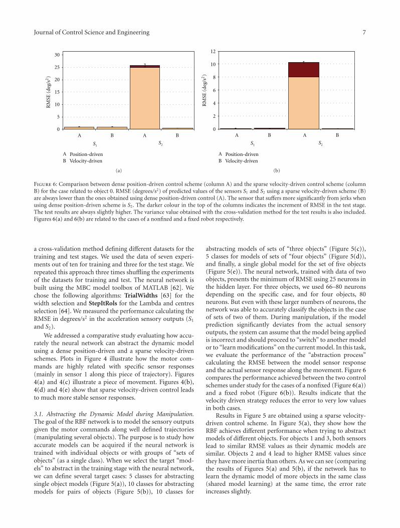
Journal of Control Science and Engineering 7
30
25
20
15
10
5
0
RM
SE (
deg/
s2)
A B A
A
B
BPosition-drivenVelocity-driven
S1S2
(a)
A B
12
10
8
6
4
2
0
RM
SE (
deg/
s2)
A B
AB
Position-drivenVelocity-driven
S1 S2
(b)
Figure 6: Comparison between dense position-driven control scheme (column A) and the sparse velocity-driven control scheme (columnB) for the case related to object 0. RMSE (degrees/s2) of predicted values of the sensors S1 and S2 using a sparse velocity-driven scheme (B)are always lower than the ones obtained using dense position-driven control (A). The sensor that suffers more significantly from jerks whenusing dense position-driven scheme is S2. The darker colour in the top of the columns indicates the increment of RMSE in the test stage.The test results are always slightly higher. The variance value obtained with the cross-validation method for the test results is also included.Figures 6(a) and 6(b) are related to the cases of a nonfixed and a fixed robot respectively.
a cross-validation method defining different datasets for thetraining and test stages. We used the data of seven experi-ments out of ten for training and three for the test stage. Werepeated this approach three times shuffling the experimentsof the datasets for training and test. The neural network isbuilt using the MBC model toolbox of MATLAB [62]. Wechose the following algorithms: TrialWidths [63] for thewidth selection and StepItRols for the Lambda and centresselection [64]. We measured the performance calculating theRMSE in degrees/s2 in the acceleration sensory outputs (S1
and S2).
We addressed a comparative study evaluating how accu-rately the neural network can abstract the dynamic modelusing a dense position-driven and a sparse velocity-drivenschemes. Plots in Figure 4 illustrate how the motor com-mands are highly related with specific sensor responses(mainly in sensor 1 along this piece of trajectory). Figures4(a) and 4(c) illustrate a piece of movement. Figures 4(b),4(d) and 4(e) show that sparse velocity-driven control leadsto much more stable sensor responses.
3.1. Abstracting the Dynamic Model during Manipulation.The goal of the RBF network is to model the sensory outputsgiven the motor commands along well defined trajectories(manipulating several objects). The purpose is to study howaccurate models can be acquired if the neural network istrained with individual objects or with groups of “sets ofobjects” (as a single class). When we select the target “mod-els” to abstract in the training stage with the neural network,we can define several target cases: 5 classes for abstractingsingle object models (Figure 5(a)), 10 classes for abstractingmodels for pairs of objects (Figure 5(b)), 10 classes for
abstracting models of sets of “three objects” (Figure 5(c)),5 classes for models of sets of “four objects” (Figure 5(d)),and finally, a single global model for the set of five objects(Figure 5(e)). The neural network, trained with data of twoobjects, presents the minimum of RMSE using 25 neurons inthe hidden layer. For three objects, we used 66–80 neuronsdepending on the specific case, and for four objects, 80neurons. But even with these larger numbers of neurons, thenetwork was able to accurately classify the objects in the caseof sets of two of them. During manipulation, if the modelprediction significantly deviates from the actual sensoryoutputs, the system can assume that the model being appliedis incorrect and should proceed to “switch” to another modelor to “learn modifications” on the current model. In this task,we evaluate the performance of the “abstraction process”calculating the RMSE between the model sensor responseand the actual sensor response along the movement. Figure 6compares the performance achieved between the two controlschemes under study for the cases of a nonfixed (Figure 6(a))and a fixed robot (Figure 6(b)). Results indicate that thevelocity driven strategy reduces the error to very low valuesin both cases.
Results in Figure 5 are obtained using a sparse velocity-driven control scheme. In Figure 5(a), they show how theRBF achieves different performance when trying to abstractmodels of different objects. For objects 1 and 3, both sensorslead to similar RMSE values as their dynamic models aresimilar. Objects 2 and 4 lead to higher RMSE values sincethey have more inertia than others. As we can see (comparingthe results of Figures 5(a) and 5(b), if the network has tolearn the dynamic model of more objects in the same class(shared model learning) at the same time, the error rateincreases slightly.

8 Journal of Control Science and Engineering
0
10.5
−1.5−1
−0.5
Th
resh
old-
RM
SE
(OB
J)
(a)
2 OBJ 3 OBJ 5 OBJ 4 OBJ0
0.51
1.5
2.52
Th
resh
old-
RM
SE
(OB
J)
0 3
0 1 2 4b
0 2 3 4a 0 1 3 4a 1 2 3 4
0 2 3 4b 0 1 3 4b
1 4
1 3
0 2 2 3
0 1 2 4a 1 2
0 1
2 4
3 4
0 3 4a
0 3 4b
1 2 3
1 2 4a
1 2 4b
1 3 4a
1 3 4b
0 1 2 0 1 3a
0 1 3b
0 1 4a
0 1 4b
0 2 3a
0 2 3b
0 2 4
2 3 4
0 1 2 3
0 4
0 1 2 3 4
(b)
Figure 7: Bars represent the object discrimination power of thenetwork (RBF) for all combinations of two, three, four, or fiveobjects respectively (see paragraph 3 for object classification). If theRMSE (OBJ) value of the label output for a specific set of objectslies below the discrimination threshold, an accurate classificationof objects can be achieved. Graphs show the result obtained with anon-fixed robot (Figure 7(a)) and with a fixed robot (Figure 7(b)),and each bar is associated to a combination of objects listed inthe legend from left to right, respectively. A combination with twothresholds (i.e., 0 3 4) has two bars and two labels (0 3 4a and 0 34b) and bars are joined together in the graph.
3.2. Classifying Objects during Manipulation. In Figure 7,the discrimination power of the RBF based on the dynamicmodel itself is shown. In this case, we evaluate if the RBFis able to accurately distinguish among different objectsassigning the correct labels (0, 1, 2, 3, and 4) by using only theinputs of the network (i.e., sensorimotor vectors). Evaluationof the classification performance is not straightforward andis based on the difference between the “discriminationthreshold” (half of the distance between the closest targetlabel values) and the RMSE value of the label output for aspecific set of objects. We have chosen a single dimensiondistribution of the classes, therefore, distances between thedifferent class labels are diverse. For instance, the “distance”between labels one and two is one, while the distance betweenlabels one and four is three and the threshold is the half ofthat distance. For any set of two or five objects (i.e. A (0 and1), B (1 and 3), and C (0, 1, 2, 3, and 4)) only one thresholdvalue exists (Th(A) = 0.5, Th(B) = 1, and Th(C) = [0.5, 0.5,0.5, 0.5]), while sets of three or four objects (i.e., D (1, 2,and 3), E (0, 2, and 3), and F (0, 1, 2, and 4), and G (1, 2, 3,and 4)) may have two threshold values (Th(D) = [0.5, 0.5],Th(E) = [1, 0.5], Th(F) = [0.5, 0.5, 1], and Th(G) = [0.5, 0.5,0.5]). We see that the RBF is able to correctly classify theobjects when using only two of them (values above zero)
RM
SE
3 OBJ 2 OBJ 4 OBJ 5 OBJ
1.6
1
00.20.40.60.8
1.21.4
1.8
Figure 8: Mean of RMSE for objects (OBJ) using the sparse veloci-ty-driven control scheme.
but the system becomes unreliable (negative values) whenusing three objects or more in the case of a standing robot(Figure 7(a)), while the RBF always correctly classifies theobjects when the robot is fixed to the ground (Figure 7(b)).
3.3. Accurate Manipulation Strategy: Classification with Cus-tom Control. We have abstracted dynamic models from ob-jects and can use them for accurate control (Figure 9).
(a) Direct Control. We control different objects directly. Dur-ing manipulation, the sensor responses are compared witha “shared model” to evaluate the performance. We measurethe RMSE comparing the global model output (model of thesensor outputs of two different manipulated objects) and theactual sensor outputs.
(b) Classification with Control. Since we are able to accuratelydistinguish between two objects (Figure 7(a)), we select thecorresponding individual model from the RBF network (seeFigure 3(a)) to obtain the acceleration values of the objectbeing manipulated instead of using a shared model with thedata of the two objects. In fact, the individual models ofthe five objects were previously learnt. The RMSE is alwayslower when single object models are used (Figure 9) (afteran object classification stage). Direct control using a global(shared) model achieves a lower performance because theapplied model does not take into account the singularitiesof each of the individual models.
The classification with control scheme is feasible whendealing with objects easy to be discriminated and the actualtrajectory of the movement follows more reliably the singleobject model than a “shared model.” In Figure 9, the RMSEis plotted when comparing sensor model response and theactual sensor responses. Figure 8 shows the accuracy of theclassification task when training the network with differentnumbers of objects (classification errors along the trajec-tory). Nevertheless, we have shown (Figure 7) that with theobjects used in our study, the network can only reliablyclassify the object (along the whole trajectory) when we focuson distinguishing between two objects.
4. Conclusions
The first conclusion of the presented work is that the appliedcontrol scheme is critical to facilitate reliable dynamic modelabstraction. In fact, the dynamic models or computed

Journal of Control Science and Engineering 9
RM
SE (
deg/
s2) 1.2
10.80.60.40.2
0A B C D E F G H I J
S1
(a)
0.70.8
0.60.50.40.30.20.1
0
Direct controlClassification + control
A B C D E F G H I J
RM
SE (
deg/
s2)
S2
(b)
Figure 9: Comparison between the individual and the shared models related to predicted sensory values S1 and S2. The columns of a lightercolour indicate RMSE for the direct control while the columns of a darker colour represent RMSE for the controller of a single object onceit is accurately classified. Cases (objects): A (0 and 1), B (0 and 2), C (0 and 3), D (0 and 4), E (1 and 2), F (1 and 3), G (1 and 4), H (2 and3), I (2 and 4), and J (3 and 4).
torques are used for high performance and compliant robotcontrol in terms of precision and energy efficiency [3, 65].
We have compared a dense position-driven versus asparse velocity-driven control strategy. The second schemeleads to smoother movements when manipulating differentobjects. This produces more stable sensor responses whichallow to model the dynamics of the movement. As modelabstraction engine, we have used a well-known RBF network(widely used for function approximation tasks) and wecompared its performance for abstracting dynamics modelsof the different objects using a sparse velocity-driven scheme(Figure 5(a)).
In a second part of the work, we have evaluated if theobject classification is feasible. More concretely, we havechecked out if we can perform it using sensorimotor com-plexes (motor commands, velocities, and local accelerations)obtained during object manipulation (exploration task) asinputs. Figure 7(a) shows that only the discrimination be-tween any pair of two objects was possible. Robots with lowgains will produce different actual movements when manip-ulating different objects, because these objects affect signif-icantly their dynamic model. If the robot is controlled withhigh gains, the differences in the dynamic model of the robotare compensated by the high control gains. If the robot istightly fixed but is controlled with low gains the actualmovement (sensorimotor representation of an object manip-ulation) is different for each object (Figure 7(b)). If the robotis slightly fixed, the control commands produce vibrationsthat perturb the dynamic model and, therefore, the differentsensorimotor representations are highly affected by thesenoisy artefacts (motor command driven vibrations) (seeFigure 7(a)).
Finally, by assuming that we are able to classify objectsduring manipulation and to switch to the best dynamicmodel, we have evaluated the accuracy when comparing themovement’s actual dynamics (actual sensor responses) withthe abstracted ones. Furthermore, we have evaluated the gainin performance if we compare it with a specific dynamicmodel instead of a “global” dynamics model. We have eval-uated the impact of this two-step control strategy obtainingan improvement of 30% (Figure 9) in predicting the sensoroutputs along the trajectory. This abstracted model can
be used in predicted control strategies or for stabilisationpurposes.
Summarising, our results prove that the presented robotand artificial neural network can abstract dynamic modelsof objects within the stream sensorimotor primitives duringmanipulation tasks. One of the most important results of thework shown in Figures 6(a) (nonfixed robot) and 6(b) (fixedrobot) indicates that robot platforms can highly benefitfrom nonrigid sparse velocity-driven control scheme. Thehigh error obtained with the dense position-driven controlscheme (Figure 6(a)) is caused by vibrations as the slightfixation of the robot to the ground is only supported by itsown weight. Furthermore, when we try to abstract a move-ment model, the performance achieved by the neural net-work (RBF) also represents a measurement of the stability ofthe movements (the repeatability of such trajectories whenapplying different control schemes).
Acknowledgments
This work has been supported in part by the EU GrantSENSOPAC (FP6-IST-028056) and by the Spanish NationalGrants DPI-2004-07032 and TEC2010-15396.
References
[1] H. Hoffmann, S. Schaal, and S. Vijayakumar, “Local dimen-sionality reduction for non-parametric regression,” NeuralProcessing Letters, vol. 29, no. 2, pp. 109–131, 2009.
[2] D. Nguyen-Tuong and J. Peters, “Learning robot dynamicsfor computed torque control using local Gaussian processesregression,” in Proceedings of the ECSIS Symposium on Learn-ing and Adaptive Behaviors for Robotic Systems (LAB-RS ’08),pp. 59–64, Edinburgh, UK, August 2008.
[3] G. Petkos, M. Toussaint, and S. Vijayakumar, “Learning mul-tiple models of nonlinear dynamics for control under varyingcontexts,” in Proceedings of the International Conference onArtificial Neural Networks (ICANN ’06), pp. 898–907, Athens,Greece, 2006.
[4] S. Vijayakumar, A. D’Souza, and S. Schaal, “Incrementalonline learning in high dimensions,” Neural Computation, vol.17, no. 12, pp. 2602–2634, 2005.

10 Journal of Control Science and Engineering
[5] S. Vijayakumar, A. D’souza, T. Shibata, J. Conradt, and S.Schaal, “Statistical learning for humanoid robots,” Autono-mous Robots, vol. 12, no. 1, pp. 55–69, 2002.
[6] R. Miall, “Motor control, biological and theoretical,” in Hand-book of Brain Theory and Neural Network, M. Arbib, Ed., pp.686–689, Bradford Books/MIT Press, Cambridge, Mass, USA,2nd edition, 2003.
[7] S. Schaal and N. Schweighofer, “Computational motor controlin humans and robots,” Current Opinion in Neurobiology, vol.15, no. 6, pp. 675–682, 2005.
[8] Sensopac, Eu project(SENSOrimotor structuring of Percep-tion and Action for emergent Cognition), 2010, http://www.sensopac.org/.
[9] C. Q. Huang, S. J. Shi, X. G. Wang, and W. K. Chung, “Par-allel force/position controllers for robot manipulators withuncertain kinematics,” International Journal of Robotics andAutomation, vol. 20, no. 3, pp. 158–167, 2005.
[10] J. Roy and L. L. Whitcomb, “Adaptive force control of position/velocity controlled robots: theory and experiment,” IEEETransactions on Robotics and Automation, vol. 18, no. 2, pp.121–137, 2002.
[11] M. Kawato, “Internal models for motor control and trajectoryplanning,” Current Opinion in Neurobiology, vol. 9, no. 6, pp.718–727, 1999.
[12] D. M. Wolpert and M. Kawato, “Multiple paired forward andinverse models for motor control,” Neural Networks, vol. 11,no. 7-8, pp. 1317–1329, 1998.
[13] D. H. Shin and A. Ollero, “Mobile robot path planning forfine-grained and smooth path specifications,” Journal of Ro-botic Systems, vol. 12, no. 7, pp. 491–503, 1995.
[14] M. H. Raibert and J. J. Craig, “Hybrid position/force controlof manipulators,” ASME Journal of Dynamic Systems, Measure-ment and Control, vol. 103, no. 2, pp. 126–133, 1981.
[15] M. W. Spong, S. Hutchinson, and M. Vidyasagar, RobotModeling and Control, John Wiley & Sons, New York, NY, USA,2006.
[16] W. Yu and M. A. Moreno-Armendariz, “Robust visual servo-ing of robot manipulators with neuro compensation,” Journalof the Franklin Institute, vol. 342, no. 7, pp. 824–838, 2005.
[17] W. Yu and X. Li, “PD control of robot with velocity estimationand uncertainties compensation,” International Journal ofRobotics and Automation, vol. 21, no. 1, pp. 1–9, 2006.
[18] J. J. de Rubio and L. A. Soriano, “An asymptotic stable pro-portional derivative control with sliding mode gravity com-pensation and with a high gain observer for robotic arms,”International Journal of Innovative Computing, Informationand Control, vol. 6, no. 10, pp. 4513–4525, 2010.
[19] J. de Jesus Rubio, C. Torres, and C. Aguilar, “Optimal controlbased in a mathematical model applied to robotic arms,” In-ternational Journal of Innovative Computing, Information andControl, vol. 7, no. 8, pp. 5045–5062, 2011.
[20] M. Haruno, D. M. Wolpert, and M. Kawato, “MOSAIC modelfor sensorimotor learning and control,” Neural Computation,vol. 13, no. 10, pp. 2201–2220, 2001.
[21] B. Daya, “Multilayer perceptrons model for the stability of abipedal robot,” Neural Processing Letters, vol. 9, no. 3, pp. 221–227, 1999.
[22] S. Tolu, E. Ros, and R. Agıs, “Bio-inspired control model forobject manipulation by humanoid robots,” in Proceedings ofthe Proceedings of the 9th international work conference onArtificial neural networks (IWANN ’07), pp. 822–829, SanSebastian, Spain, June 2007.
[23] R. R. Carrillo, E. Ros, C. Boucheny, and O. J. M. D. Coenen,“A real-time spiking cerebellum model for learning robotcontrol,” BioSystems, vol. 94, no. 1-2, pp. 18–27, 2008.
[24] N. R. Luque, J. A. Garrido, R. R. Carrillo, O. J.-M. D. Coenen,and E. Ros, “Cerebellar input configuration toward objectmodel abstraction in manipulation tasks,” IEEE Transactionson Neural Networks, vol. 22, no. 8, pp. 1321–1328, 2011.
[25] N. R. Luque, J. A. Garrido, R. R. Carrillo, O. J.-M. D. Coenen,and E. Ros, “Cerebellarlike corrective model inference enginefor manipulation tasks,” IEEE Transactions on Systems, Man,and Cybernetics B, vol. 41, no. 5, pp. 1299–1312, 2011.
[26] N. R. Luque, J. A. Garrido, R. R. Carrillo, S. Tolu, and E.Ros, “Adaptive cerebellar spiking model embedded in thecontrol loop: context switching and robustness against noise,”International Journal of Neural Systems, vol. 21, no. 5, pp. 385–401, 2011.
[27] M. H. Hassoun, Fundamentals of Artificial Neural Networks,Massachusetts Institute of Technology, Cambridge, Mass,USA, 1995.
[28] K. J. Hunt, D. Sbarbaro, R. Zbikowski, and P. J. Gawthrop,“Neural networks for control systems—a survey,” Automatica,vol. 28, no. 6, pp. 1083–1112, 1992.
[29] J. Constantin, C. Nasr, and D. Hamad, “Control of a robotmanipulator and pendubot system using artificial neuralnetworks,” Robotica, vol. 23, no. 6, pp. 781–784, 2005.
[30] T. D’Silva and R. Miikkulainen, “Learning dynamic obstacleavoidance for a robot arm using neuroevolution,” Neural Proc-essing Letters, vol. 30, no. 1, pp. 59–69, 2009.
[31] C. C. Lee, P. C. Chung, J. R. Tsai, and C. I. Chang, “Robustradial basis function neural networks,” IEEE Transactions onSystems, Man, and Cybernetics B, vol. 29, no. 6, pp. 674–685,1999.
[32] C. Chez, In Principles of Neural Science, Prentice Hall, London,UK, 3rd edition, 1991.
[33] M. Ito, “Mechanisms of motor learning in the cerebellum,”Brain Research, vol. 886, no. 1-2, pp. 237–245, 2000.
[34] C. Assad, S. Trujillo, S. Dastoor, and L. Xu, “Cerebellar dy-namic state estimation for a biomorphic robot arm,” in Pro-ceedings of the International Conference on Systems, Man andCybernetics, pp. 877–882, Waikoloa, Hawaii, USA, October2005.
[35] M. Ito, “Control of mental activities by internal models in thecerebellum,” Nature Reviews Neuroscience, vol. 9, no. 4, pp.304–313, 2008.
[36] P. Van Der Smagt, “Cerebellar control of robot arms,”Connection Science, vol. 10, no. 3-4, pp. 301–320, 1998.
[37] R. C. Miall, J. G. Keating, M. Malkmus, and W. T. Thach,“Simple spike activity predicts occurrence of complex spikesin cerebellar Purkinje cells,” Nature neuroscience, vol. 1, no. 1,pp. 13–15, 1998.
[38] R. Apps and M. Garwicz, “Anatomical and physiologicalfoundations of cerebellar information processing,” NatureReviews Neuroscience, vol. 6, no. 4, pp. 297–311, 2005.
[39] Ikarus, “Acceleration sensors,” 2011, http://www.ikarus-mod-ellbau.de.
[40] V. J. Lumelsky, M. S. Shur, and S. Wagner, “Sensitive skin,”IEEE Sensors Journal, vol. 1, no. 1, pp. 41–51, 2001.
[41] C. J. Khoh and K. K. Tan, “Adaptive robust control for servomanipulators,” Neural Computing and Applications, vol. 12,no. 3-4, pp. 178–184, 2003.
[42] M. Zhihong, X. H. Yu, and H. R. Wu, “An RBF neural network-based adaptive control for SISO linearisable nonlinear sys-tems,” Neural Computing and Applications, vol. 7, no. 1, pp.71–77, 1998.
[43] Celoxica Inc, 2011, http://www.celoxica.com/.[44] Hitec Robotics Inc, 2011, http://www.robonova.de/store/
home.php.

Journal of Control Science and Engineering 11
[45] C. G. Atkeson, C. H. An, and J. M. Hollerbach, “Estimation ofinertial parameters of manipulator loads and links,” Interna-tional Journal of Robotics Research, vol. 5, no. 3, pp. 101–119,1986.
[46] D. Kubus, T. Kroger, and F. M. Wahl, “On-line rigid objectrecognition and pose estimation based on inertial parameters,”in Proceedings of the IEEE/RSJ International Conference onIntelligent Robots and Systems (IROS ’07), pp. 1402–1408, SanDiego, Calif, USA, November 2007.
[47] J. J. Craig, Introduction to Robotics: Mechanics and Control,Pearson/Prentice Hall, Upper Saddle River, NJ, USA, 3rd edi-tion, 2005.
[48] M. Krabbes, C. Doschner et al., “Modelling of robot dynamicsbased on a multidimensional rbf-like neural network,” inProceedings of the International Conference on Information In-telligence and Systems (ICIIS’99), pp. 180–187, Bethesda, Md,USA, October/November 1999.
[49] R. J. Shilling, Fundamentals of Robotics: Analysis and Control,Prentice Hall, Englewood Cliffs, NJ, USA, 1990.
[50] P. Angelov, “Fuzzily connected multimodel systems evolvingautonomously from data streams,” IEEE Transactions onSystems, Man, and Cybernetics B, vol. 41, no. 4, pp. 898–910,2011.
[51] P. Angelov and D. Filev, “Simpl eTS: a simplified method forlearning evolving Takagi-Sugeno fuzzy models,” in Proceedingsof the IEEE International Conference on Fuzzy Systems, pp.1068–1073, Reno, Nev, USA, May 2005.
[52] G. P. Liu, V. Kadirkamanathan, and S. A. Billings, “Variableneural networks for adaptive control of nonlinear systems,”IEEE Transactions on Systems, Man and Cybernetics C, vol. 29,no. 1, pp. 34–43, 1999.
[53] H. J. Rong, N. Sundararajan, G. B. Huang, and P. Saratchan-dran, “Sequential Adaptive Fuzzy Inference System (SAFIS)for nonlinear system identification and prediction,” Fuzzy Setsand Systems, vol. 157, no. 9, pp. 1260–1275, 2006.
[54] J. de Jesus Rubio, D. M. Vazquez, and J. Pacheco, “Back-propagation to train an evolving radial basis function neuralnetwork,” Evolving Systems, vol. 1, no. 3, pp. 173–180, 2010.
[55] J. J. Rubio, F. Ortiz-Rodriguez, C. Mariaca-Gaspar, and J.Tovar, “A method for online pattern recognition of abnormal-eye movements,” Neural Computing & Applications. In press.
[56] D. K. Wedding and A. Eltimsahy, “Flexible link control usingmultiple forward paths, multiple RBF neural networks in adirect control application,” in Proceedings of the IEEE Interna-tional Conference on Systems, Man and Cybernetics, pp. 2619–2624, Nashville, Tenn, USA, October 2000.
[57] Z. D. Wang, E. Nakano, and T. Takahashi, “Solving functiondistribution and behavior design problem for cooperativeobject handling by multiple mobile robots,” IEEE Transactionson Systems, Man, and Cybernetics A, vol. 33, no. 5, pp. 537–549,2003.
[58] J. Flanagan, K. Merritt, and R. Johansson, “Predictive mech-anisms and object representations used in object manipu-lation,” in Sensorimotor Control of Grasping: Physiology andPathophysiology, pp. 161–177, Cambridge University Press,Cambridge, UK, 2009.
[59] C. C. Pagano, J. M. Kinsella-Shaw, P. E. Cassidy, and M. T.Turvey, “Role of the inertia tensor in haptically perceivingwhere an object is grasped,” Journal of Experimental Psychol-ogy: Human Perception and Performance, vol. 20, no. 2, pp.276–285, 1994.
[60] J. S. Bay, “Fully autonomous active sensor-based explorationconcept for shape-sensing robots,” IEEE Transactions on Sys-tems, Man and Cybernetics, vol. 21, no. 4, pp. 850–860, 1991.
[61] G. Petkos and S. Vijayakumar, “Load estimation and con-trol using learned dynamics models,” in Proceedings of theIEEE/RSJ International Conference on Intelligent Robots andSystems (IROS ’07), pp. 1527–1532, San Diego, Calif, USA,November 2007.
[62] Mathworks Inc, 2011, http://www.mathworks.com/products/matlab.
[63] M. Orr, J. Hallam, K. Takezawa et al., “Combining regressiontrees and radial basis function networks,” International Journalof Neural Systems, vol. 10, no. 6, pp. 453–465, 2000.
[64] S. Chen, E. S. Chng, and K. Alkadhimi, “Regularized orthog-onal least squares algorithm for constructing radial basisfunction networks,” International Journal of Control, vol. 64,no. 5, pp. 829–837, 1996.
[65] D. Nguyeii-Tuoiig, M. Seeger, and J. Peters, “Computed torquecontrol with nonparametric regression models,” in Proceedingsof the American Control Conference (ACC ’08), pp. 212–217,Seattle, Wash, USA, June 2008.
Hindawi Publishing CorporationJournal of Control Science and EngineeringVolume 2012, Article ID 545731, 9 pagesdoi:10.1155/2012/545731
Research Article
An Output-Recurrent-Neural-Network-Based Iterative LearningControl for Unknown Nonlinear Dynamic Plants
Ying-Chung Wang and Chiang-Ju Chien
Department of Electronic Engineering, Huafan University, Shihding, New Taipei City 223, Taiwan
Correspondence should be addressed to Chiang-Ju Chien, [email protected]
Received 31 July 2011; Revised 9 November 2011; Accepted 1 December 2011
Academic Editor: Isaac Chairez
Copyright © 2012 Y.-C. Wang and C.-J. Chien. This is an open access article distributed under the Creative Commons AttributionLicense, which permits unrestricted use, distribution, and reproduction in any medium, provided the original work is properlycited.
We present a design method for iterative learning control system by using an output recurrent neural network (ORNN).Two ORNNs are employed to design the learning control structure. The first ORNN, which is called the output recurrentneural controller (ORNC), is used as an iterative learning controller to achieve the learning control objective. To guarantee theconvergence of learning error, some information of plant sensitivity is required to design a suitable adaptive law for the ORNC.Hence, a second ORNN, which is called the output recurrent neural identifier (ORNI), is used as an identifier to provide therequired information. All the weights of ORNC and ORNI will be tuned during the control iteration and identification process,respectively, in order to achieve a desired learning performance. The adaptive laws for the weights of ORNC and ORNI andthe analysis of learning performances are determined via a Lyapunov like analysis. It is shown that the identification error willasymptotically converge to zero and repetitive output tracking error will asymptotically converge to zero except the initial resettingerror.
1. Introduction
Iterative learning control (ILC) system has become one ofthe most effective control strategies in dealing with repeatedtracking control of nonlinear plants. The ILC systemimproves the control performance by a self-tuning process inthe traditional PID-type ILC algorithms for linear plants oraffine nonlinear plants with nonlinearities satisfying globalLipschitz continuous condition [1–3]. Recently, the ILCstrategies combined with other control methodologies suchas observer-based iterative learning control [4], adaptive iter-ative learning control [5], robust iterative learning control[6], or adaptive robust iterative learning control [7], havebeen widely studied in order to extend the applications tomore general class of nonlinear systems. However, more andmore restrictions are required in theory to develop theselearning controllers. Among these ILC algorithms, PID-type ILC algorithms are still attractive to engineers sincethey are simple and effective for real implementations andindustry applications. A main problem of the PID-typeILC algorithms is that a sufficient condition required to
guarantee learning stability and convergence will depend onplant’s input/output coupling function (matrix). In general,it is hard to design the learning gain if the nonlineardynamic plant is highly nonlinear and unknown. In orderto get the input/output coupling function (matrix), the ILCusing a neural or fuzzy system to solve the learning gainimplementation problem can be found in [8, 9]. A neuralnetwork or a fuzzy system was used to approximate theinverse of plant’s input/output coupling function (matrix).The inverse function (matrix) is claimed to be an optimalchoice of the learning gain from a convergent condition pointof view. As the nonlinear system is assumed to be unknown,some offline adaptive mechanisms are applied to updatethe network parameters in order to approximate the idealoptimal learning gain.
Actually, for control of unknown nonlinear systems,neural-network-based controller has become an importantstrategy in the past two decades. Multilayer neural networks,recurrent neural networks and dynamic neural network [10–16] were used for the design of adaptive controllers. Onthe other hand, fuzzy logic system, fuzzy neural network,

2 Journal of Control Science and Engineering
recurrent fuzzy neural networks and dynamic fuzzy neuralnetwork were also a popular tool for the design of adaptivecontrollers [17–22]. These concepts have also been applied tothe design of adaptive iterative learning control of nonlinearplants [23–25]. However, few ILC works were developedfor general unknown nonlinear plants, especially nonaffinenonlinear plants. As the authors can understand, a real-time recurrent network (RTRN) was developed in [26] forreal-time learning control of general unknown nonlinearplants. But unfortunately, their learning algorithm dependson the generalized inverse of weight matrix in the RTRN. Ifthe generalized inverse of weight matrix does not exist, thelearning control scheme is not implementable.
In this paper, we consider the design of an iterativelearning controller for a class of unknown nonlinear dynamicplants. Motivated by our previous work in [27], an improvedversion of an identifier-based iterative learning controlleris proposed by using an output recurrent neural network(ORNN). Two ORNNs are used to design an ORNN-basediterative learning control system. The proposed ORNN-based ILC system includes an ORNN controller (ORNC)and an ORNN identifier (ORNI). The ORNC is used asan iterative learning controller to achieve the repetitivetracking control objective. The weights of ORNC are tunedvia adaptive laws determined by a Lyapunov-like analysis.In order to realize the adaptive laws and guarantee theconvergence of learning error, some information of theunknown plant sensitivity is required for the design of adap-tive laws. Hence, the ORNI is then applied as an identifierto provide the required information from plant sensitivity.In a similar way, the weights of ORNI are tuned via someadaptive laws determined by a Lyapunov-like analysis. Bothof the proposed ORNC and ORNI update their networkweights along the control iteration and identification process,respectively. This ORNN-based ILC system can be used toexecute a repetitive control task of a general nonlinear plant.It is shown that the identification error will asymptoticallyconverge to zero and repetitive output tracking error willasymptotically converge to zero except the initial resettingerror.
This paper is organized as follows. The structure ofORNN is introduced in Section 2. In Section 3, we presentthe design of ORNC and ORNI for the ORNN-based ILCsystem. The adaptation laws are derived and the learning per-formance is guaranteed based on a Lyapunov-like analysis.To illustrate the effectiveness of the proposed ILC system,a numerical example is used in Section 4 for computersimulation. Finally a conclusion is made in Section 5.
In the subsequent discussions, the following notationswill be used in all the sections.
(i) |z| denotes the absolute value of a function z.
(ii) ‖v‖ = √(vv) denotes the usual Euclidean norm of avector v = [v1, . . . , vn] ∈ Rn.
(iii) ‖A‖ = max1≤i≤n{∑m
j=1 |ai j|} denotes the norm of amatrix A = {ai j} ∈ Rn×m.
· · · · · · · · ·
· · ·Layer 1(input layer)
Layer 2(hidden layer)
Layer 3(output layer)
D
O(3)(t)
x1(t) xn(t)
Figure 1: Structure of the ORNN.
2. The Output Recurrent Neural Network
In this paper, two ORNNs are used to design an iterativelearning control system. The structure of the ORNN is shownin Figure 1, which comprises an input layer, a hidden layer,and an output layer.
(i) Layer 1 (Input Layer): Each node in this layerrepresents an input variable, which only transmitsinput value to the next layer directly. For the ith inputnode, i = 1, . . . ,n + 1,
net(1)i =
⎧⎨⎩xi, i = 1, . . . ,n
D[O(3)
], i = n + 1
O(1)i = f (1)
i
(net(1)
i
)= net(1)
i ,
(1)
where xi, i = 1, . . . ,n represents the ith external inputsignal to the ith node of layer 1, and D[O(3)] denotesthe delay of ORNN output O(3) whcih can be furtherdefined as xn+1 = D[O(3)].
(ii) Layer 2 (Hidden Layer): Each node in this layerperforms an activation function whose inputs comefrom input layer. For the �th hidden node, a sigmoidfunction is adopted here such that the �th node, � =1, . . . ,M will be represented as
net(2)� =
n+1∑i=1
Vi�x(2)i ,
O(2)� = f (2)
�
(net(2)
�
)= 1
1 + exp(−net(2)
�
) ,(2)
where x(2)i = O(1)
i , Vi� is the connective weightbetween the input layer and the hidden layer, M isthe number of neuron in the hidden layer.

Journal of Control Science and Engineering 3
(iii) Layer 3 (Output Layer): Each node in this layerrepresents an output node, which computes theoverall output as the summation of all input signalsfrom hidden layer. For the output node,
net(3) =M∑�=1
w� · x(3)� ,
O(3) = f (3)(
net(3))= net(3),
(3)
where x(3)� = O(2)
� and w� is the connective weightbetween the hidden layer and the output layer.
Let n denotes the dimension of input vector X =[x1, . . . , xn] ∈ Rn×1 of nonlinear function f (X) and Mdenotes the number of neurons in the hidden layer, theORNN which performs as an approximator of the nonlinearfunction f (X) is now described in a matrix form as follows:
O(3)(
D[O(3)
],X ,W ,V
)=WO(2)(VXa), (4)
where W ∈ RM×1 and V ∈ R(n+1)×M are output-hidden wight matrix and hidden-input weight matrix,respectively, X ∈ Rn×1 is the external input vector,Xa ≡ [X, D[O(3)]]
∈ R(n+1)×1 is the augmented neuralinput vector, and D[O(3)] denotes the delay of ORNNoutput O(3). The activation function vector is defined as
O(2)(VXa) ≡ [O(2)1 (V
1 Xa), . . . ,O(2)M (V
MXa)] ∈ RM×1
whereV = [V1,V2, . . . ,VM] withV� ∈ R(n+1)×1 being the �th
column vector, and O(2)� (V
� Xa) ≡ 1/(1 + exp(−V� Xa)) ∈ R,
� = 1, . . . ,M is a sigmoid function.
3. Design of Output-Recurrent-Neural- Network-Based IterativeLearning Control System
In this paper, we consider an unknown nonlinear dynamicplant which can perform a given task repeatedly over a finitetime sequence t = {0, . . . ,N} as follows:
y j(t + 1) = f(y j(t), . . . , y j(t − n + 1),uj(t)
), (5)
where j ∈ Z+ denotes the index of control iteration numberand t = {0, . . . ,N} denotes the time index. The signalsy j(t) and uj(t) ∈ R are the system output and input,respectively. f : Rn+1 → R is the unknown continuousfunction, n represents the respective output delay order.Given a specified desired trajectory yd(t), t ∈ {0, . . . ,N},the control objective is to design an output-recurrent-neural-network-based iterative learning control system such thatwhen control iteration number j is large enough, |yd(t) −y j(t)| will converge to some small positive error tolerancebounds for all t ∈ {0, . . . ,N} even if there exists an initialresetting error. Here the initial resetting error means thatyd(0) /= y j(0) for all j ≥ 1. To achieve the control objective,an iterative learning control system based on ORNN designis proposed in Figure 2. In this figure, D denotes the delay intime domain andM denotes the memory in control iterationdomain.
r(t)
ORNC
M
D
ORNI
A.L.
A.L.
Dynamicplant
Reference model
+−
uj(t) y j(t + 1)
uj−1(t)
y j(t)
yd(t + 1)
•
+−
sgn(yju(t))
yu, max(t)
ejc (t +1)
yk(t + 1)
ekI (t +1)
Figure 2: Block diagram of the ORNN-based ILC system.
Before we state the design steps of the proposed controlstructure, some assumptions on the unknown nonlinearsystem and desired trajectories are given as follows.
(A1) The nonlinear dynamic plant is a relaxed systemwhose input uj(t) and output y j(t) are related byy j(t) = 0 for all t ∈ {−∞, . . . ,−1}.
(A2) There exists a bounded unknown upper bounding
function yu,max(t) = max∀ j|y ju(t)| such that 0 <
|y ju(t)| ≤ yu,max(t), where the factor yju(t) = ∂y j(t +
1)/∂uj(t) represents the sensitivity of the plant withrespect to its input.
(A3) The reference model is designed to generatethe bounded desired trajectory yd(t + 1) =fd(yd(t), . . . , yd(t − n + 1), r(t)), which is basedon a specified bounded reference input r(t) withfd : Rn+1 → R being a continuous function.
The design of the ORNN-based iterative learning controlsystem is divided into two parts.
3.1. Part 1: Design of ORNC and Corresponding AdaptiveLaws. Based on the assumptions on the nonlinear plant (5),
we define a tracking error ejc(t) at jth control iteration as
follows:
ejc(t) = yd(t)− y j(t). (6)
It is noted that there exist bounded constants εjc , j ∈ Z+ such
that the initial value of ejc(t) will satisfy
∣∣∣e jc(0)∣∣∣ = ε
jc . (7)
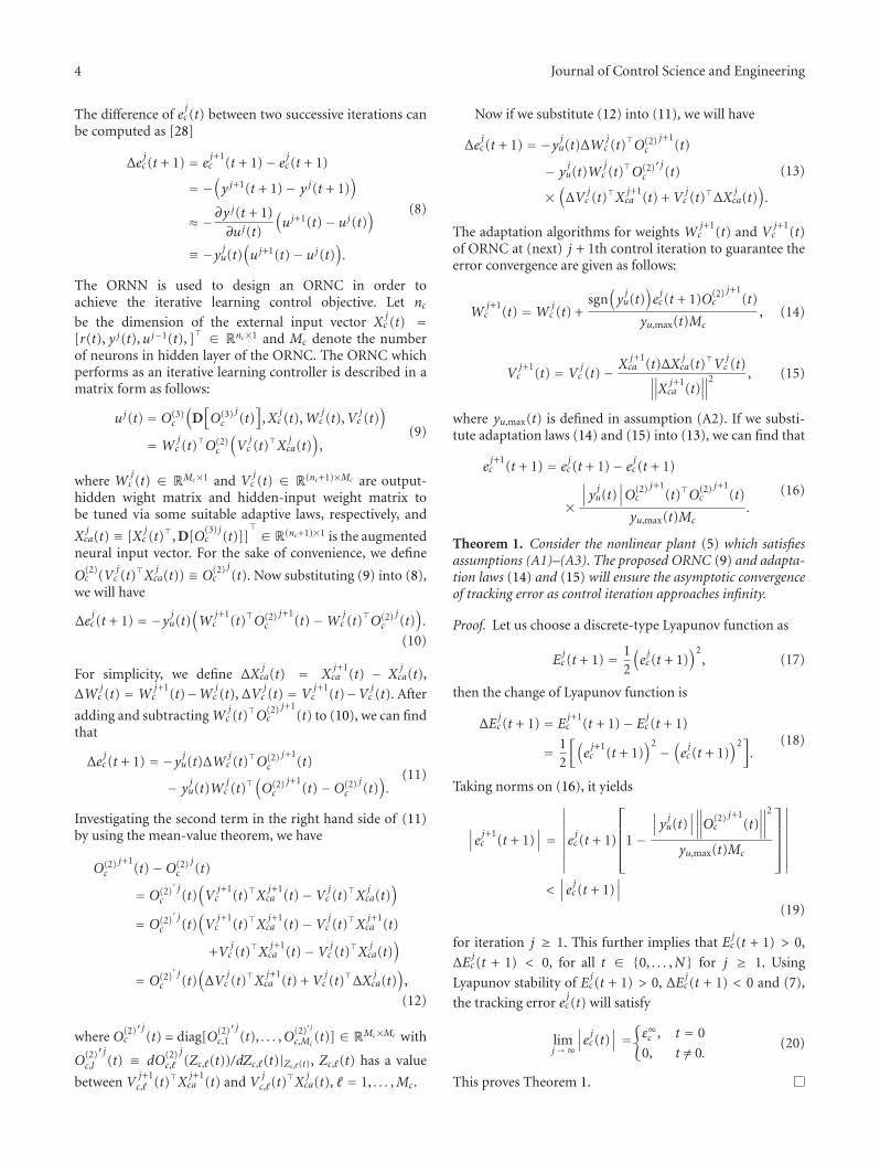
4 Journal of Control Science and Engineering
The difference of ejc(t) between two successive iterations can
be computed as [28]
Δejc(t + 1) = e
j+1c (t + 1)− e jc(t + 1)
= −(y j+1(t + 1)− y j(t + 1)
)≈ −∂y
j(t + 1)∂uj(t)
(uj+1(t)− uj(t)
)≡ −y ju(t)
(uj+1(t)− uj(t)
).
(8)
The ORNN is used to design an ORNC in order toachieve the iterative learning control objective. Let ncbe the dimension of the external input vector X
jc (t) =
[r(t), y j(t),uj−1(t), ] ∈ Rnc×1 and Mc denote the number
of neurons in hidden layer of the ORNC. The ORNC whichperforms as an iterative learning controller is described in amatrix form as follows:
uj(t) = O(3)c
(D[O(3)c
j(t)]
,Xjc (t),W
jc (t),V
jc (t)
)=W
jc (t)O(2)
c
(V
jc (t)X j
ca(t))
,(9)
where Wjc (t) ∈ RMc×1 and V
jc (t) ∈ R(nc+1)×Mc are output-
hidden wight matrix and hidden-input weight matrix tobe tuned via some suitable adaptive laws, respectively, and
Xjca(t) ≡ [X
jc (t), D[O
(3) jc (t)]]
∈ R(nc+1)×1 is the augmentedneural input vector. For the sake of convenience, we define
O(2)c (V
jc (t)X j
ca(t)) ≡ O(2)c
j(t). Now substituting (9) into (8),
we will have
Δejc(t + 1) = −y ju(t)
(W
j+1c (t)O(2)
cj+1
(t)−W jc (t)O(2)
cj(t)).
(10)
For simplicity, we define ΔXjca(t) = X
j+1ca (t) − X
jca(t),
ΔWjc (t) =W
j+1c (t)−W j
c (t), ΔVjc (t) = V
j+1c (t)−V j
c (t). After
adding and subtractingWjc (t)O(2)
cj+1
(t) to (10), we can findthat
Δejc(t + 1) = −y ju(t)ΔW
jc (t)O(2)
cj+1
(t)
− yju(t)W
jc (t)
(O(2)c
j+1(t)−O(2)
cj(t)).
(11)
Investigating the second term in the right hand side of (11)by using the mean-value theorem, we have
O(2)c
j+1(t)−O(2)
cj(t)
= O(2)c
′ j(t)(V
j+1c (t)X j+1
ca (t)−V jc (t)X j
ca(t))
= O(2)c
′ j(t)(V
j+1c (t)X j+1
ca (t)−V jc (t)X j+1
ca (t)
+Vjc (t)X j+1
ca (t)−V jc (t)X j
ca(t))
= O(2)c
′ j(t)(ΔV
jc (t)X j+1
ca (t) +Vjc (t)ΔX j
ca(t))
,
(12)
where O(2)c′ j
(t) = diag[O(2)c,1
′ j(t), . . . ,O(2)′ j
c,Mc(t)] ∈ RMc×Mc with
O(2)c,l
′ j(t) ≡ dO(2)
c,�
j(Zc,�(t))/dZc,�(t)|Zc,�(t), Zc,�(t) has a value
between Vj+1c,� (t)X j+1
ca (t) and Vjc,�(t)
X jca(t), � = 1, . . . ,Mc.
Now if we substitute (12) into (11), we will have
Δejc(t + 1) = −y ju(t)ΔW
jc (t)O(2)
cj+1
(t)
− yju(t)W
jc (t)O(2)
c′ j
(t)
×(ΔV
jc (t)X j+1
ca (t) +Vjc (t)ΔX j
ca(t)).
(13)
The adaptation algorithms for weights Wj+1c (t) and V
j+1c (t)
of ORNC at (next) j + 1th control iteration to guarantee theerror convergence are given as follows:
Wj+1c (t) =W
jc (t) +
sgn(yju(t)
)ejc(t + 1)O(2)
cj+1
(t)
yu,max(t)Mc, (14)
Vj+1c (t) = V
jc (t)− X
j+1ca (t)ΔX
jca(t)V j
c (t)∥∥∥X j+1ca (t)
∥∥∥2 , (15)
where yu,max(t) is defined in assumption (A2). If we substi-tute adaptation laws (14) and (15) into (13), we can find that
ej+1c (t + 1) = e
jc(t + 1)− e jc(t + 1)
×∣∣∣y ju(t)
∣∣∣O(2)c
j+1(t)O(2)
cj+1
(t)
yu,max(t)Mc.
(16)
Theorem 1. Consider the nonlinear plant (5) which satisfiesassumptions (A1)–(A3). The proposed ORNC (9) and adapta-tion laws (14) and (15) will ensure the asymptotic convergenceof tracking error as control iteration approaches infinity.
Proof. Let us choose a discrete-type Lyapunov function as
Ejc (t + 1) = 1
2
(ejc(t + 1)
)2, (17)
then the change of Lyapunov function is
ΔEjc (t + 1) = E
j+1c (t + 1)− E jc (t + 1)
= 12
[(ej+1c (t + 1)
)2 −(ejc(t + 1)
)2].
(18)
Taking norms on (16), it yields
∣∣∣e j+1c (t + 1)
∣∣∣ =∣∣∣∣∣∣∣∣∣e
jc(t + 1)
⎡⎢⎢⎢⎣1−
∣∣∣y ju(t)∣∣∣∥∥∥∥O(2)
cj+1
(t)∥∥∥∥2
yu,max(t)Mc
⎤⎥⎥⎥⎦∣∣∣∣∣∣∣∣∣
<∣∣∣e jc(t + 1)
∣∣∣(19)
for iteration j ≥ 1. This further implies that Ejc (t + 1) > 0,
ΔEjc (t + 1) < 0, for all t ∈ {0, . . . ,N} for j ≥ 1. Using
Lyapunov stability of Ejc (t + 1) > 0, ΔE
jc (t + 1) < 0 and (7),
the tracking error ejc(t) will satisfy
limj→∞
∣∣∣e jc(t)∣∣∣ ={ε∞c , t = 0
0, t /= 0.(20)
This proves Theorem 1.

Journal of Control Science and Engineering 5
Remark 2. If the plant sensitivity yju(t) is completely known
so that sgn(yju(t)) and yu,max(t) are available, then the control
objective can be achieved by using the adaptation algorithms
(14) and (15). However, the plant sensitivity yju(t) is in
general unknown or only partially known. In part 2, wewill design an ORNN-based identifier (ORNI) to estimate
the unknown plant sensitivity yju(t) and then provide the
sign function and upper bounding function of yju(t) for
adaptation algorithms of ORNC.
3.2. Part 2: Design of ORNI and Corresponding AdaptiveLaws. After each control iteration, the ORNI subsequentlybegins to perform identification process. The trained ORNIwill then provide the approximated plant sensitivity to theORNC to start the next control iteration. We would like toemphasize that the ORNI only identifies the nonlinear plantafter each control iteration. This concept is quite differentfrom traditional control tasks [29] and very important to theproposed ORNN-based ILC structure.
The structure of ORNN is further applied to design anORNI to identify the nonlinear plant after the jth controliteration. The identification process is stated as follows. Aftereach trial of controlling the nonlinear system, we collectthe input output data uj(t) and y j(t), t = 0, 1, . . . ,N +1 as the training data for the identifier. When discussingthe identification, we omit the control iteration index jand introduce a new identification iteration index k ∈Z+ to represent the number of identification process. Thatis, the notation for the training data uj(t), y j(t) and theORNI output y j,k(t) are simplified as u(t), y(t), and yk(t),respectively. For the ORNI, let nI be the dimension ofexternal input vector XI(t) = [u(t), y(t)] ∈ RnI×1 and MI
denote the number of neurons in hidden layer of the ORNI.The ORNI which performs as an iterative learning identifierfor nonlinear plant (5) is now described in a matrix form asfollows:
yk(t + 1) = O(3)I
(D[O(3)I
k(t)]
,XkIa(t),Wk
I (t),V kI (t)
)=Wk
I (t)O(2)I
(V kI (t)Xk
Ia(t))
,(21)
where WkI (t) ∈ RMI×1 and V k
I (t) ∈ R(nI+1)×MI are output-hidden wight matrix and hidden-input weight matrix tobe tuned via some suitable adaptive laws, respectively, and
XkIa(t) ≡ [XI(t)
, D[O(3)kI (t)]]
∈ R(nI+1)×1 is the augmentedneural input vector. For the sake of convenience, we define
O(2)I (V k
I (t)XkIa(t)) ≡ O(2)
I
k(t).
Based on the assumptions on the nonlinear plant (5),we define an identification error ekI (t) at kth identificationprocess as follows:
ekI (t) = y(t)− yk(t). (22)
The difference of ekI (t) between two successive identificationprocess can be computed as
ΔekI (t + 1) = ek+1I (t + 1)− ekI (t + 1)
= −(yk+1(t + 1)− yk(t + 1)
).
(23)
Now substituting (21) into (23), we will have
ΔekI (t + 1) = −(Wk+1
I (t)O(2)I
k+1(t)−Wk
I (t)O(2)I
k(t)).
(24)
For simplicity, we define ΔXkIa(t) = Xk+1
Ia (t) − XkIa(t),
ΔWkI (t) =Wk+1
I (t)−WkI (t), ΔV k
I (t) = V k+1I (t)−V k
I (t). After
adding and subtractingWkI (t)O(2)
I
k+1(t) to (24), we can find
ΔekI (t + 1) = −ΔWkI (t)O(2)
I
k+1(t)
−WkI (t)
(O(2)I
k+1(t)−O(2)
I
k(t)).
(25)
Investigating the second term in the right hand side of (25)by using the mean-value theorem, we can derive
O(2)I
k+1(t)−O(2)
I
k(t)
= O(2)I
′k(t)(V k+1I (t)Xk+1
Ia (t)−V kI (t)Xk
Ia(t))
= O(2)I
′k(t)(V k+1I (t)Xk+1
Ia (t)−V kI (t)Xk+1
Ia (t)
+V kI (t)Xk+1
Ia (t)−V kI (t)Xk
Ia(t))
= O(2)I
′k(t)(ΔV k
I (t)Xk+1Ia (t) +V k
I (t)ΔXkIa(t)
),
(26)
where O(2)I
′k(t) = diag[O(2)
I ,1
′k(t), . . . ,O(3)′k
I ,MI(t)] ∈ RMI×MI with
O(2)I ,�
′k(t) ≡ dO(2)
I ,�
k(ZI ,�(t))/dZI ,�(t)|ZI ,�(t), ZI ,�(t) has a value
between V k+1I ,� (t)Xk+1
Ia (t) and VjI ,�(t)
XkIa(t), � = 1, . . . ,MI .
Now if we substitute (26) into (25), we will have
ΔekI (t + 1) = −ΔWkI (t)O(2)
I
k+1(t)
−WkI (t)O(2)
I
′k(t)
×(ΔV k
I (t)Xk+1Ia (t) +V k
I (t)ΔXkIa(t)
).
(27)
The adaptation algorithms for weights Wk+1I (t) and
V k+1I (t) of ORNI at (next) k + 1th identification process are
given as follows:
Wk+1I (t) =Wk
I (t) +ekI (t + 1)O(2)
I
k+1(t)
MI
V k+1I (t) = V k
I (t)− Xk+1Ia (t)ΔXk
Ia(t)V kI (t)∥∥∥Xk+1
Ia (t)∥∥∥2 .
(28)
If we substitute adaptation laws (28) into (27), we have
ek+1I (t + 1) = ekI (t + 1)− ekI (t + 1)
O(2)I
k+1(t)O(2)
I
k+1(t)
MI.
(29)
Theorem 3. Consider the nonlinear dynamic plant (5) whichsatisfies assumptions (A1)–(A3). The proposed ORNI (21)and adaptation laws (28) will ensure that the asymptoticconvergence of identification error is guaranteed as the numbersof identification approach infinity.

6 Journal of Control Science and Engineering
Proof. Let us choose a discrete-type Lyapunov function as
EkI (t + 1) = 12
(ekI (t + 1)
)2, ∀t ∈ {0, . . . ,N}, (30)
then we can derive the change of Lyapunov function as
ΔEkI (t + 1) = Ek+1I (t + 1)− EkI (t + 1)
= 12
[(ek+1I (t + 1)
)2 −(ekI (t + 1)
)2].
(31)
Taking norms on (29), we have
∣∣∣ek+1I (t + 1)
∣∣∣ = ∣∣∣ekI (t + 1)∣∣∣∣∣∣∣∣∣∣∣∣1−
∥∥∥∥O(2)I
k+1(t)∥∥∥∥2
MI
∣∣∣∣∣∣∣∣∣<∣∣∣ekI (t + 1)
∣∣∣(32)
for iteration k ≥ 1. This implies that EkI (t + 1) > 0, ΔEkI (t +1) < 0, for all t ∈ {0, . . . ,N} for k ≥ 1, and hence theidentification error ekI (t) will satisfy limk→∞|ekI (t)| = 0, forall t ∈ {0, 1, . . . ,N}. This proves Theorem 3.
Remark 4. The ORNN is a promising tool for identificationbecause it can approximate any “well-behaved” nonlinearfunction to any desired accuracy. This good function approx-imation is applied to estimate the unknown plant sensitivity
in this paper. The plant sensitivity yju(t) in (8) can be
approximated as follows:
yju(t) ≡∂y
j(t + 1)∂uj(t)
≈ ∂ y j(t + 1)∂uj(t)
. (33)
Note that the index k in the identifier output yk(t) is removedonce the identification process stops. Applying the chain ruleto (21), it yields
∂ y j(t + 1)∂uj(t)
= ∂O(3)I
j(t)
∂uj(t)=
MI∑�=1
∂ y j(t + 1)
∂O(2)I ,�
j(t)
∂O(2)I ,�
j(t)
∂uj(t)
=MI∑�=1
wjI ,�(t)
∂O(2)I ,�
j(t)
∂uj(t).
(34)
Also from (21), we have
∂O(2)I ,�
j(t)
∂uj(t)= f (2)
I ,�
′(net(2)
I ,�
j(t))∂net(2)
I ,�
j(t)
∂uj(t). (35)
Since the inputs to ORNI are uj(t), y j(t) and D[O(3)I
j(t)],
we further have
net(2)I ,�
j(t) = V
jI ,1�(t)u
j(t) +VjI ,2�(t)y
j(t)
+VjI ,3�(t)D
[O(3)I
j(t)].
(36)
Thus,
∂net(2)I ,�
j(t)
∂uj(t)= V
jI ,1�(t). (37)
From (34), (35) and (37), we obtain
yju(t) = ∂ y j(t + 1)
∂uj(t)=
MI∑�=1
wjI ,�(t) f
(2)I ,�
′(net(2)
I ,�
j(t))V
jI ,1�(t),
(38)
where 0 < f (2)I ,�
′(net(2)
I ,�
j(t)) < 0.5. If we define ‖wj
I (t)‖ ≡max�|wj
I ,�(t)|, and ‖V jI ,1(t)‖ ≡ max�|V j
I ,1�(t)|, then
∣∣∣ y ju(t)∣∣∣ ≤MI
∥∥∥wjI (t)
∥∥∥∥∥∥∥ f (2)I ,�
′(net(2)
I ,�
j(t))V
jI ,1(t)
∥∥∥∥≤ MI
2
∥∥∥wjI (t)
∥∥∥∥∥∥V jI ,1(t)
∥∥∥ ≡ yju,max(t).
(39)
The sign function and upper bounding function of plantsensitivity after finishing the identification process at jthcontrol iteration can be obtained as follows:
sgn(yju(t)
)= sgn
(yju(t)
)yu,max(t) = max
{yju,max(t), y
j−1u,max(t)
}.
(40)
It is noted that we do not need the exact plant sensitivity yju(t)
for the design of adaptive law (14). Even though there may
exist certain approximation error between yju(t) and y
ju(t),
we can still guarantee the convergence of learning error sinceonly a upper bounding function is required. Also note that
the value of sgn(yju(t)) (+1 or −1) can be easily determined
from the identification result.
4. Simulation Example
In this section, we use the proposed ORNN-based ILCto iteratively control an unknown non-BIBO nonlineardynamic plant [26, 29]. The difference equation of thenonlinear dynamic plant is given as
y j(t + 1) = 0.2(y j(t)
)2+ 0.2y j(t − 1)
+ 0.4 sin(
0.5(y j(t − 1) + y j(t)
))× cos
(0.5(y j(t − 1) + y j(t)
))+ 1.2uj(t),
(41)
where y j(t) is the system output, uj(t) is the control input.The reference model is chosen as
yd(t + 1) = 0.6yd(t) + r(t), yd(0) = 0, (42)
where r(t) = sin(2πt/25) + sin(2πt/10) is a boundedreference input. The control objective is to force y j(t) totrack the desired trajectory yd(t) as close as possible over afinite time interval t ∈ {1, . . . , 200} except the initial point.The network weight adaptation for the ORNI and ORNCis designed according to (14), (15), and (28), respectively.
In the ORNC, we set Wjc (t) ∈ R2×1 and V
jc (t) ∈ R4×2,
that is, only two hidden nodes in layer 2 are used toconstruct the ORNC. In a similar way, we let Wk
I (t) ∈ R2×1
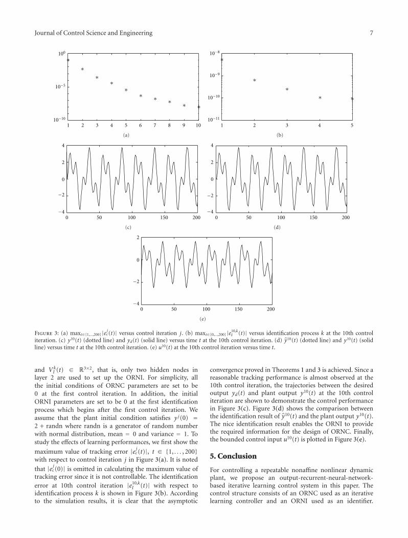
Journal of Control Science and Engineering 7
1 2 3 4 5 6 7 8 9 10
100
10−5
10−10
∗∗
∗∗
∗∗ ∗ ∗ ∗ ∗
(a)
1 2 3 4 5
10−8
10−9
10−10
10−11
∗
∗∗
∗ ∗
(b)
0 50 100 150 200
4
2
0
−2
−4
(c)
0 50 100 150 200
4
2
0
−2
−4
(d)
0 50 100 150 200
2
0
−2
−4
(e)
Figure 3: (a) maxt∈{1,...,200}|e jc (t)| versus control iteration j. (b) maxt∈{0,...,200}|e10,kI (t)| versus identification process k at the 10th control
iteration. (c) y10(t) (dotted line) and yd(t) (solid line) versus time t at the 10th control iteration. (d) y10(t) (dotted line) and y10(t) (solidline) versus time t at the 10th control iteration. (e) u10(t) at the 10th control iteration versus time t.
and V kI (t) ∈ R3×2, that is, only two hidden nodes in
layer 2 are used to set up the ORNI. For simplicity, allthe initial conditions of ORNC parameters are set to be0 at the first control iteration. In addition, the initialORNI parameters are set to be 0 at the first identificationprocess which begins after the first control iteration. Weassume that the plant initial condition satisfies y j(0) =2 + randn where randn is a generator of random numberwith normal distribution, mean = 0 and variance = 1. Tostudy the effects of learning performances, we first show the
maximum value of tracking error |e jc(t)|, t ∈ {1, . . . , 200}with respect to control iteration j in Figure 3(a). It is noted
that |e jc(0)| is omitted in calculating the maximum value oftracking error since it is not controllable. The identificationerror at 10th control iteration |e10,k
I (t)| with respect toidentification process k is shown in Figure 3(b). Accordingto the simulation results, it is clear that the asymptotic
convergence proved in Theorems 1 and 3 is achieved. Since areasonable tracking performance is almost observed at the10th control iteration, the trajectories between the desiredoutput yd(t) and plant output y10(t) at the 10th controliteration are shown to demonstrate the control performancein Figure 3(c). Figure 3(d) shows the comparison betweenthe identification result of y10(t) and the plant output y10(t).The nice identification result enables the ORNI to providethe required information for the design of ORNC. Finally,the bounded control input u10(t) is plotted in Figure 3(e).
5. Conclusion
For controlling a repeatable nonaffine nonlinear dynamicplant, we propose an output-recurrent-neural-network-based iterative learning control system in this paper. Thecontrol structure consists of an ORNC used as an iterativelearning controller and an ORNI used as an identifier.

8 Journal of Control Science and Engineering
The ORNC is the main controller utilized to achieve therepetitive control task. The ORNI is an auxiliary componentutilized to provide some useful information from plantsensitivity for the design of ORNC’s adaptive laws. All thenetwork weights of ORNC and ORNI will be tuned duringthe control iteration and identification process so that noprior plant knowledge is required. The adaptive laws for theweights of ORNC and ORNI and the analysis of learningperformances are determined via a Lyapunov-like analysis.We show that if the ORNI can provide the knowledge ofplant sensitivity for ORNC, then output tracking error willasymptotically converge to zero except an initial resettingerror. We also show that the objective of identification canbe achieved by the ORNI if the number of identifications islarge enough.
Acknowledgment
This work is supported by National Science Council, R.O.C.,under Grant NSC99-2221-E-211-011-MY2.
References
[1] K. L. Moore and J. X. Xu, “Special issue on iterative learningcontrol,” International Journal of Control, vol. 73, no. 10, pp.819–823, 2000.
[2] D. A. Bristow, M. Tharayil, and A. G. Alleyne, “A survey ofiterative learning,” IEEE Control Systems Magazine, vol. 26, no.3, pp. 96–114, 2006.
[3] H. S. Ahn, Y. Q. Chen, and K. L. Moore, “Iterative learningcontrol: brief survey and categorization,” IEEE Transactions onSystems, Man and Cybernetics. Part C, vol. 37, no. 6, pp. 1099–1121, 2007.
[4] J. X. Xu and J. Xu, “Observer based learning control fora class of nonlinear systems with time-varying parametricuncertainties,” IEEE Transactions on Automatic Control, vol.49, no. 2, pp. 275–281, 2004.
[5] I. Rotariu, M. Steinbuch, and R. Ellenbroek, “Adaptiveiterative learning control for high precision motion systems,”IEEE Transactions on Control Systems Technology, vol. 16, no.5, pp. 1075–1082, 2008.
[6] A. Tayebi, S. Abdul, M. B. Zaremba, and Y. Ye, “Robustiterative learning control design: application to a robotmanipulator,” IEEE/ASME Transactions on Mechatronics, vol.13, no. 5, pp. 608–613, 2008.
[7] J. X. Xu and B. Viswanathan, “Adaptive robust iterativelearning control with dead zone scheme,” Automatica, vol. 36,no. 1, pp. 91–99, 2000.
[8] J.Y. Choi and H. J. Park, “Neural-based iterative learningcontrol for unknown systems,” in Proceedings of the 2nd AsianControl Conference, pp. II243–II246, Seoul, Korea, 1997.
[9] C. J. Chien, “A sampled-data iterative learning control usingfuzzy network design,” International Journal of Control, vol. 73,no. 10, pp. 902–913, 2000.
[10] J. H. Park, S. H. Huh, S. H. Kim, S. J. Seo, and G. T. Park,“Direct adaptive controller for nonaffine nonlinear systemsusing self-structuring neural networks,” IEEE Transactions onNeural Networks, vol. 16, no. 2, pp. 414–422, 2005.
[11] J. S. Wang and Y. P. Chen, “A fully automated recurrentneural network for unknown dynamic system identification
and control,” IEEE Transactions on Circuits and Systems I, vol.53, no. 6, pp. 1363–1372, 2006.
[12] C. F. Hsu, C. M. Lin, and T. T. Lee, “Wavelet adaptivebackstepping control for a class of nonlinear systems,” IEEETransactions on Neural Networks, vol. 17, no. 5, pp. 1–9, 2006.
[13] C. M. Lin, L. Y. Chen, and C. H. Chen, “RCMAC hybridcontrol for MIMO uncertain nonlinear systems using sliding-mode technology,” IEEE Transactions on Neural Networks, vol.18, no. 3, pp. 708–720, 2007.
[14] Z. G. Hou, M. M. Gupta, P. N. Nikiforuk, M. Tan, and L.Cheng, “A recurrent neural network for hierarchical control ofinterconnected dynamic systems,” IEEE Transactions on NeuralNetworks, vol. 18, no. 2, pp. 466–481, 2007.
[15] Z. Liu, R. E. Torres, N. Patel, and Q. Wang, “Furtherdevelopment of input-to-state stabilizing control for dynamicneural network systems,” IEEE Transactions on Systems, Man,and Cybernetics Part A: Systems and Humans, vol. 38, no. 6, pp.1425–1433, 2008.
[16] Z. Liu, S. C. Shih, and Q. Wang, “Global robust stabilizing con-trol for a dynamic neural network system,” IEEE Transactionson Systems, Man, and Cybernetics Part A: Systems and Humans,vol. 39, no. 2, pp. 426–436, 2009.
[17] Y. G. Leu, W. Y. Wang, and T. T. Lee, “Observer-baseddirect adaptive fuzzy-neural control for nonaffine nonlinearsystems,” IEEE Transactions on Neural Networks, vol. 16, no. 4,pp. 853–861, 2005.
[18] S. Labiod and T. M. Guerra, “Adaptive fuzzy control of a classof SISO nonaffine nonlinear systems,” Fuzzy Sets and Systems,vol. 158, no. 10, pp. 1126–1137, 2007.
[19] B. Chen, X. Liu, and S. Tong, “Adaptive fuzzy outputtracking control of MIMO nonlinear uncertain systems,” IEEETransactions on Fuzzy Systems, vol. 15, no. 2, pp. 287–300,2007.
[20] Y. J. Liu and W. Wang, “Adaptive fuzzy control for a class ofuncertain nonaffne nonlinear system,” Information Sciences,vol. 177, no. 18, pp. 3901–3917, 2007.
[21] R. J. Wai and C. M. Liu, “Design of dynamic petri recurrentfuzzy neural network and its application to path-trackingcontrol of nonholonomic mobile robot,” IEEE Transactions onIndustrial Electronics, vol. 56, no. 7, pp. 2667–2683, 2009.
[22] C. H. Lee, Y. C. Lee, and F. Y. Chang, “A dynamic fuzzy neuralsystem design via hybridization of EM and PSO algorithms,”IAENG International Journal of Computer Science, vol. 37, no.3, 2010.
[23] W. G. Seo, B. H. Park, and J. S. Lee, “Adaptive fuzzy learningcontrol for a class of nonlinear dynamic systems,” InternationalJournal of Intelligent Systems, vol. 15, no. 12, pp. 1157–1175,2000.
[24] C. J. Chien and L. C. Fu, “Iterative learning control ofnonlinear systems using neural network design,” Asian Journalof Control, vol. 4, no. 1, pp. 21–29, 2002.
[25] C. J. Chien, “A combined adaptive law for fuzzy iterativelearning control of nonlinear systems with varying controltasks,” IEEE Transactions on Fuzzy Systems, vol. 16, no. 1, pp.40–51, 2008.
[26] T. W.S. Chow and Y. Fang, “A recurrent neural-network-based real-time learning control strategy applying to nonlinearsystems with unknown dynamics,” IEEE Transactions onIndustrial Electronics, vol. 45, no. 1, pp. 151–161, 1998.
[27] Y. C. Wang, C. J. Chien, and D. T. Lee, “An output recurrentfuzzy neural network based iterative learning control fornonlinear systems,” in Proceedings of the IEEE International

Journal of Control Science and Engineering 9
Conference on Fuzzy Systems, pp. 1563–1569, Hong Kong,2008.
[28] Y. C. Wang and C. C. Teng, “Output recurrent fuzzy neuralnetworks based model reference control for unknown nonlin-ear systems,” International Journal of Fuzzy Systems, vol. 6, no.1, pp. 28–37, 2004.
[29] C. C. Ku and K. Y. Lee, “Diagonal recurrent neural networksfor dynamic systems control,” IEEE Transactions on NeuralNetworks, vol. 6, no. 1, pp. 144–156, 1995.

Hindawi Publishing CorporationJournal of Control Science and EngineeringVolume 2012, Article ID 618403, 10 pagesdoi:10.1155/2012/618403
Research Article
3D Nonparametric Neural Identification
Rita Q. Fuentes,1 Isaac Chairez,2 Alexander Poznyak,1 and Tatyana Poznyak3
1 Automatic Control Department, CINVESTAV-IPN, 07360 Mexico, DF, Mexico2 Bioprocess Department, UPIBI-IPN, 07360 Mexico, DF, Mexico3 SEPI, ESIQIE-IPN, 07738 Mexico, DF, Mexico
Correspondence should be addressed to Rita Q. Fuentes, [email protected]
Received 23 August 2011; Accepted 2 October 2011
Academic Editor: Haibo He
Copyright © 2012 Rita Q. Fuentes et al. This is an open access article distributed under the Creative Commons AttributionLicense, which permits unrestricted use, distribution, and reproduction in any medium, provided the original work is properlycited.
This paper presents the state identification study of 3D partial differential equations (PDEs) using the differential neural networks(DNNs) approximation. There are so many physical situations in applied mathematics and engineering that can be described byPDEs; these models possess the disadvantage of having many sources of uncertainties around their mathematical representation.Moreover, to find the exact solutions of those uncertain PDEs is not a trivial task especially if the PDE is described in two or moredimensions. Given the continuous nature and the temporal evolution of these systems, differential neural networks are an attrac-tive option as nonparametric identifiers capable of estimating a 3D distributed model. The adaptive laws for weights ensure the“practical stability” of the DNN trajectories to the parabolic three-dimensional (3D) PDE states. To verify the qualitative behaviorof the suggested methodology, here a nonparametric modeling problem for a distributed parameter plant is analyzed.
1. Introduction
1.1. 3D Partial Differential Equations. Partial differentialequations (PDEs) are of vast importance in applied mathe-matics, physics, and engineering since so many real physicalsituations can be modelled by them. The dynamic descrip-tion of natural phenomenons are usually described by a setof differential equations using mathematical modeling rules[1]. Almost every system described in PDE has already ap-peared in the one- and two-dimensional situations. Append-ing a third dimension ascends the dimensional ladder to itsultimate rung, in physical space at least. For instance, lin-ear second-order 3D partial differential equations appear inmany problems modeling equilibrium configurations ofsolid bodies, the three-dimensional wave equation governingvibrations of solids, liquids, gases, and electromagneticwaves, and the three-dimensional heat equation modelingbasic spatial diffusion processes. These equations define astate representing rectangular coordinates on R3. There aresome basic underlying solution techniques to solve 3D PDEs:separation of variables and Green’s functions or fundamentalsolutions. Unfortunately, the most powerful of the planar
tools, conformal mapping, does not carry over to higher di-mensions. In this way, many numerical techniques solvingsuch PDE, for example, the finite difference method (FDM)and the finite element method (FEM), have been developed(see [2, 3]). The principal disadvantage of these methods isthat they require the complete mathematical knowledge ofthe system to define a mesh (domain discretization), wherethe functions are approximated locally. The construction of amesh in two or more dimensions is a nontrivial task. Usually,in practice, only low-order approximations are employed re-sulting in a continuous approximation of the function acrossthe mesh but not in its partial derivatives. The approximationdiscontinuities of the derivative can adversely affect the stab-ility of the solution. However, all those methods are well de-fined if the PDE structure is perfectly known. Actually, themost of suitable numerical solutions could be achieved onlyif the PDE is linear. Nevertheless, there are not so manymethods to solve or approximate the PDE solution when itsstructure (even in a linear case) is uncertain. This paper sug-gests a different numerical solution for uncertain systems(given by a 3D PDE) based on the Neural Network approach[4].

2 Journal of Control Science and Engineering
1.2. Application of Neural Networks to Model PDEs. Recentresults show that neural networks techniques seem to be veryeffective to identify a wide class or systems when we have nocomplete model information, or even when the plant is con-sidered as a gray box. It is well known that radial basis func-tion neural networks (RBFNNs) and MultiLayer Perceptrons(MLPs) are considered as a powerful tool to approximatenonlinear uncertain functions (see [5]): any continuous fun-ction defined on a compact set can be approximated to arbit-rary accuracy by such class of neural networks [6]. Since thesolutions of interesting PDEs are uniformly continuous andthe viable sets that arise in common problems are often com-pact, neural networks seem like ideal candidates for approxi-mating viability problems (see [7, 8]). Neural networks mayprovide exact approximation for PDE solutions; however,numerical constraints avoid this possible exactness because itis almost impossible to simulate NN structures with infinitenumber of nodes (see [7, 9, 10]). The Differential NeuralNetwork (DNN) approach avoids many problems related toglobal extremum search converting the learning process toan adequate feedback design (see [11, 12]). Lyapunov’s stabi-lity theory has been used within the neural networks frame-work (see [4, 11, 13]). The contributions given in this paperregard the development of a nonparametric identifier for 3Duncertain systems described by partial differential equations.The method produces an artificial mathematical model inthree dimensions that is able to describe the PDEs dynamics.The required numerical algorithm to solve the non-para-metric identifier was also developed.
2. 3D Finite Differences Approximation
The problem requires the proposal of a non-parametric iden-tifier based on DNN in three dimensions. The problem heremay be treated within the PDEs framework. Therefore, thissection introduces the DNN approximation characteristics toreconstruct the trajectories profiles for a family of 3D PDEs.
Consider the set of uncertain second-order PDEs
ut = f(u,ux,uxx,uy ,uyy ,uz,uzz,uxy ,uyx,uxz,uyz
)+ ξ, (1)
here uh = uh(x, y, z, t), where h represents t, x, y, z, xx, yy,zz, xy, xz, yx, yz and u = u(x, y, z, t) has n components(u(x, y, z, t) ∈ Rn) defined in a domain given by [x, y, z) ∈[0, 1]×[0, 1]×[0, 1], t ≥ 0, ξ = ξ(x, y, z, t) ∈ Rn is a noise inthe state dynamics. This PDE has a set of initial and boundaryconditions given by
ux(0, y, z, t
) = 0 ∈ Rn, u(x, 0, z, t) = u0 ∈ Rn,
u(x, y, 0, t
) = u0 ∈ Rn, u(x, y, z, 0
) = c ∈ Rn.(2)
In (1), ut(x, y, z, t) stands for ∂u(x, y, z, t)/∂t.System (1) armed with boundary and initial conditions
(2) is driven in a Hilbert spaceH equipped with an inner pro-duct (·, ·). Let us consider a vector function g(t) ∈ H to bea piecewise continuous in t. By L∞(a, b;H) we denote theset of H-valued functions g such that (g(·),u) is Lebesguemeasurable for all u ∈ H and essmaxt∈[a,b]‖g(γ, t)‖ < ∞,
γ ∈ Rn. Suppose that the nonlinear function g(γ, t) satisfiesthe Lipschitz condition ‖g(γ, t)− g(η, t)‖ ≤ L‖γ − η‖,
∀γ,η ∈ Br(γ0)
:= {γ ∈ Rn | ∥∥γ − γ0∥∥ ≤ r, ∀t ∈ [t0, t1]
},
(3)
where L is positive constant and ‖g‖2 = (g, g) is used just toensure that there exists some δ > 0 such that the state equa-tion γ = g(γ, t) with γ(t0) = γ0 has a unique solution over[t0, t0 + δ] (see [14]). The norm defined above stands for theSobolev space defined in [15] as follows.
Definition 1. Let Ω be an open set in Rn, and let ν ∈ Cm(Ω).Define the norm of ν(γ) as
‖ν‖m,p :=∑
0≤|α|≤m
(∫Ω
∣∣Dαν(γ)∣∣pdγ)1/p
(4)
(1 ≤ p < ∞, Dαν(γ) := (∂α/∂γα)ν(γ)). This is the Sobolevnorm in which the integration is performed in the Lebesguesense. The completion of the space of function ν(γ) ∈Cm(Ω): ‖ν‖m,p < ∞ with respect to ‖ · ‖m,p is the Sobolevspace Hm,p(Ω). For p = 2, the Sobolev space is a Hilbertspace (see [14, 15]).
Below we will use the norm (4) for the functions u(·, t)for each fixed t.
2.1. Numerical Approximation for Uncertain Functions. Nowconsider a function h0(·) in Hm,2(Ω). By [16], h0(·) can berewritten as
h0(γ, θ∗
) =∑i
∑j
∑k
θ∗i jkΨi jk(γ),
θi jk =∫ +∞
−∞h0(γ)Ψi jk
(γ)dγ, ∀i, j, k ∈ Z,
(5)
where {Ψi jk(γ)} are functions constituting a basis inHm,2(Ω). Last expression is referred to as a vector functionseries expansion of h0(γ, θ∗). Based on this series expansion,an NN takes the following mathematical structure:
h0(γ, θ
):=
L2∑i=L1
M2∑j=M1
N2∑k=N1
θi jkΨi jk(γ) = ΘTW
(γ)
(6)
that can be used to approximate a nonlinear functionh0(γ, θ∗) ∈ S with an adequate selection of integers L1, L2,M1, M2, N1, N2 ∈ Z+, where
Θ = [θL1M1N1 , . . . , θL1M1N2 , . . . θL2M1N1 , . . . θL2M2N2
]ᵀ,
W(γ) = [ΨL1M1N1 , . . . ,ΨL1M1N2 , . . .ΨL2M1N1 , . . .ΨL2M2N2
]ᵀ.
(7)
Following the Stone-Weierstrass Theorem [17], if
ε(L1,L2,M1,M2,N1,N2) = h0(γ, θ∗
)− h0(γ, θ
)(8)
is the NN approximation error, then for any arbitrary posi-tive constant ε there are some constants L1,L2,M1,M2,N1,N2 ∈ Z such that for all x ∈ X ⊂ R
‖ε(L1,L2,M1,M2,N1,N2)‖2 ≤ ε. (9)
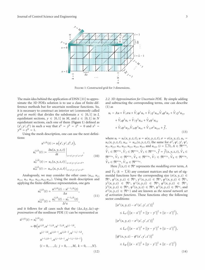
Journal of Control Science and Engineering 3
x = 0
y = 0
x = L
y =M
k=
1
k=N−
1
Δx
Δz
Δy
z=
0 i = 1
i = L− 1
N=z
· · ·
···
· ··
j =M −
1
j = 1
Figure 1: Constructed grid for 3 dimensions.
The main idea behind the application of DNN [11] to appro-ximate the 3D PDEs solution is to use a class of finite-dif-ference methods but for uncertain nonlinear functions. So,it is necessary to construct an interior set (commonly calledgrid or mesh) that divides the subdomain x ∈ [0, 1] in Lequidistant sections, y ∈ [0, 1] in M, and z ∈ [0, 1] in Nequidistant sections, each one of them (Figure 1) defined as(xi, y j , zk) in such a way that x0 = y0 = z0 = 0 and xL =yM = zN = 1.
Using the mesh description, one can use the next defini-tions:
ui, j,k(t) := u(xi, y j , zk, t
),
ui, j,kt (t) := ∂u
(x, y, z, t
)∂t
∣∣∣∣∣x=xi,y=y j ,z=zk
,
ui, j,kx (t) := ux
(x, y, z, t
)∣∣x=xi,y=y j ,z=zk ,
ui, j,kxx (t) := uxx
(x, y, z, t
)∣∣x=xi,y=y j ,z=zk .
(10)
Analogously, we may consider the other cases (uxx, uy ,uyy , uz, uzz, uxy ,uxz,uyz). Using the mesh description andapplying the finite-difference representation, one gets
ui, j,kx (t) � ui, j,k(t)− ui−1, j,k(t)
Δx,
ui, j,kxx (t) � u
i, j,kx (t)− ui−1, j,k
x (t)Δ2x
,
(11)
and it follows for all cases such that the (Δx,Δy,Δz)-ap-proximation of the nonlinear PDE (1) can be represented as
ui, j,k(t) = ui, j,kt (t)
� Φ(ui, j,k,ui−1, j,k,ui−2, j,k,ui, j−1,k,
ui, j−2,k,ui, j,k−1,ui, j,k−2,ui−1, j−1,k,
ui−1, j,k−1,ui, j−1,k−1,ui−1, j−1,k−1)
(i = 0, . . . ,L; j = 0, . . . ,M, k = 0, . . . ,N
).
(12)
2.2. 3D Approximation for Uncertain PDE. By simple addingand subtracting the corresponding terms, one can describe(1) as
ut = Au +◦V 1σu +
◦V 2ϕ
1ux +◦V 3γ
1uxx◦V 4ϕ
2uy +◦V 5γ
2uyy
+◦V 6ϕ
3uz +◦V 7γ
3uzz +◦V 8ψ
1uxy
+◦V 9ψ
2uyz◦V 10ψ
3uxz +◦V 11σ
2uxyz + f ,(13)
where ut = ut(x, y, z, t), u = u(x, y, z, t), σ = σ(x, y, z), ux =ux(x, y, z, t), uxx = uxx(x, y, z, t), the same for σ2, ϕi, γi, ψi,uy , uyy , uz, uzz, uxy , uyz, uxz, and uxyz (i = 1, 3), A ∈ Rn×n,◦V 1 ∈ Rn×s1 ,
◦V 2 ∈ Rn×s2 ,
◦V 3 ∈ Rn×s3 , f = f (x, y, z, t),
◦V 4 ∈
Rn×s4 ,◦V 5 ∈ Rn×s5 ,
◦V 6 ∈ Rn×s6 ,
◦V 7 ∈ Rn×s7 ,
◦V 8 ∈ Rn×s8 ,
◦V 9 ∈ Rn×s9 ,
◦V 10 ∈ Rn×s10 .
Here f (x, t) ∈ Rn represents the modelling error term, A
and◦V k (k = 1, 6) any constant matrices and the set of sig-
moidal functions have the corresponding size (σ(x, y, z) ∈Rs1 , ϕ1(x, y, z) ∈ Rs2 , γ1(x, y, z) ∈ Rs3 , ϕ2(x, y, z) ∈ Rs4 ,γ2(x, y, z) ∈ Rs5 , ψ1(x, y, z) ∈ Rs6 , ϕ3(x, y, z) ∈ Rs7 ,γ3(x, y, z) ∈ Rs8 , ψ2(x, y, z) ∈ Rs9 , ψ3(x, y, z) ∈ Rs10 , andσ2(x, y, z) ∈ Rs11 ) and are known as the neural network setof activation functions. These functions obey the followingsector conditions:∥∥σ1(x, y, z)− σ1(x′, y′, z′)
∥∥2
≤ Lσ1
(∥∥x − x′∥∥2 +∥∥y − y′
∥∥2 +∥∥z − z′∥∥2
),
∥∥σ2(x, y, z)− σ2(x′, y′, z′)∥∥2
≤ Lσ2
(∥∥x − x′∥∥2 +∥∥y − y′
∥∥2 +∥∥z − z′∥∥2
),∥∥φs(x, y, z)− φs(x′, y′, z′)∥∥2
≤ Lφs(∥∥x − x′∥∥2 +
∥∥y − y′∥∥2 +
∥∥z − z′∥∥2)
(14)
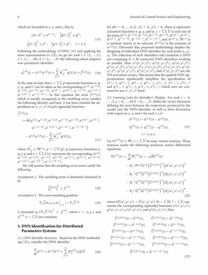
4 Journal of Control Science and Engineering
which are bounded in x, y, and z, that is,
‖σ(·)‖2 ≤ σ (l−1)+,∥∥∥ϕl(·)∥∥∥2 ≤ ϕl+,∥∥∥γl(·)∥∥∥2 ≤ γl+,
∥∥∥ψl(·)∥∥∥ ≤ ψl+, l = 1, 3.
(15)
Following the methodology of DNN [11] and applying thesame representation to (12), we get for each i ∈ (1, . . . ,L),j ∈ (1, . . . ,M), k ∈ (1, . . . ,N) the following robust adaptivenon-parametric identifier:
ui, j,kt (t) = Ai, j,kui, j,k(t) +
11∑p=1
◦W
i, j,k
p φsU(t) + f i, j,k(t). (16)
In the sum we have that s = 1, 3, φ represents functions σ , ϕ,γ, ψ, and U can be taken as the corresponding ui, j,k, ui−1, j,k,ui−2, j,k, ui, j−1,k, ui, j−2,k, ui, j,k−1, ui, j,k−2, ui−1, j−1,k, ui, j−1,k−1,ui−1, j,k−1, ui−1, j−1,k−1. In this equation the term f i, j,k(t),which is usually recognized as the modeling error, satisfiesthe following identify, and here, it has been omitted the de-pendence to xi, y j , zk of each sigmoidal function:
f i, j,k(t)
:= Φ(ui, j,k,ui−1, j,k,ui−2, j,k,ui, j−1,k,ui, j−2,k,ui, j,k−1,ui, j,k−2,
ui−1, j−1,k,ui−1, j,k−1,ui, j−1,k−1,ui−1, j−1,k−1)
− Ai, j,kui, j,k(t)−11∑p=1
◦W
i, j,k
p φsU(t),(17)
where◦W
i
p ∈ Rn×sp , p = 1, 11,φs, φ represents functions σ ,
ϕ, γ,ψ and s = 1, 3,U(t) represents the corresponding (ui, j,k,ui−1, j,k, ui−2, j,k, ui, j−1,k, ui, j−2,k, ui, j,k−1, ui, j,k−2, ui−1, j−1,k,ui−1, j,k−1, ui, j−1,k−1, ui−1, j−1,k−1).
We will assume that the modeling error terms satisfy thefollowing.
Assumption 2. The modeling error is absolutely bounded inΩ: ∥∥∥ f i, j,k∥∥∥2 ≤ f
i, j,k1 . (18)
Assumption 3. The error modeling gradient
∇s f(x, y, z, t
)∣∣∣s=si
:= ∇s fi, j,k (19)
is bounded as ‖∇s f i, j,k‖2 ≤ f
i, j,kr , where s = x, y, z and
fi, j,kr (r = 1, 3) are constants.
3. DNN Identification for DistributedParameters Systems
3.1. DNN Identifier Structure. Based on the DNN methodol-ogy [11], consider the DNN identifier
d
dtui, j,k = Ai, j,kui, j,k +
11∑p=1
Wi, j,kp (t)φsU (20)
for all i = 0, . . . ,L; u−1(t) = u−2(t) = 0, where φ representsactivation functions σ , ϕ, γ, and ψ, s = 1, 3, U is each one ofthe states ui, j,k, ui−1, j,k, ui−2, j,k, ui, j−1,k, ui, j−2,k, ui, j,k−1, ui, j,k−1,ui, j,k−2, ui−1, j−1,k, ui−1, j,k−1, ui−1, j−1,k−1, and Ai, j,k ∈ Rn×n isa constant matrix to be selected, ui, j,k(t) is the estimate ofui, j,k(t). Obviously that proposed methodology implies thedesigning of individual DNN identifier for each point xi, yj ,zk. The collection of such identifiers will constitute a DNNnet containing N × M connected DNN identifiers workingin parallel. Here σ1(xi, y j , zk), ϕ1(xi, y j , zk), ϕ2(xi, y j , zk),ϕ3(xi, y j , zk), γ1(xi, y j , zk), γ2(xi, y j , zk), γ3(xi, y j , zk), ψ1(xi,y j , zk), ψ2(xi, y j , zk), ψ3(xi, y j , zk), and σ2(xi, y j , zk) are theNN activation vectors. This means that the applied DNN-ap-proximation significantly simplifies the specification ofσ1(·, ·), ϕ1(·, ·), ϕ2(·, ·), ϕ3(·, ·), γ1(·, ·), γ2(·, ·), γ3(·, ·)and ψ1(·, ·), ψ2(·, ·), ψ3(·, ·), σ2(·, ·) which now are con-stant for any xi, y j , zk fixed.
3.2. Learning Laws for Identifier’s Weights. For each i = 0,. . . ,L, j = 0, . . . ,M, k = 0, . . . ,N , define the vector-functionsdefining the error between the trajectories produced by themodel and the DNN-identifier as well as their derivativeswith respect to x, y, and z for each i, j, k:
ui, j,k(t) := ui, j,k(t)− ui, j,k(t),
ui, j,ks (t) := u
i, j,ks (t)− ui, j,ks (t),
s = x, y, z.
(21)
Let Wi, j,kr (t) ∈ Rn, r = 1, 11 be time-variant matrices. These
matrices satisfy the following nonlinear matrix differentialequations:
Wi, j,kr (t) := d
dtW
i, j,kr (t) = −αW i, j,k
r (t)
− K−1r Pi, j,kui, j,k
(U (i, j,k),r
)ᵀ(Ωr(xi, y j , z j)
)ᵀ
− K−1r S
i, j,k1 u
i, j,kx
(U (i, j,k),r
)ᵀ(Ωrx(xi, y j , z j)
)ᵀ
− K−1r S
i, j,k2 u
i, j,ky
(U (i, j,k),r
)ᵀ(Ωry(x
i, y j , z j))ᵀ
− K−1r S
i, j,k3 u
i, j,kz
(U (i, j,k),r
)ᵀ(Ωrz(x
i, y j , z j))ᵀ
,
(22)
where Ωh(xi, y j , z j) = Sl(xi, y j , z j) (h = 1, 10, l = 1, 3) rep-resents the corresponding sigmoidal functions σ l(xi, y j , z j),ϕl(xi, y j , z j), γl(xi, y j , z j), and ψl(xi, y j , z j). Here
U (i, j,k),1(t) = ui, j,k(t), U (i, j,k),2(t) = ui−1, j,k(t),
U (i, j,k),3(t) = ui−2, j,k(t), U (i, j,k),4(t) = ui, j−1,k(t),
U (i, j,k),5(t) = ui, j−2,k(t), U (i, j,k),6(t) = ui−1, j−1,k(t),
U (i, j,k),7(t) = ui−1, j−1,k(t), U (i, j,k),8(t) = ui−1, j−1,k(t),
U (i, j,k),9(t) = ui−1, j−1,k(t), U (i, j,k),10(t) = ui−1, j−1,k(t),
U (i, j,k),11(t) = ui−1, j−1,k−1(t)(23)

Journal of Control Science and Engineering 5
with positive matrices Kr(r = 1, 11) and Pi, j,k, Si, j,k1 , and S
i, j,k2
(i = 0,N ; j = 0,M) which are positive definite solutions
(Pi, j > 0, Si, j1 > 0, S
i, j2 > 0) and S
i, j,k3 (i = 0,N ; j = 0,M, k =
0,L) of the algebraic Riccati equations defined as follows:
Ric(Pi, j,k
):= Pi, j,kAi, j,k +
[Ai, j,k
]ᵀPi, j,k
+ Pi, j,kRi, j,kP Pi, j,k +Q
i, j,kP = 0,
Ric(Si, j,k1
):= S
i, j,k1 Ai, j,k +
[Ai, j
]ᵀSi, j,k1
+ Si, j,k1 R
i, j,kS1
Si, j,k1 +Q
i, j,kS1
= 0,
Ric(Si, j,k2
):= S
i, j,k2 Ai, j,k +
[Ai, j,k
]ᵀSi, j,k2
+ Si, j,k2 R
i, j,kS2
Si, j,k2 +Q
i, j,kS2
= 0,
Ric(Si, j,k3
):= S
i, j,k3 Ai, j,k +
[Ai, j,k
]ᵀSi, j,k3
+ Si, j,k3 R
i, j,kS3
Si, j,k3 +Q
i, j,kS3
= 0,
(24)
where each Ri, j,kB has the form
Ri, j,kB :=
11∑r=1
◦W
i, j,k
r Λr+b
(◦W
i, j,k
r
)ᵀ+ Λb, (25)
where B can be P, S1, S2, and S3 and b = (7, 14, 21, 28).
Matrices Qi, j,kB have the form
Qi, j,kB :=
∥∥∥Ω1m(xi, y j , zk)
∥∥∥2
Λ−11
+∥∥∥Ω2
m(xi−1, y j , zk)∥∥∥2
Λ−12
+∥∥∥Ω3
m(xi−2, y j , zk)∥∥∥2
Λ−13
+∥∥∥Ω4
m(xi, y j−1, zk)∥∥∥2
Λ−14
+∥∥∥Ω5
m(xi, y j−2, zk)∥∥∥2
Λ−15
+∥∥∥Ω6
m(xi, y j , zk−1)∥∥∥2
Λ−16
+∥∥∥Ω7
m(xi, y j , zk−2)∥∥∥2
Λ−17
+∥∥∥Ω8
m(xi−1, y j−1, zk)∥∥∥2
Λ−18
+∥∥∥Ω9
m(xi, y j−1, zk−1)∥∥∥2
Λ−19
+∥∥∥Ω10
m (xi−1, y j , zk−1)∥∥∥2
Λ−110
+∥∥∥Ω11
m (xi−1, y j−1, zk−1)∥∥∥2
Λ−111
+Qi, j,kB ,
(26)
where B can be P, S1, S2, or S3, representing the partial deri-vative; for S1 it is with respect to x, for S2 with respect to y,and for S3 with respect to z, and Λ−1
l (l = 1, 46), where
Ωrx
(xi, yj , zj
):= d
dxΩr(x, y, z
)∣∣∣∣x=xi,y=yj ,z=zk
,
Ωry
(xi, yj , zj
):= d
dyΩr(x, y, z
)∣∣∣∣∣x=xi,y=yj ,z=zk
,
Ωrz
(xi, yj , zj
):= d
dzΩr(x, y, z
)∣∣∣∣x=xi,y=yj ,z=zk
.
(27)
Here, Wi, j,kk (t) :=W
i, j,kk (t)−
◦W
i, j,k
k , k = 1, 11.The special class of Riccati equation
PA + ATP + PRP +Q = 0 (28)
has a unique positive solution P if and only if the four con-ditions given in [11] (page 65, chapter 2 Nonlinear SystemIdentification: Differential Learning) are fulfilled (see [11]):(1) matrix A is stable, (2) pair (A,R1/2) is controllable, (3)pair (Q1/2,A) is observable, and (4) matrices (A,Q,R) shouldbe selected in such a way to satisfy the following inequality:
14
(AᵀR−1 − R−1A
)R(AᵀR−1 − R−1A
)ᵀ+Q ≤ AᵀR−1A
(29)
which restricts the largest eigenvalue of R guarantying theexistence of a unique positive solution. The main result ob-tained in this part is in the practical stability framework.
4. Practical Stability and Stabilization
The following definition and proposition are needed for themain results of the paper. Consider the following ODE non-linear system:
zt = g(zt, vt) + �t (30)
with zt ∈ Rn, and vt ∈ Rm, and �t an external perturbationor uncertainty such that ‖�t‖2 ≤ �+.
Definition 4 (Practical Stability). Assume that a time intervalT and a fixed function v∗t ∈ Rm over T are given. Givenε > 0, the nonlinear system (30) is said to be ε-practicallystable over T under the presence of �t if there exists a δ > 0(δ depends on ε and the interval T) such that zt ∈ B[0, ε], forall 0 ≤ t, whenever zt0 ∈ B[0, δ].
Similarly to the Lyapunov stability theory for nonlinearsystems, it was applied the aforementioned direct method forthe ε-practical stability of nonlinear systems using-practicalLyapunov-like functions under the presence of external per-turbations and model uncertainties. Note that these func-tions have properties differing significantly from the usualLyapunov functions in classic stability theory.
The subsequent proposition requires the following lem-ma.
Lemma 5. Let a nonnegative function V(t) satisfying the fol-lowing differential inequality:
V(t) ≤ −αV(t) + β, (31)
where α > 0 and β ≥ 0. Then[1− μ√
V(t)
]+
−→ 0, (32)
with μ =√β/α and the function [·]+ defined as
[z]+ :=⎧⎨⎩z if z ≥ 0,
0 if z < 0.(33)

6 Journal of Control Science and Engineering
Proof. The proof of this lemma can be obtained directly bythe application of the Gronwall-Bellman Lemma.
Proposition 6. Given a time interval T and a function v(·)over a continuously differentiable real-valued function V(z, t)satisfying V(0, t) = 0, for all tεT , is said to be ε-practical Lya-punov-like function over T under v if there exists a constantα > 0 such that
V(z, t) ≤ −αV(z, t) +H(�+), (34)
with H a bounded nonnegative nonlinear function with upperbound H+. Moreover, the trajectories of zt belong to the zoneε := H+/α when t → ∞. In this proposition V(zt, t) denotesthe derivative of V(z, t) along zt, that is, V(z, t) = Vz(z, t) ·(g(zt, vt) + �t) +Vt(x, t).
Proof. The proof follows directly from Lemma 5.
Definition 7. Given a time interval T and a function v(·) overT , nonlinear system (30) is ε-practically stable, T under vif there exists an ε-practical Lyapunov-like function V(x, t)over T under v.
5. Identification Problem Formulation
The state identification problem for nonlinear systems (13)analyzed in this study, could be now stated as follows.
Problem. For the nonlinear system, given by the vector PDE(20), to study the quality of the DNN identifier supplied withthe adjustment (learning) laws (22), estimate the upperbound of the identification error δ given by
δ := limt→∞
L∑i=0
M∑j=0
N∑k=0
∥∥∥ui, j,k(t)− ui, j,k(t)∥∥∥2
Pi, j,k(35)
(with Pi, j,k from (24)) and, if it is possible, to reduce to itslowest possible value, selecting free parameters participatinginto the DNN identifier (A,Kr , r = 1, 11).
This implicates that the reduction of the identificationerror δ means that the differential neural network has con-verged to the solution of the 3D PDE; this can be observed inthe matching of the DNN to the PDE state.
6. Main Result
The main result of this paper is presented in the followingtheorem.
Theorem 8. Consider the nonlinear model (1) (i = 0, . . . ,L;j = 0, . . . ,M, k = 0, . . . ,N), given by the system of PDEs withuncertainties (perturbations) in the states, under the borderconditions (2). Let us also suppose that the DNN-identifier isgiven by (20) which parameters are adjusted by the learning
laws (22) with parameters αi, j,km (i = 0, . . . ,L; j = 0, . . . ,M; k =
0, . . . ,N). If positive definite matrices Qi, j,k1 , Q
i, j,k2 , and Q
i, j,k3
provide the existence of positive solutions Pi, j , Si, j,k1 , S
i, j,k2 , and
02
46
8
02
46
8
Solution of 3D partial differential equation at time
10
10
10
Coordinate yt
0
10
20
30
40
50
60
Coordinate xt
u(x
,y,z
,t)
Figure 2: Numerical trajectory produced by the mathematicalmodel described by 3D partial differential equation at time 10 salong the whole domain.
02
46
8
02
46
8 10
10
Coordinate yt
0
10
20
30
40
50
60
Coordinate xt
ue(x,y,z,t)
Approximation of 3D differential neural network at time 10
Figure 3: Numerical trajectory produced by the neural network de-scribed reproducing the model at time 10 s along the whole domain.
Difference between 3D PDE and 3D DNN at time 10
−0.8−0.6−0.4
−0.20
0.20.4
0.60.8
02
46
8
02
46
8 10
10
Coordinate yt Coordinate xt
−u
(x,y
,z,t
)ue(x,y,z,t)
Figure 4: Error of the approximation. Difference between 3D PDEnumerical solution and 3D DNN approximation at time 10 s alongthe whole domain.

Journal of Control Science and Engineering 7
Si, j,k3 (i = 0, . . . ,L) to the Riccati equations (24), then for alli = 0, . . . ,L; j = 0, . . . ,M; k = 0, . . . ,N the following ρ-upperbound:
limt→∞
L∑i=0
M∑j=0
×N∑k=0
[∥∥∥ui, j,k(t)− ui, j,k(t)∥∥∥2
Pi, j,k+∥∥∥ui, j,kx (t)− ui, j,kx (t)
∥∥∥Si, j,k1
+∥∥∥ui, j,ky (t)− ui, j,ky (t)
∥∥∥Si, j,k2
+∥∥∥ui, j,kz (t)− ui, j,kz (t)
∥∥∥Si, j,k3
]≤ μ
(36)
is ensured with μ0 := √LMNα−1/2 and
μ := μ0
√maxi, j,k
Ψ,
Ψ := �3∑s=1
fi, j,ks
≥(f i, j,k(t)
)TΛ−1
7 f i, j,k(t) +(fi, j,kx (t)
)TΛ−1
14 fi, j,kx (t)
+(fi, j,ky (t)
)TΛ−1
21 fi, j,ky (t) +
(fi, j,kz (t)
)TΛ−1
28 fi, j,kz (t),
� := max{λmax
(Λ−1
7
), λmax
(Λ−1
14
), λmax
(Λ−1
21
), λmax
(Λ−1
28
)}.
(37)
Moreover, the weights Wr,tr = 1, 11 remain bounded beingproportional to μ, that is, ‖Wr,t‖ ≤ Krμ, r = 1, 11.
Proof. The proof is given in the appendix.
7. Simulation Results
7.1. Numerical Example. Below, the numerical smulationshows the qualitative illustration for a benchmark system.Therefore, consider the following three-dimensional PDEdescribed as follows:
ut(x, y, z, t
) = −c1uxx(x, y, z, t
)− c2uyy(x, y, z, t
)− c3uzz
(x, y, z, t
)+ ξ(x, y, z, t
),
(38)
where c1 = c2 = c3 = 0.15. It is assumed that there is accessto discrete measurements of the state u(x, y, z, t) along thewhole domain, which is feasible in practice. ξ(x, y, z, t) is anoise in the state dynamics. This model will be used just togenerate the data to test the 3D identifier based on DNN.Boundary conditions and initial conditions were selected asfollows:
u(0, 0, 0, t) = rand(1), ux(0, 0, 0, t) = 0,
uy(0, 0, 0, t) = 0, uz(0, 0, 0, t) = 0.(39)
The trajectories of the model can be seen in Figure 3 as wellas the estimated state, produced by the DNN identifier. The
2 3 4 5
5
6 7 8 9
Coordinate zt
3D PDE solution and 3D DNN approximation at time 10
3D PDE solution3D DNN approximation
0
1
1
0
10
15
20
25
30
35
40
45
50
u(x
,y,z
,t)
andue(x,y,z,t)
Figure 5: Comparison between 3D PDE trajectories and 3D DNNapproximation for coordinate z at time 10 s.
0 50 100 150 2000
50
100
150
200
250
300
350
400Index error
t
||ue(x,y,t)−u
(x,y
,t)||
2
Figure 6: Index quadratic error for the whole time with coordinatesx, y, and z fixed.
efficiency of the identification process provided by the sug-gested DNN algorithm shown in Figure 4.
In Figures 5 and 6 there are shown the trajectories of thePDE and the DNN for the coordinate z and the index errorof the PDE and the DNN at 10 seconds for coordinates x, z,respectively Figure 2.
7.2. Tumour Growth Example. The mathematical model ofthe brain tumour growth is presented in this section based onthe results of [18]. Here the diffusion coefficient is consideredas a constant. Let consider the following three-dimensional
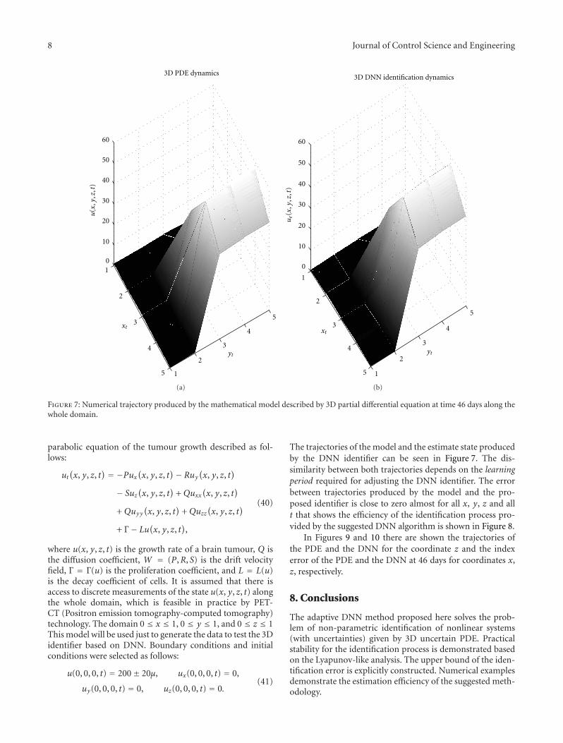
8 Journal of Control Science and Engineering
3D PDE dynamics
xt
yt4
4
5
5
1
1
2
2
3
3
0
10
20
30
40
50
60
u(x
,y,z
,t)
(a)
xt
yt4
4
5
5
1
1
2
2
3
3
0
10
20
30
40
50
60
3D DNN identification dynamics
ue(x,y,z,t)
(b)
Figure 7: Numerical trajectory produced by the mathematical model described by 3D partial differential equation at time 46 days along thewhole domain.
parabolic equation of the tumour growth described as fol-lows:
ut(x, y, z, t
) = −Pux(x, y, z, t)− Ruy(x, y, z, t
)− Suz
(x, y, z, t
)+Quxx
(x, y, z, t
)+Quyy
(x, y, z, t
)+Quzz
(x, y, z, t
)+ Γ− Lu(x, y, z, t
),
(40)
where u(x, y, z, t) is the growth rate of a brain tumour, Q isthe diffusion coefficient, W = (P,R, S) is the drift velocityfield, Γ = Γ(u) is the proliferation coefficient, and L = L(u)is the decay coefficient of cells. It is assumed that there isaccess to discrete measurements of the state u(x, y, z, t) alongthe whole domain, which is feasible in practice by PET-CT (Positron emission tomography-computed tomography)technology. The domain 0 ≤ x ≤ 1, 0 ≤ y ≤ 1, and 0 ≤ z ≤ 1This model will be used just to generate the data to test the 3Didentifier based on DNN. Boundary conditions and initialconditions were selected as follows:
u(0, 0, 0, t) = 200± 20μ, ux(0, 0, 0, t) = 0,
uy(0, 0, 0, t) = 0, uz(0, 0, 0, t) = 0.(41)
The trajectories of the model and the estimate state producedby the DNN identifier can be seen in Figure 7. The dis-similarity between both trajectories depends on the learningperiod required for adjusting the DNN identifier. The errorbetween trajectories produced by the model and the pro-posed identifier is close to zero almost for all x, y, z and allt that shows the efficiency of the identification process pro-vided by the suggested DNN algorithm is shown in Figure 8.
In Figures 9 and 10 there are shown the trajectories ofthe PDE and the DNN for the coordinate z and the indexerror of the PDE and the DNN at 46 days for coordinates x,z, respectively.
8. Conclusions
The adaptive DNN method proposed here solves the prob-lem of non-parametric identification of nonlinear systems(with uncertainties) given by 3D uncertain PDE. Practicalstability for the identification process is demonstrated basedon the Lyapunov-like analysis. The upper bound of the iden-tification error is explicitly constructed. Numerical examplesdemonstrate the estimation efficiency of the suggested meth-odology.

Journal of Control Science and Engineering 9
0
2
4
6
1
2
3
4
5−1
−0.5
0
0.5
1
Error dynamics
−u
(x,y
,z,t
)ue(x,y,z,t)
xtyt
Figure 8: Error of the approximation. Difference between 3D PDEnumerical solution and 3D DNN approximation at time 46 daysalong the whole domain.
21 3 4 5 6 7 8 9 10
10
20
30
40
50
60
Coordinate zt
u(x
,y,z
,t)
&ue(x,y,z,t)
3D PDE solution3D DNN approximation
0
Figure 9: Comparison between 3D PDE trajectories and 3D DNNapproximation for coordinate z at time 46 days.
Appendix
Consider the Lyapunov-like function defined as the compo-sition of NML individual Lyapunov functions V i, j,k(t) alongthe whole space:
V(t) :=L∑i=0
M∑j=0
N∑k=0
⎡⎣V i, j,k(t) +
11∑r=1
tr{[W i
r(t)]TKrW
ir(t)
}⎤⎦,
Vi, j,k
(t) :=∥∥∥ui, j,k(t)
∥∥∥2
Pi, j,k+∥∥∥ui, j,kx (t)
∥∥∥2
Si, j,k1
+∥∥∥ui, j,ky (t)
∥∥∥2
Si, j,k2
+∥∥∥ui, j,kz (t)
∥∥∥2
Si, j,k3.
(A.1)
20 40 60 80 100 120 140 160 180 20000
50
100
150Index error
t
||ue(x,y,t)−u
(x,y
,t)||
2
Figure 10: Index quadratic error for the whole time with coordi-nates x, y, and z fixed.
The time derivative V(t) of V(t) can be obtained so that
V(t) = 2N∑i=0
M∑j=0
L∑k=0
(ui, j,k(t)
)T(t)Pi· j,k
d
dtui, j,k(t)
+ 2N∑i=0
M∑j=0
L∑k=0
[ui, j,kx (t)
]TSi· j,k1
d
dtui. j,kx (t)
+ 2N∑i=0
M∑j=0
L∑k=0
[ui, j,ky (t)
]TSi· j,k2
d
dtui. j,ky (t)
+ 2N∑i=0
M∑j=0
L∑k=0
[ui, j,kz (t)
]TSi· j,k3
d
dtui. j,kz (t)
+ 2N∑i=0
M∑j=0
L∑k=0
3∑r=1
tr{[W
i, j,kr (t)
]TKrW
i, j,kr (t)
}.
(A.2)
Applying the matrix inequality given in [19]
XYT + YXT ≤ XΛXT + YΛ−1YT (A.3)
valid for any X ,Y ∈ Rr×s and for any 0 < Λ = ΛT ∈ Rs×s
to the terms containing f i(t) and their derivatives. We obtain
V(t) ≤ I1(t) + I2(t) + I3(t) + I4(t)
− 2α11∑r=1
N∑i=0
M∑j=0
L∑k=0
tr{(W
i, jr (t)
)TKrW
i, j,kr (t)
}
+ 2α11∑r=1
N∑i=0
M∑j=0
L∑k=0
tr{(W
i, jr (t)
)TKrW
i, j,kr (t)
}
+ 211∑r=1
N∑i=0
M∑j=0
L∑k=0
tr{(W
i, jr (t)
)TK2r W
i, j,k1 (t)
}
−N∑i=0
M∑j=0
L∑k=0
αVi, j,k
(t) + �N∑i=0
M∑j=0
L∑k=0
3∑s=1
fi, j,ks ,
(A.4)

10 Journal of Control Science and Engineering
where
I1(t) :=N∑i=0
M∑j=0
L∑k=0
(ui. j,k(t)
)TRic(Pi, j)ui, j,k(t),
I2(t) :=N∑i=0
M∑j=0
L∑k=0
(ui. j,kx (t)
)TRic(Si, j,k1
)ui, j,kx (t),
I3(t) :=N∑i=0
M∑j=0
L∑k=0
(ui. j,ky (t)
)TRic(Si, j2
)ui, j,ky (t),
I4(t) :=N∑i=0
M∑j=0
L∑k=0
(ui. j,kz (t)
)TRic(Si, j3
)ui, j,kz (t).
(A.5)
By the Riccati equations, defined in (24), I1(t) = I2(t) =I3(t) = I4(t) = 0, and in view of the adjust equations of theweights (22), the previous inequality is simplified to
V(t) ≤ −αN∑i=0
M∑j=0
L∑k=0
Vi, j,k
(t)
+ 2α11∑r=1
N∑i=0
M∑j=0
L∑k=0
tr{(W
i, jr (t)
)TKrW
i, j,kr (t)
}
+ ΨV(t) ≤ −αN∑i=0
M∑j=0
L∑k=0
V i, j,k(t) + Ψ.
(A.6)
Applying Lemma 5, one has [1− (μ/√V(t))]+ → 0,
which completes the proof.
References
[1] Y. Pinchover and J. Rubinstein, An Introduction to PartialDifferential Equations, Cambridge University Press, 2008.
[2] G. D. Smith, Numerical Solution of Partial Differential Equa-tions: Infinite Difference Methods, Clarendon Press, Oxford,UK, 1978.
[3] T. J. R. Hughes, The Finite Element Method, Prentice Hall, Up-per Saddle River, NJ, USA, 1987.
[4] R. Fuentes, A. Poznyak, T. Poznyak, and I. Chairez, “Neuralnumerical modeling for uncertain distributed parameter sys-tem,” in Proceedings of the International Joint Conference inNeural Networks, pp. 909–916, Atlanta, Ga, USA, June 2009.
[5] S. Haykin, Neural Networks. A Comprehensive Foundation,IEEE Press, Prentice Hall U.S., New York, NY, USA, 2nd edi-tion, 1999.
[6] G. Cybenko, “Approximation by superposition of sigmoidalactivation function,” Mathematics of Control, Signals and Sys-tems, vol. 2, pp. 303–314, 1989.
[7] I. E. Lagaris, A. Likas, and D. I. Fotiadis, “Artificial neural net-works for solving ordinary and partial differential equations,”IEEE Transactions on Neural Networks, vol. 9, no. 5, pp. 987–1000, 1998.
[8] M. W.M Dissanayake and N. Phan-Thien, “Neural-network-based approximations for solving partial differential equa-tions,” Communications in Numerical Methods in Engineering,vol. 10, no. 3, pp. 195–201, 1994.
[9] N. Mai-Duy and T. Tran-Cong, “Numerical solution ofdifferential equations using multiquadric radial basis functionnetworks,” Neural Networks, vol. 14, no. 2, pp. 185–199, 2001.
[10] S. He, K. Reif, and R. Unbehauen, “Multilayer neural networksfor solving a class of partial differential equations,” Neural Net-works, vol. 13, no. 3, pp. 385–396, 2000.
[11] A. Poznyak, E. Sanchez, and W. Yu, Differential Neural Net-works for Robust Nonlinear Control (Identification, Estate Esti-mation an trajectory Tracking), World Scientific, 2001.
[12] F. L. Lewis, A. Yesildirek, and K. Liu, “Multilayer neural-netrobot controller with guaranteed tracking performance,” IEEETransactions on Neural Networks, vol. 7, no. 2, pp. 1–11, 1996.
[13] G. A. Rovithakis and M. A. Christodoulou, “Adaptive controlof unknown plants using dynamical neural networks,” IEEETransactions on Systems, Man and Cybernetics, vol. 24, no. 3,pp. 400–412, 1994.
[14] H. K. Khalil, Nonlinear Systems, Prentice-Hall, Upper SaddleRiver, NJ, USA, 2002.
[15] R. A. Adams and J. Fournier, Sobolev Spaces, Academic Press,New York, NY, USA, 2nd edition, 2003.
[16] B. Delyon, A. Juditsky, and A. Benveniste, “Accuracy analysisfor wavelet approximations,” IEEE Transactions on Neural Net-works, vol. 6, no. 2, pp. 332–348, 1995.
[17] N. E. Cotter, “The Stone-Weierstrass theorem and its appli-cation to neural networks,” IEEE Transactions on Neural Net-works, vol. 1, no. 4, pp. 290–295, 1990.
[18] M. R. Islam and N. Alias, “A case study: 2D Vs 3D partial dif-ferential equation toward tumour cell visualisation on multi-core parallel computing atmosphere,” International Journal forthe Advancement of Science and Arts, vol. 10, no. 1, pp. 25–35,2010.
[19] A. Poznyak, Advanced Mathetical Tools for Automatic ControlEngineers, Deterministic Technique, vol. 1, Elsevier, 2008.


