
Optimization


Transportation Planning


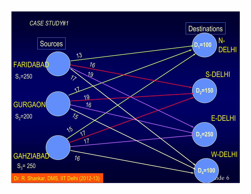
Example#1: Transportation, Problems

�Can be formulated as linear programs and solved by general purpose linear programming codes.

� However, there are many computer packages, which contain separate computer codes for these models which take advantage of their network structure.


Transportation Problem

�The transportation problem seeks to minimize the total shipping costs of transporting goods from m origins (each with a supply si ) to n destinations (each with a demand dj ), when the unit shipping cost from an origin, i, to a destination, j, is cij.


N-DELHI

S-DELHI

E-DELHI

W-DELHI

Destinations

Sources

FARIDABAD

GURGAON

GAHZIABAD

S1=250

S2=200

S3= 250

D1=100

D2=150

D3=250

D4=100

17

19

16

17

13

19

16

15

1517

17

16

CASE STUDY#1


TP: a Linear Programming Model

•The structure of the model is:

� Minimize Total Shipping Cost� ST

� [Amount shipped from a source] <= [Supply at that source]

� [Amount received at a destination]=[Demand at that Destination]

• Decision variables� Xij = the number of cases shipped from plant i to warehouse j.

� where: i=1 (FARIDABAD), 2 (GURGAON), 3 (GHAZIABAD)

j=1 (N-DELHI), 2 (S-DELHI), 3 (E-DELHI), 4(W-DELHI)


N-Delhi

S-Delhi

E-Delhi

W-Delhi

D1=100

D2=150

D3=250

D4=100

The supply constraints

Faridabad

S1=250

X11

X12

X13

X14

Supply from FARIDABAD X11+X12+X13+X14 = 250

Gurgaon

S2=200

X21

X22

X23

X24

Supply from GURGAON X21+X22+X23+X24 = 200

GhaziabadS3= 250

X31

X32

X33

X34

Supply from Ghaziabad X31+X32+X33+X34 = 250

CASE STUDY


The complete mathematical model

Minimize 13X11+16X12+19X13+ 17X14 +17X21+19X22+16X23+15X24+

15X31+17X32+17X33+16X34

ST

Supply constrraints:

X11+ X12+ X13+ X14 250

X21+ X22+ X23+ X24 200

X31+ X32+ X33+ X34 250

Demand constraints:

X11+ X21+ X31 100

X12+ X22+ X32 150

X13+ X23+ X33 250

X14+ X24+ X34 100

All Xij are nonnegative

≤

≤

≤

=

=

=

=

Total shipment out of a supply nodecannot exceed the supply at the node.

Total shipment received at a destinationnode, must equal the demand at that node.

CASE STUDY


The complete mathematical model

Minimize 13X11+16X12+19X13+ 17X14 +17X21+19X22+16X23+15X24+

15X31+17X32+17X33+16X34

ST

Supply constrraints:

X11+ X12+ X13+ X14 250

X21+ X22+ X23+ X24 200

X31+ X32+ X33+ X34 250

Demand constraints:

X11+ X21+ X31 100

X12+ X22+ X32 150

X13+ X23+ X33 250

X14+ X24+ X34 100

All Xij are nonnegative

≤

≤

≤

=

=

=

=

Total shipment out of a supply nodecannot exceed the supply at the node.

Total shipment received at a destinationnode, must equal the demand at that node.

CASE STUDY#6


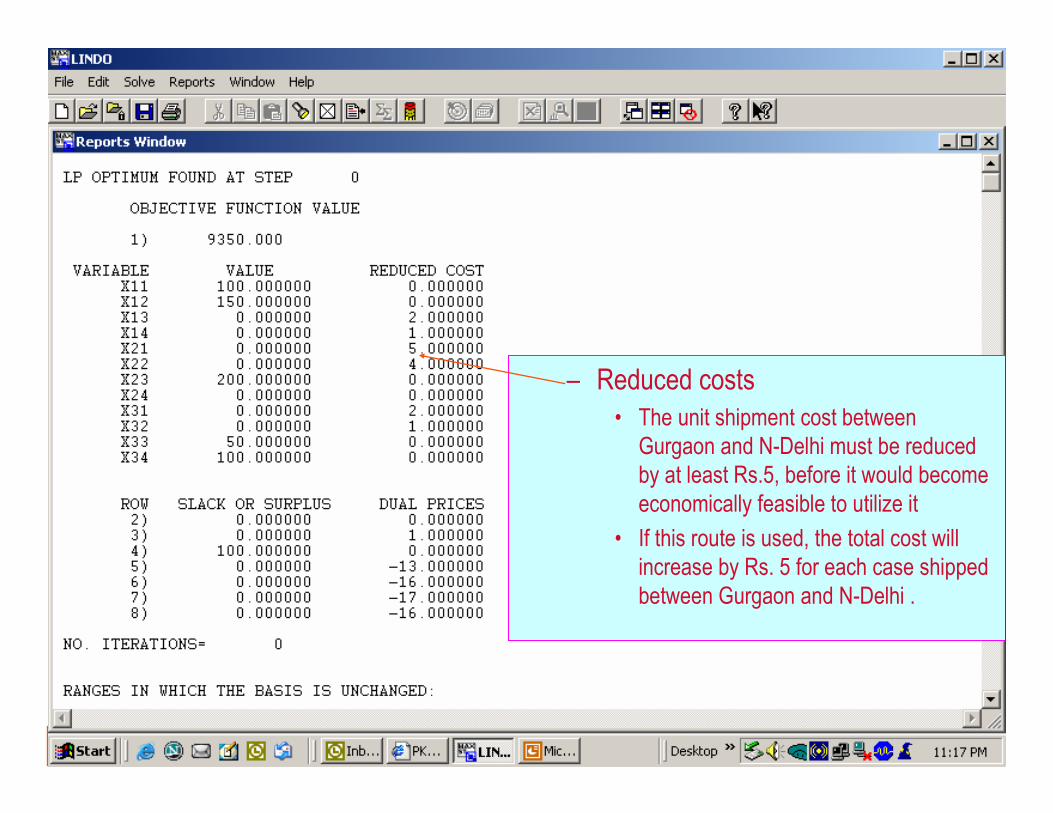
– Reduced costs • The unit shipment cost between

Gurgaon and N-Delhi must be reduced by at least Rs.5, before it would become economically feasible to utilize it

• If this route is used, the total cost will increase by Rs. 5 for each case shipped between Gurgaon and N-Delhi .


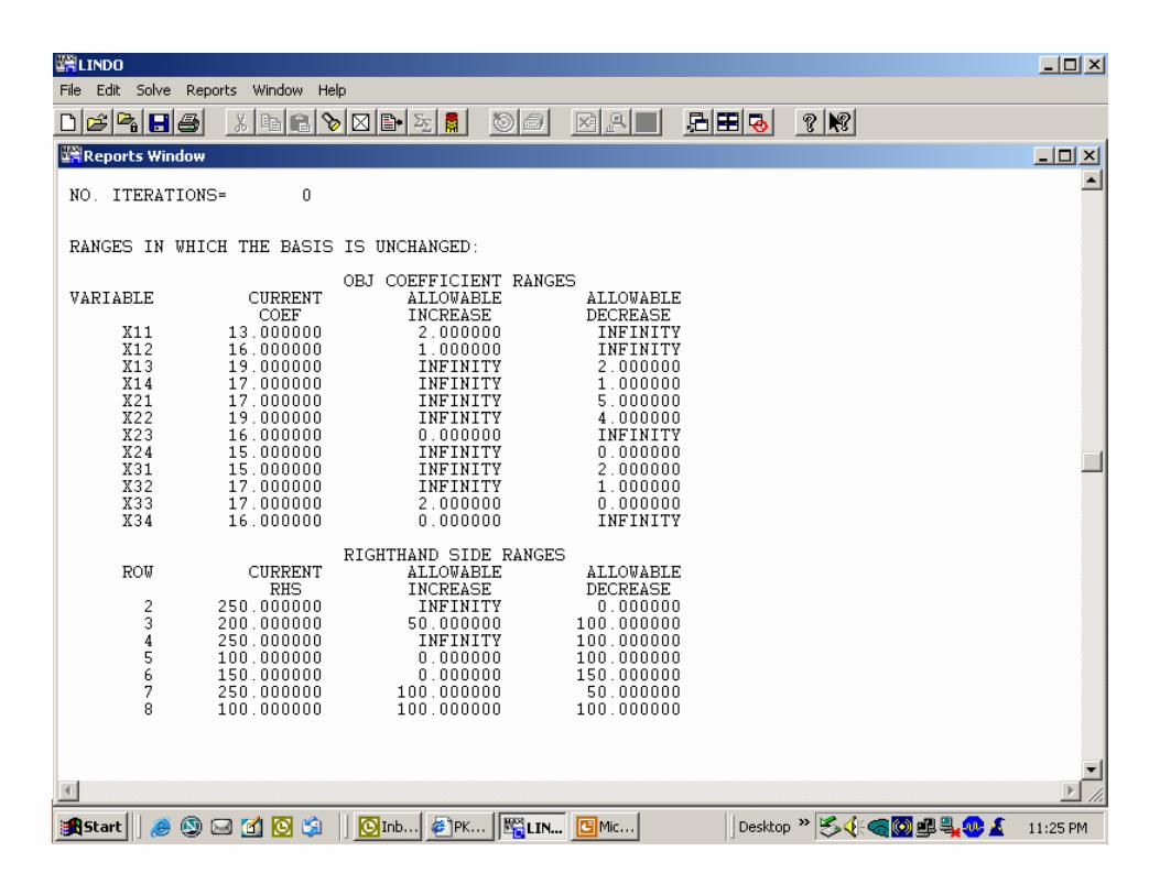
– Allowable Increase/Decrease• This is the range of optimality.

• The unit shipment cost between Gurgaon and N-Delhi may increase up to any level or decrease up to Rs. 5 with no change in the current optimal transportation plan.


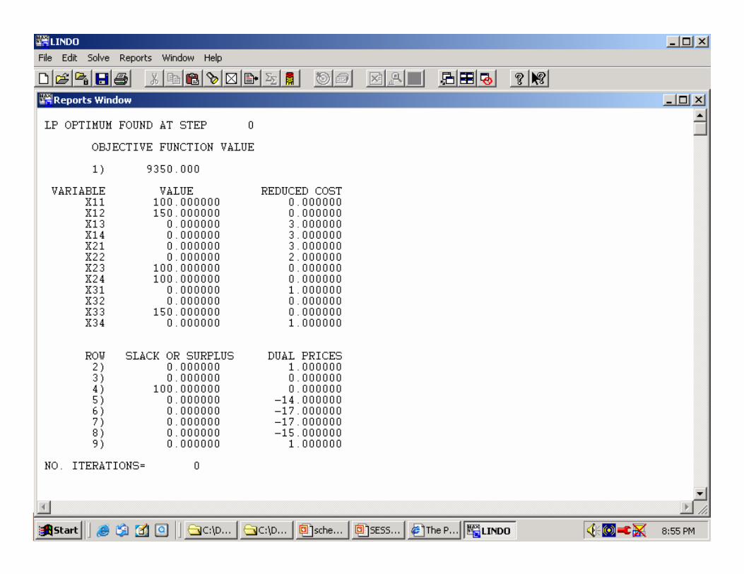
Another solution: Yet optimal


Network Planning


Solution Techniques

� Mathematical optimization techniques:

1. Exact algorithms: find optimal solutions

2. Heuristics: find “good” solutions, not necessarily optimal

� Simulation models: provide a mechanism to evaluate specified design alternatives created by the designer.


Example

� Single product

� Two plants p1 and p2

• Plant p2 has an annual capacity of 60,000 units.

� The two plants have the same production costs.

� There are two warehouses w1 and w2 with identical warehouse handling costs.

� There are three markets areas c1,c2 and c3 with demands of 50,000, 100,000 and 50,000, respectively.


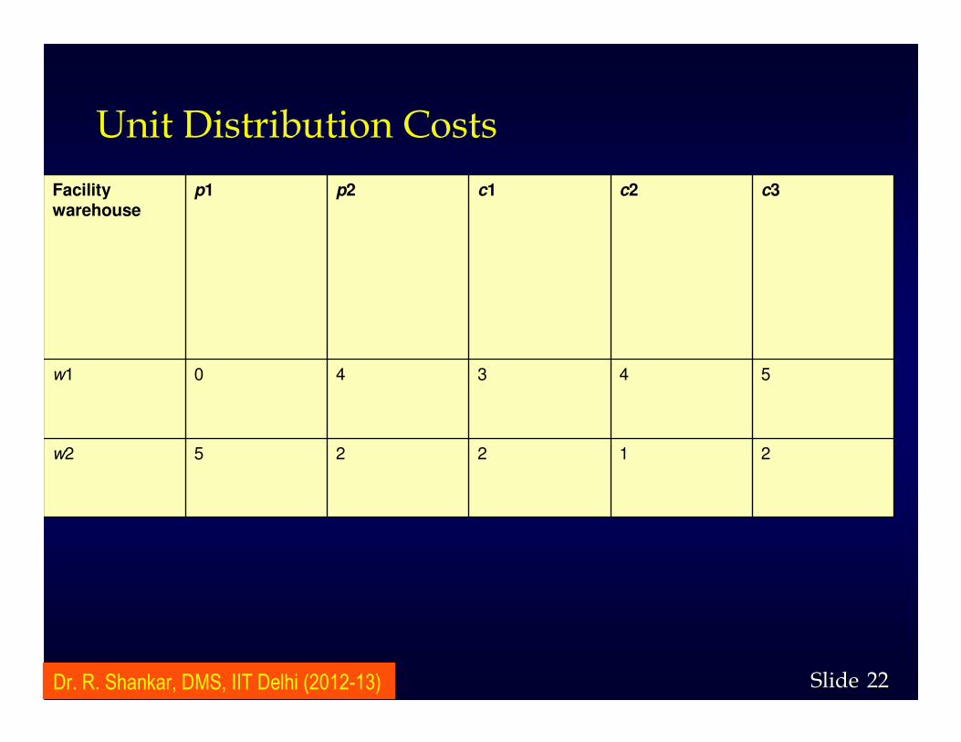
Unit Distribution Costs

Facility

warehouse

p1 p2 c1 c2 c3

w1 0 4 3 4 5

w2 5 2 2 1 2


CASE : NETWORK PROBLEM

� Network Representation

ARNOLD

WASH

BURN

ZROX

HEWES

200,000200,000

60,000060,0000

50,00050,000

100,000100,000

50,00050,000

00

55

44

22

33

44

55

22 11

22

P1P1

P2P2

C2C2

C1C1

W1W1

W2W2

C3C3


Heuristic #1:Choose the Cheapest Warehouse to Source Demand

D = 50,000

D = 100,000

D = 50,000

Cap = 60,000

$5 x 140,000

$2 x 60,000

$2 x 50,000

$1 x 100,000

$2 x 50,000

Total Costs = $1,120,000


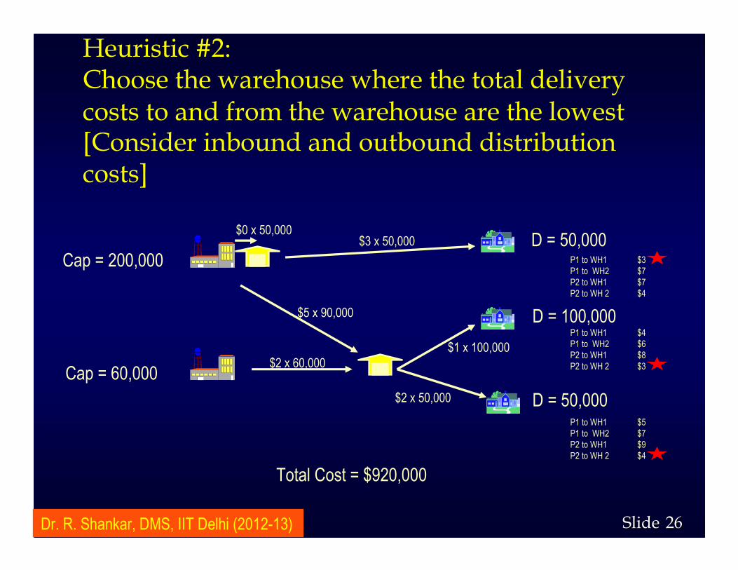
Heuristic #2:Choose the warehouse where the total delivery costs to and from the warehouse are the lowest[Consider inbound and outbound distribution costs]

D = 50,000

D = 100,000

D = 50,000

Cap = 60,000

$4

$5

$2

$3

$4$5

$2

$1

$2

$0

P1 to WH1 $3P1 to WH2 $7P2 to WH1 $7P2 to WH 2 $4



Market #1 is served by WH1, Markets 2 and 3are served by WH2


D = 50,000

D = 100,000

D = 50,000

Cap = 60,000

Cap = 200,000

$5 x 90,000

$2 x 60,000

$3 x 50,000

$1 x 100,000

$2 x 50,000

$0 x 50,000




Total Cost = $920,000

Heuristic #2:Choose the warehouse where the total delivery costs to and from the warehouse are the lowest[Consider inbound and outbound distribution costs]


The Optimization Model

The problem described earlier can be framed as the following linear programming problem.

Let

� x(p1,w1), x(p1,w2), x(p2,w1) and x(p2,w2) be the flows from the plants to the warehouses.

� x(w1,c1), x(w1,c2), x(w1,c3) be the flows from the warehouse w1 to customer zones c1, c2 and c3.

� x(w2,c1), x(w2,c2), x(w2,c3) be the flows from warehouse w2 to customer zones c1, c2 and c3


The problem we want to solve is: min 0x(p1,w1) + 5x(p1,w2) + 4x(p2,w1)

+ 2x(p2,w2) + 3x(w1,c1) + 4x(w1,c2)

+ 5x(w1,c3) + 2x(w2,c1) + 2x(w2,c3)

subject to the following constraints:x(p2,w1) + x(p2,w2) ≤ 60000

x(p1,w1) + x(p2,w1) = x(w1,c1) + x(w1,c2) + x(w1,c3)


x(w1,c1) + x(w2,c1) = 50000

x(w1,c2) + x(w2,c2) = 100000

x(w1,c3) + x(w2,c3) = 50000

all flows greater than or equal to zero.



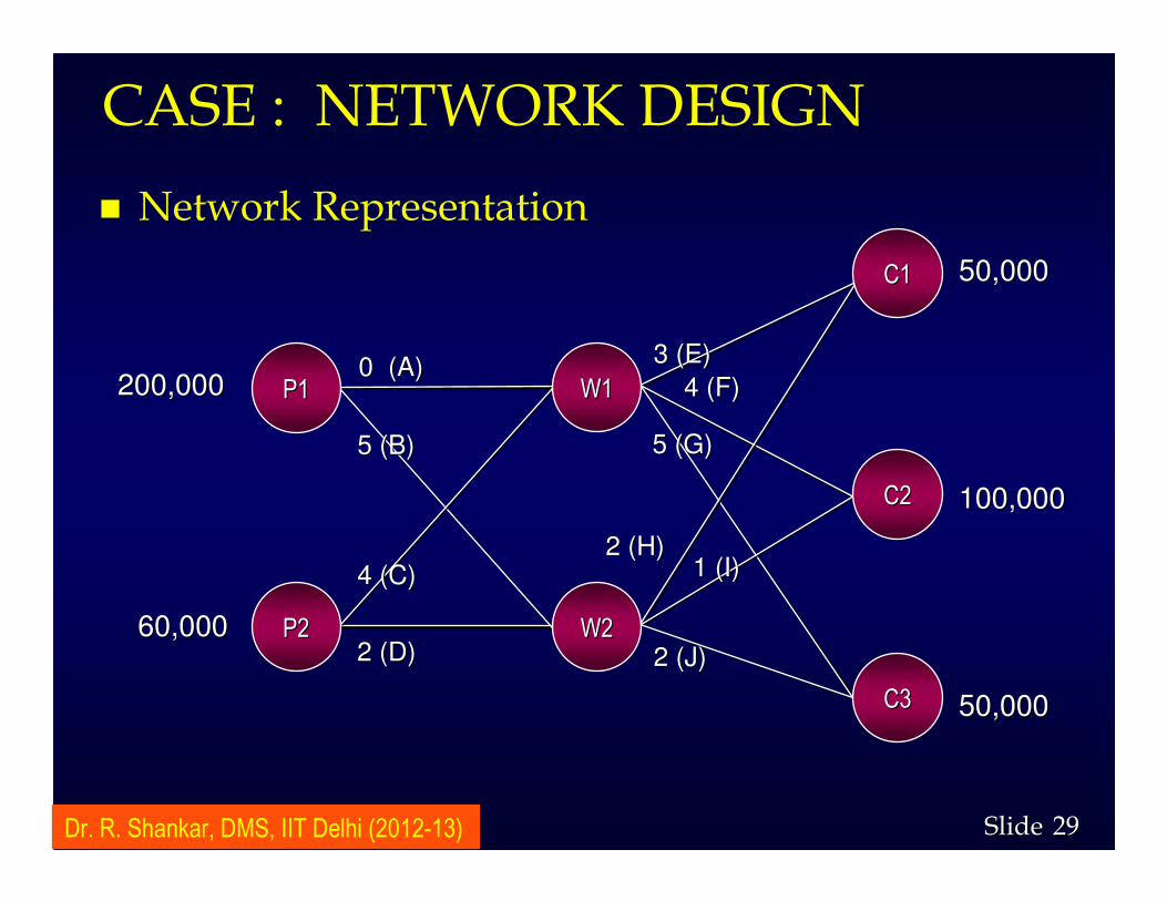
CASE : NETWORK DESIGN


ARNOLD

WASH

BURN

ZROX

HEWES

200,000200,000

60,00060,000

50,00050,000

100,000100,000

50,00050,000

0 (A)0 (A)

5 (B)5 (B)

4 (C)4 (C)

2 (D) 2 (D)

3 (E)3 (E)

4 (F)4 (F)

5 (G)5 (G)

2 (H)2 (H)1 (I)1 (I)

2 (J)2 (J)

P1P1

P2P2

C2C2

C1C1

W1W1

W2W2

C3C3


The problem we want to solve is: min 0x(p1,w1) + 5x(p1,w2) + 4x(p2,w1)

+ 2x(p2,w2) + 3x(w1,c1) + 4x(w1,c2)

+ 5x(w1,c3) + 2x(w2,c1) + 2x(w2,c3)

subject to the following constraints:x(p2,w1) + x(p2,w2) ≤ 60000



x(w1,c1) + x(w2,c1) = 50000

x(w1,c2) + x(w2,c2) = 100000

x(w1,c3) + x(w2,c3) = 50000

all flows greater than or equal to zero.



Optimal Solution

Facility

warehouse

p1 p2 c1 c2 c3

w1 140,000 0 50,000 40,000 50,000

w2 0 60,000 0 60,000 0

Total cost for the optimal strategy is $740,000


CASE : NETWORK PROBLEM


ARNOLD

WASH

BURN

ZROX

HEWES

200,000200,000

60,00060,000

50,00050,000

100,000100,000

50,00050,000

00

55

44

22

33

44

55

22 11

22

P1P1

P2P2

C2C2

C1C1

W1W1

W2W2

C3C3

140,000140,000

60,00060,000

50,00050,000

40,,00040,,000

50,00050,000

60,000

60,000


New Supply Chain Strategy

� OBJECTIVES:• Reduce inventory and financial risks• Provide customers with competitive response times.

� ACHIEVE THE FOLLOWING:• Determining the optimal location of inventory across the various

stages • Calculating the optimal quantity of safety stock for each component at

each stage

� Hybrid strategy of Push and Pull• Push Stages produce to stock where the company keeps safety stock• Pull stages keep no stock at all.

� Challenge:• Identify the location where the strategy switched from Push-based to

Pull-based• Identify the Push-Pull boundary

� Benefits:• For same lead times, safety stock reduced by 40 to 60%• Company could cut lead times to customers by 50% and still reduce

safety stocks by 30%


Three Different Product Categories

� High variability - low volume products

� Low variability - high volume products, and

� Low variability - low volume products.


Supply Chain Strategy Different for the Different Categories

� High variability low volume products • Position them mainly at the primary warehouses

� demand from many retail outlets can be aggregated reducing inventory costs.

� Low variability high volume products • Position close to the retail outlets at the secondary warehouses

• Ship fully loaded tracks as close as possible to the customers reducing transportation costs.

� Low variability low volume products • Require more analysis since other characteristics are important, such as profit margins, etc.

4 network design cfvg 2012

Documents

Transcript of 4 network design cfvg 2012