4 MEASURING GDP AND ECONOMIC GROWTH © 2014 Pearson Addison-Wesley After studying this chapter, you...

4 MEASURING GDP AND

ECONOMIC GROWTH

© 2014 Pearson Addison-Wesley

After studying this chapter, you will be able to:

Define GDP and explain why GDP equals aggregate expenditure and aggregate income

Explain how the Bureau of Economic Analysis measures U.S. GDP and real GDP

Explain the uses and limitations of real GDP as a measure of economic well-being


Will the U.S. economy expand more rapidly next year or will it sink back into another recession?

To assess the state of the economy and to make big decisions about business expansion, firms use forecasts of GDP.

What exactly is GDP?

How do we use GDP to tell us how rapidly our economy is expanding or whether our economy is in a recession?

How do we take the effects of inflation out of GDP to reveal the growth rate of our economic well-being?

And how do we compare economic well-being across countries?


Gross Domestic Product

GDP Defined

GDP or gross domestic product is the market value of all final goods and services produced in a country in a given time period.

This definition has four parts:

Market value

Final goods and services

Produced within a country

In a given time period



Market Value

GDP is a market value—goods and services are valued at their market prices.

To add apples and oranges, computers and popcorn, we add the market values so we have a total value of output in dollars.



Final Goods and Services

GDP is the value of the final goods and services produced.

A final good (or service) is an item bought by its final user during a specified time period.

A final good contrasts with an intermediate good, which is an item that is produced by one firm, bought by another firm, and used as a component of a final good or service.

Excluding the value of intermediate goods and services avoids counting the same value more than once.



Produced Within a Country

GDP measures production within a country—domestic production.

In a Given Time Period

GDP measures production during a specific time period, normally a year or a quarter of a year.



GDP and the Circular Flow of Expenditure and Income

GDP measures the value of production, which also equals total expenditure on final goods and total income.

The equality of income and value of production shows the link between productivity and living standards.

The circular flow diagram in Figure 4.1 illustrates the equality of income and expenditure.



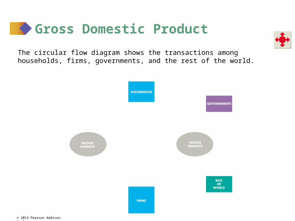
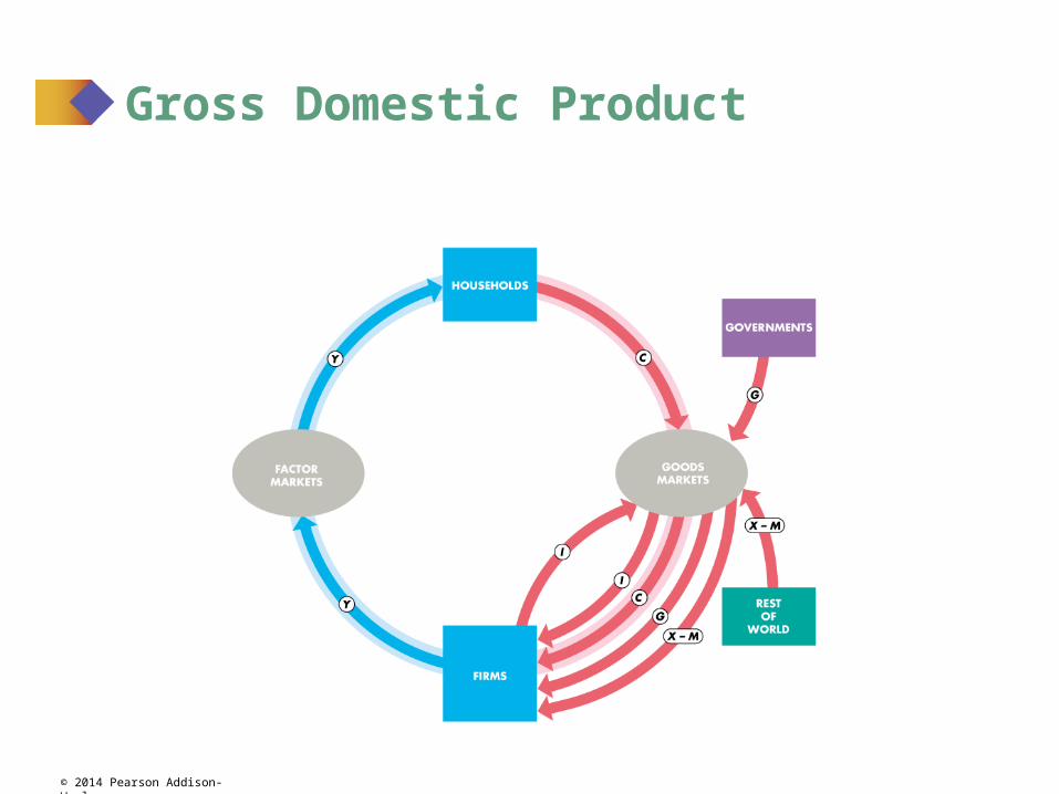
The circular flow diagram shows the transactions among households, firms, governments, and the rest of the world.



Households and Firms

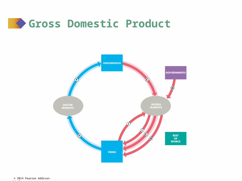
Households sell and firms buy the services of labor, capital, and land in factor markets.

For these factor services, firms pay income to households: wages for labor services, interest for the use of capital, and rent for the use of land. A fourth factor of production, entrepreneurship, receives profit.

In the figure, the blue flow, Y, shows total income paid by firms to households.



Firms sell and households buy consumer goods and services in the goods market.

Consumption expenditure is the total payment for consumer goods and services, shown by the red flow labeled C .

Firms buy and sell new capital equipment in the goods market and put unsold output into inventory.

The purchase of new plant, equipment, and buildings and the additions to inventories are investment, shown by the red flow labeled I.



Governments

Governments buy goods and services from firms and their expenditure on goods and services is called government expenditure.

Government expenditure is shown as the red flow G.

Governments finance their expenditure with taxes and pay financial transfers to households, such as unemployment benefits, and pay subsidies to firms.

These financial transfers are not part of the circular flow of expenditure and income.



Rest of the World

Firms in the United States sell goods and services to the rest of the world—exports—and buy goods and services from the rest of the world—imports.

The value of exports (X ) minus the value of imports (M) is called net exports, the red flow (X – M).

If net exports are positive, the net flow of goods and services is from U.S. firms to the rest of the world.

If net exports are negative, the net flow of goods and services is from the rest of the world to U.S. firms.


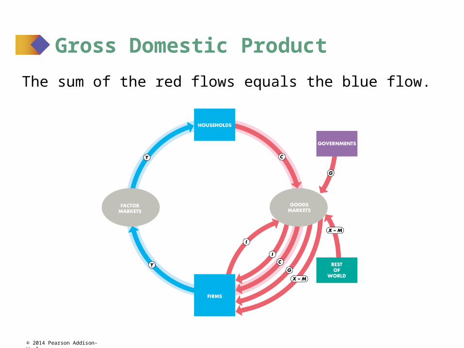
Gross Domestic Product The blue and red flows are the circular flow of expenditure and income.



The sum of the red flows equals the blue flow.



That is: Y = C + I + G + X – M



The circular flow shows two ways of measuring GDP.

GDP Equals Expenditure Equals Income

Total expenditure on final goods and services equals GDP.

GDP = C + I + G + X – M.

Aggregate income equals the total amount paid for the use of factors of production: wages, interest, rent, and profit.

Firms pay out all their receipts from the sale of final goods, so income equals expenditure,

Y = C + I + G + (X – M).



Why “Domestic” and Why “Gross”?

Domestic

Domestic product is production within a country.

It contrasts with national product, which is the value of goods and services produced anywhere in the world by the residents of a nation.

Gross

Gross means before deducting the depreciation of capital.

The opposite of gross is net, which means after deducting the depreciation of capital.



Depreciation is the decrease in the value of a firm’s capital that results from wear and tear and obsolescence.

Gross investment is the total amount spent on purchases of new capital and on replacing depreciated capital.

Net investment is the increase in the value of the firm’s capital.

Net investment = Gross investment Depreciation.



Gross investment is one of the expenditures included in the expenditure approach to measuring GDP.

So total product is a gross measure.

Gross profit, which is a firm’s profit before subtracting depreciation, is one of the incomes included in the income approach to measuring GDP.

So total product is a gross measure.


Measuring U.S. GDP

The Bureau of Economic Analysis uses two approaches to measure GDP:

The expenditure approach

The income approach


Measuring U.S. GDP

The Expenditure Approach

The expenditure approach measures GDP as the sum of consumption expenditure, investment, government expenditure on goods and services, and net exports.

GDP = C + I + G + (X M)

Table 4.1 on the next slide shows the expenditure approach with data (in billions) for 2012.

GDP = $11,007 + $2,032 + $3,055 $616

= $15,478 billion


Measuring U.S. GDP

The Income Approach

The income approach measures GDP by summing the incomes that firms pay households for the factors of production they hire—wages for labor, interest for capital, rent for land, and profit for entrepreneurship.


Measuring U.S. GDP

The National Income and Expenditure Accounts divide incomes into two broad categories:

1. Compensation of employees

2. Net operating surplus

Compensation of employees is the payments for labor services. It is the sum of net wages plus taxes withheld plus social security and pension fund contributions.

Net operating surplus is the sum of other factor incomes. It includes net interest, rental income, corporate profits, and proprietor’s income.


Measuring U.S. GDP

The sum of all factor incomes is net domestic income at factor cost.

Two adjustments must be made to get GDP:

1. Indirect taxes less subsidies are added to get from factor cost to market prices.

2. Depreciation is added to get from net domestic income to gross domestic income.

Table 4.2 on the next slide shows the income approach with data for 2012.


Measuring U.S. GDP

Nominal GDP and Real GDP

Real GDP is the value of final goods and services produced in a given year when valued at the prices of a reference base year.

Currently, the reference base year is 2005 and we describe real GDP as measured in 2005 dollars.

Nominal GDP is the value of goods and services produced during a given year valued at the prices that prevailed in that same year.

Nominal GDP is just a more precise name for GDP.


Measuring U.S. GDP

Calculating Real GDP

Table 4.3(a) shows the quantities produced and the prices in 2005 (the base year).

Nominal GDP in 2005 is $100 million.

Because 2005 is the base year, real GDP equals nominal GDP and is $100 million.


Measuring U.S. GDP

Table 4.3(b) shows the quantities produced and the prices in 2012.

Nominal GDP in 2012 is $300 million.

Nominal GDP in 2012 is three times its value in 2005.


Measuring U.S. GDP

In Table 4.3(c), we calculate real GDP in 2012.

The quantities are those of 2012, as in part (b).

The prices are those in the base year (2005) as in part (a).

The sum of these expenditures is real GDP in 2012, which is $160 million.


The Uses and Limitations of Real GDP

Economists use estimates of real GDP for two main purposes:

To compare the standard of living over time

To compare the standard of living across countries



The Standard of Living Over Time

Real GDP per person is real GDP divided by the population.

Real GDP per person tells us the value of goods and services that the average person can enjoy.

By using real GDP, we remove any influence that rising prices and a rising cost of living might have had on our comparison.



Long-Term Trend

A handy way of comparing real GDP per person over time is to express it as a ratio of some reference year.

For example, in 1960, real GDP per person was $15,850 and in 2012, it was $43,182.

So real GDP per person in 2012 was 2.7 times its 1960 level—that is, $43,182 ÷ $15,850 = 2.7.



Two features of our expanding living standard are

The growth of potential GDP per person

Fluctuations of real GDP around potential GDP

The value of real GDP when all the economy’s labor, capital, land, and entrepreneurial ability are fully employed is called potential GDP.



Figure 4.2 shows U.S. real GDP per person.

Potential GDP grows at a steady pace because the quantities of the factors of production and their productivity grow at a steady pace.

Real GDP fluctuates around potential GDP.



Real GDP per person in the United States:

Doubled between 1960 and 1990.

Was 2.7 times its 1960 level in 2012.



Productivity Growth Slowdown

The growth rate of real GDP per person slowed after 1970. How costly was that slowdown?

The answer is provided by a number that we’ll call the Lucas wedge.

The Lucas wedge is the dollar value of the accumulated gap between what real GDP per person would have been if the 1960s growth rate had persisted and what real GDP per person turned out to be.



Figure 4.3 illustrates the Lucas wedge.

The red line is actual real GDP per person.

The thin black line is the trend that real GDP per person would have followed if the 1960s growth rate of potential GDP had persisted.

The shaded area is the Lucas wedge.



Real GDP Fluctuations— The Business Cycle

A business cycle is a periodic but irregular up-and-down movement of total production and other measures of economic activity.

Every cycle has two phases:1. Expansion2. Recession

and two turning points:1. Peak2. Trough



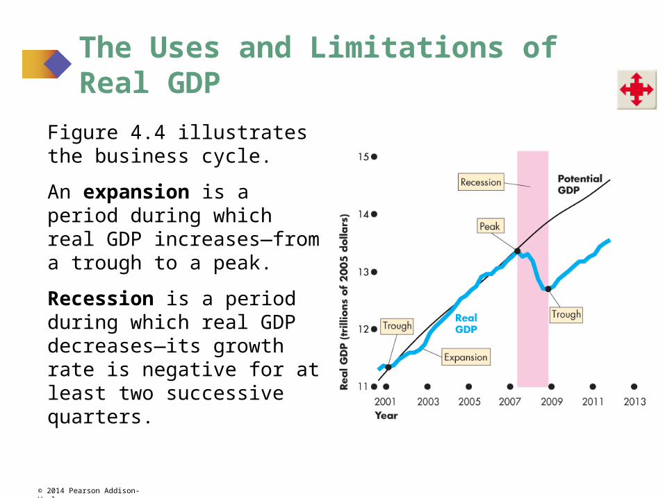
Figure 4.4 illustrates the business cycle.

An expansion is a period during which real GDP increases—from a trough to a peak.

Recession is a period during which real GDP decreases—its growth rate is negative for at least two successive quarters.



The Standard of Living Across Countries

Two problems arise in using real GDP to compare living standards across countries:

1. The real GDP of one country must be converted into the same currency units as the real GDP of the other

country.

2. The goods and services in both countries must be valued at the same prices.



Using the exchange rate to compare GDP in one country with GDP in another country is problematic because …

prices of particular products in one country may be much less or much more than in the other country.

For example, using the market exchange rate to value China’s GDP in U.S. dollars leads to an estimate that in 2012, GDP per person in the United States was 8.4 times GDP per person in China.



Figure 4.5 illustrates the problem.

Using the market exchange rate and domestic prices makes China look like a poor developing country.

But when GDP is valued at purchasing power parity prices, U.S. income per person is only 5.6 times that in China.



Limitations of Real GDP

Real GDP measures the value of goods and services that are bought in markets.

Some of the factors that influence the standard of living and that are not part of GDP are

Household production Underground economic activity Leisure time Environmental quality



The Bottom Line

Do we get the wrong message about the level and growth of economic well-being and the standard of living by looking at the growth of real GDP?

The influences that are omitted from real GDP are probably large.

It is possible to construct broader measures that combine the many influences that contribute to human happiness.

Despite all the alternatives, real GDP per person remains the most widely used indicator of economic well-being.


Mathematical Note: Chained-Dollar Real GDP

The BLS uses a measure of real GDP called chained-dollar real GDP.

Three steps are needed to calculate this measure:Value production in the prices of adjacent years Find the average of two percentage changesLink (chain) back to the reference year



Value Production in Prices of Adjacent Years

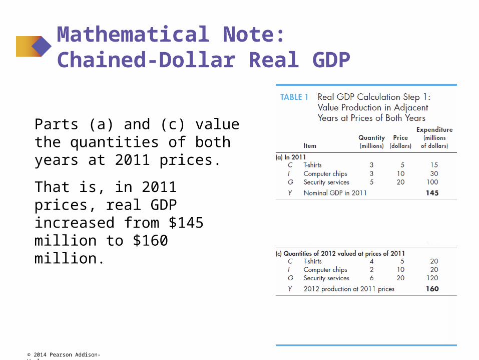
Part (a) shows the quantities and prices in 2011.

Part (b) shows the quantities and prices in 2012.

Part (c) the quantities of 2012 valued at 2011 prices.

Part (d) the quantities of 2011 valued at prices of 2012.



Parts (a) and (c) value the quantities of both years at 2011 prices.

That is, in 2011 prices, real GDP increased from $145 million to $160 million.



Parts (d) and (b) value the quantities in both years at 2012 prices.

That is, in 2012 prices, real GDP increased from $275 million to $300 million.



Find the Average of Two Percentage Changes

Part (a) shows that at 2011 prices, production increased by 10.3%.

Part (b) shows that at 2012 prices, production increased by 9.1%.

The average increase in production is 9.7%.



Link (Chain) to the Base Year

To find real GDP in 2012 in base-year prices (2005), we need to know the

1. Real GDP in 2005

2. Average growth rate each year from 2005 to 2012.

The BEA must calculate the percentage change of the growth rate in real GDP for each pair of years from the base year to the most recent year.

To find real GDP for years before the base year, the BEA must calculate the growth rates for each pair of years back to the earliest one available.


Finally, using the percentage changes that it has calculated, the BEA finds the real GDP in each year in 2005 prices by linking them to the GDP in 2005.

The figure shows an example.


Graphs in Macroeconomics


After studying this appendix, you will be able to:

Make and interpret a time-series graph

Make and interpret a graph that uses a ratio scale


Making a Time-Series Graph

A time-series graph measures

Time on the x-axis and

The variable in which we are interested on the y-axis.

The Time-Series Graph


Reading a Time-Series Graph

A time-series graph shows the

Level of the variable

Change in the variable

The speed of change in the variable



Ratio Scale Reveals Trend

A time-series graph also reveals whether a variable has a

Cycle—a tendency for a variable to alternate between upward and downward movements

Trend—a tendency for a variable to move in one general direction



This time-series graph has

A cycle

No trend



A Time-Series with a Trend

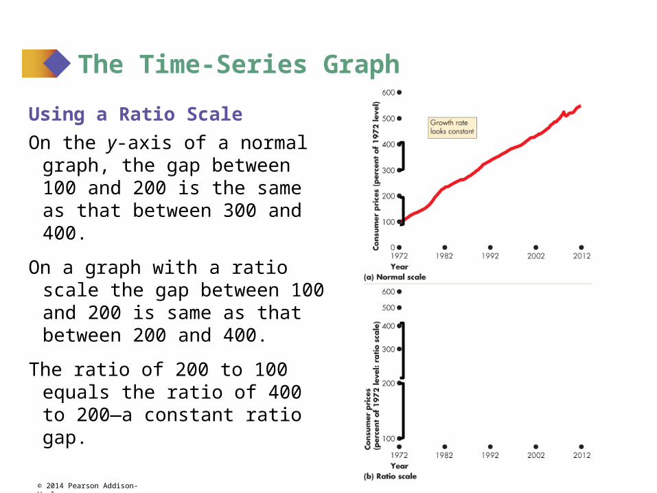
Figure A4.2(a) shows the average prices paid by consumers since 1972.

In 1972, the price is set at 100.

The price in other years is measured as a percentage of the 1972 level.

Prices look as if they rose at a fairly constant rate.



Using a Ratio Scale

On the y-axis of a normal graph, the gap between 100 and 200 is the same as that between 300 and 400.

On a graph with a ratio scale the gap between 100 and 200 is same as that between 200 and 400.

The ratio of 200 to 100 equals the ratio of 400 to 200—a constant ratio gap.



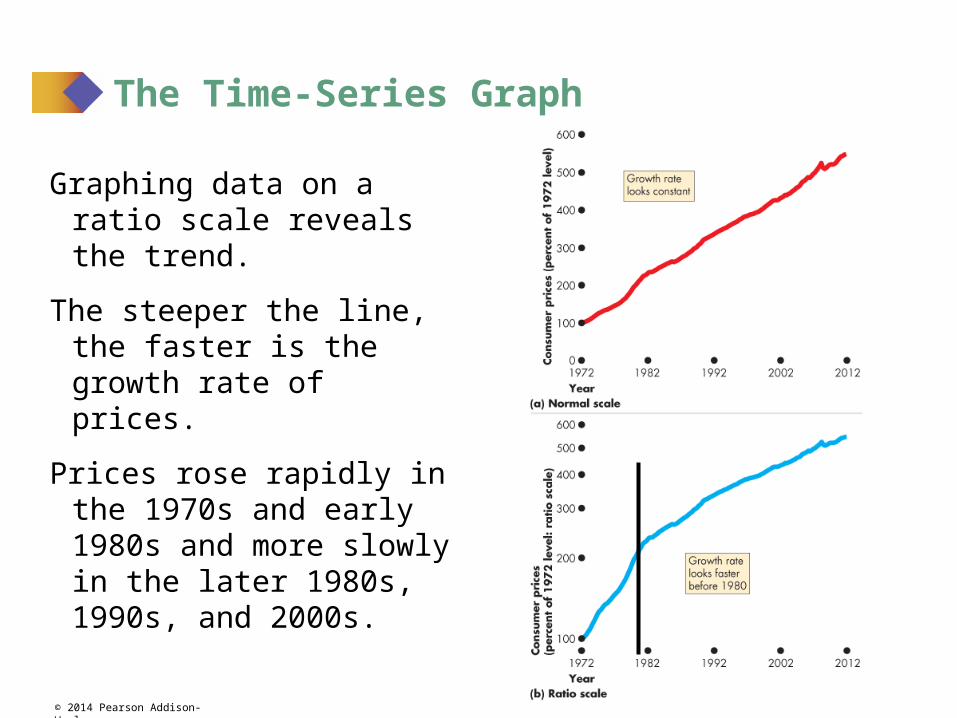
Graphing data on a ratio scale reveals the trend.

The steeper the line, the faster is the growth rate of prices.

Prices rose rapidly in the 1970s and early 1980s and more slowly in the later 1980s, 1990s, and 2000s.


4 MEASURING GDP AND ECONOMIC GROWTH © 2014 Pearson Addison-Wesley After studying this chapter, you...

Documents

Transcript of 4 MEASURING GDP AND ECONOMIC GROWTH © 2014 Pearson Addison-Wesley After studying this chapter, you...