4. Gaussian derivatives - midag.cs.unc.edumidag.cs.unc.edu/pubs/CScourses/254-Spring2002/04... ·...

In[3]:= << FEVinit`;

<< FEVFunctions`;

4. Gaussian derivatives

4.1 Introduction

We will encounter the Gaussian derivative function at many places throughout this book. Therefore

we discuss this function in quite some detail in this chapter. The Gaussian derivative function has

many interesting properties. We will discuss them in one dimension first. We study its shape and

algebraic structure, its Fourier transform, and its close relation to other functions like the Hermite

functions, the Gabor functions and the generalized functions. In two and more dimensions additional

properties are involved like orientation (directional derivatives) and anisotropy. We discuss these atthe end of this chapter.

4.2 Shape and algebraic structure

When we take derivatives to x (spatial derivatives) of the Gaussian function repetitively, we see a

pattern emerging of a polynomial of increasing order, multiplied with the original (normalized)

Gaussian function again. Here we show a table of the derivatives from order 0 (i.e. no differentiation)

to 3.

In[5]:= Unprotect@gaussD; gauss@x_, σ_D :=1

��σ

è!!!!!!!!!2 π

ExpA−x2

��2 σ2

E;In[6]:= Table@Factor@Evaluate@D@gauss@x, σD, 8x, n<DDD, 8n, 0, 3<DOut[6]= 9 ã− x2��

2 σ2

��è!!!!!!!!2 π σ

, −ã− x2��

2 σ2 x��è!!!!!!!!2 π σ3

,ã− x2��

2 σ2 Hx − σL Hx + σL��è!!!!!!!!

2 π σ5, −

ã− x2��2 σ2 x Hx2 − 3 σ2L

��è!!!!!!!!2 π σ7

=Ł The function Factor takes polynomial factors apart. The function gauss[x,σ] is part of the

standard set of functions (FEVFunctions.m) with this book, and protected. If we want to

modify the function, we must first Unprotect it.

The zeroth order derivative is indeed the Gaussian function itself. This is how the graphs of Gaussian

derivative functions look like, from order 0 up to order 7:

04 GaussianDerivatives.nb 1

In[7]:= GraphicsArray@Partition@Table@Plot@Evaluate@D@gauss@x, 1D, 8x, n<DD, 8x, −5, 5<,

PlotLabel −> StringJoin@"Order=", ToString@nDD, DisplayFunction −>

IdentityD, 8n, 0, 7<D, 4D, ImageSize −> 550D êê Show;

-4 -2 2 4-0.5

0.5

1

Order=4

-4 -2 2 4

-2

-1

1

2

Order=5

-4 -2 2 4

-6

-4

-2

2

4Order=6

-4 -2 2 4

-10

-5

5

10

Order=7

-4 -2 2 4

0.1

0.2

0.3

0.4Order=0

-4 -2 2 4

-0.2

-0.1

0.1

0.2

Order=1

-4 -2 2 4

-0.4

-0.3-0.2

-0.1

0.1

Order=2

-4 -2 2 4

-0.4

-0.2

0.2

0.4

Order=3

Figure 4.1. Plots of the Gaussian derivative function for order 0 to 7.

The even order (including the zeroth order) derivative functions are even functions (i.e. symmetric

around zero) and the odd order derivatives are odd functions (antisymmetric around zero). Note the

marked increase in amplitude for higher order of differentiation.

The Gaussian function itself is a common element of all higher order derivatives. We extract the

polynomials by dividing by the Gaussian function:

In[8]:= TableAEvaluateA D@gauss@x, σD, 8x, n<D��

gauss@x, σD E, 8n, 0, 4<E êê Simplify

Out[8]= 91, −x

��σ2

,x2 − σ2

��σ4

, −x3 − 3 x σ2

��σ6

,x4 − 6 x2 σ2 + 3 σ4��

σ8=

These polynomials have the same order as the derivative they are related to. Note that the highest

order of x is the same as the order of differentiation, and that we have a plus sign for the highest order

of x for even number of differentiation, and a minus signs for the odd orders.

These polynomials are the Hermite polynomials, called after Charles Hermite, a brilliant French

mathematician (see figure 4.2). They emerge from the following definition:∂ne-x2

��∂xn = H−1Ln Hn HxL e-x2 . The function Hn HxL is the Hermite polynomial, where n is called

the order of the polynomial. When we make the substitution x → x ê σ, we get the following relation

between the Gaussian function GHx, σL and its derivatives:

∂nGHx,σL��∂xn = H−1Ln 1��σn HnH x��σ L GHx, σL.


In[9]:= Show@Import@"Hermite.gif"D, ImageSize −> 155D;

Figure 4.2. Charles Hermite (1822-1901).

In Mathematica the function Hn is given by the function HermiteH[n,x]. Here are the Hermite

functions from zeroth to fifth order:

In[10]:= Table@HermiteH@n, xD, 8n, 0, 5<DOut[10]= 81, 2 x, −2 + 4 x2, −12 x + 8 x3, 12 − 48 x2 + 16 x4, 120 x − 160 x3 + 32 x5<The inner scale σ is introduced in the equation by substituting x → x��

σ è!!!!2 . As a consequence, with

each differentiation we get a new factor 1��σ è!!!!2 . So now we are able to calculate the 1-D Gaussian

derivative functions gd[x,n,σ] directly with the Hermite polynomials, again incorporating the

normalization factor 1��σ è!!!!!!!!2 π

:

In[11]:= gd@x_, n_, σ_D :=ikjjjjj −1

��σ

è!!!!2

y{zzzzzn

HermiteHAn, x��σ

è!!!!2

E 1��σ

è!!!!!!!!2 π

ExpA−x2

��2 σ2

ECheck:

In[12]:= FullSimplify@gd@x, 4, σD, σ > 0DOut[12]=

ã− x2��2 σ2 Hx4 − 6 x2 σ2 + 3 σ4L

��è!!!!!!!!2 π σ9

In[13]:= FullSimplifyADA 1��σ

è!!!!!!!!2 π

ExpA−x2

��2 σ2

E, 8x, 4<E, σ > 0EOut[13]=

ã− x2��2 σ2 Hx4 − 6 x2 σ2 + 3 σ4L

��è!!!!!!!!2 π σ9


The amplitude of the Hermite polynomials explodes for large x, but the Gaussian envelop suppresses

any polynomial function. No matter how high the polynomial order, the exponential function always

wins. We can see this graphically when we look at e.g. the 7th order Gaussian derivative without (i.e.

the Hermite function, figure left) and with its Gaussian weight function (figure right). Note the vertical

scales:

In[14]:= BlockA8$DisplayFunction = Identity<,p1 =

PlotAikjjjjj 1��è!!!!2

y{zzzzz7

HermiteHA7, x��è!!!!2

E, 8x, −5, 5<, PlotRange −> 8−800, 800<E;p2 = PlotAikjjjjj 1

��è!!!!2

y{zzzzz7

HermiteHA7, x��è!!!!2

E ExpA−x2��2

E,8x, −5, 5<, PlotRange −> AllE;E

Show@GraphicsArray@8p1, p2<D, ImageSize −> 8450, 130<D;

-4 -2 2 4

-750

-500

-250

250

500

750

-4 -2 2 4

-30

-20

-10

10

20

30

Figure 4.3. Left: The 7th order Hermite polynomial. Right: idem, with a Gaussian envelop (weightingfunction). This is the 7th order Gaussian derivative kernel.

Due to the limiting extent of the Gaussian window function, the amplitude of the Gaussian derivative

function can be negligeable at the location of the larger zeros. We plot an example, showing the 20th

order derivative and its Gaussian envelope function:


In[16]:= << Graphics`FilledPlot`; n = 20; σ = 1;

BlockA8$DisplayFunction = Identity<,p1 = FilledPlot@gd@x, n, σD, 8x, −5, 5<, PlotRange → AllD;p2 = PlotA gd@0, n, σD gauss@x, σD

��gauss@0, σD , 8x, −5, 5<, PlotRange → AllEE;

Show@8p1, p2<, ImageSize → 8320, 200<,DisplayFunction −> $DisplayFunctionD;

-4 -2 2 4

-2 µ 108

-1 µ 108

1 µ 108

2 µ 108

-4 -2 2 4

-2 µ 108

-1 µ 108

1 µ 108

2 µ 108

Figure 4.4. The 20th order Gaussian derivative's outer zero-crossings vahish in negligence. Notealso that the amplitude of the Gaussian derivative function is not bounded by the Gaussian window.

The Gaussian function is at x = 3 σ, x = 4 σ and x = 5 σ, relative to its peak value:

In[19]:= TableA gauss@σ, 1D��gauss@0, 1D , 8σ, 3, 5<E êê N

Out[19]= 80.011109, 0.000335463, 3.72665 × 10−6<and in the limit:

In[20]:= Limit@gd@x, 7, 1D, x −> InfinityDOut[20]= 0

The Hermite polynomials belong to the family of orthogonal functions on the infinite interval (-

∞,∞) with the weight function e− x2��2 , i.e. Ÿ−∞

∞e− x2��2 HnHxL HmHxL âx = è!!!!!!!!2 π n! δnm , where

δnm is the Kronecker delta, or delta tensor. δnm = 1 for n = m, and δnm = 0 for n ≠ m. The

Gaussian derivative functions, with their weight function e− x2��4 are not orthogonal. Other families of

orthogonal polynomials are e.g. Legendre, Chebyshev, Laguerre, and Jacobi polynomials. Other

orthogonal families of functions are e.g. Bessel functions and the spherical harmonic functions.

Note that the area under the Gaussian derivative functions is not unity, e.g. for the first derivative:


In[21]:= SetOptions@Integrate, GenerateConditions −> FalseD;‡0

∞

gd@x, 1, σD âx

Out[22]= −1

��è!!!!!!!!2 π

4.3 Gaussian Derivatives in the Fourier Domain

The Fourier transform of the derivative of a function is H−i ωL times the Fourier transform of the

function. For each differentiation, a new factor H−i ωL is added. So the Fourier transforms of the

Gaussian function and its first and second order derivative are:

In[23]:= σ =.; FullSimplify@FourierTransform@8gauss@x, σD, ∂xgauss@x, σD, ∂8x,2<gauss@x, σD<, x, ωD, σ > 0DOut[23]= 9 ã− 1��2 σ2 ω2

��è!!!!!!!!2 π

, −ä ã− 1��2 σ2 ω2 ω��è!!!!!!!!

2 π, −

ã− 1��2 σ2 ω2 ω2

��è!!!!!!!!2 π

=In general: F 8 ∂nGHx,σL��∂xn < = H−iωLn F 8GHx, σL<.

Gaussian derivative kernels also act as bandpass filters. The maximum amplitude is reached at

ω = è!!!!n :

In[24]:= n =.; σ = 1; SolveAEvaluateADA H−I ωLn

��è!!!!!!!!2 π

ExpA−σ2 ω2

��2

E, ωEE == 0, ωEOut[24]= 99ω → ä 0

1��n =, 9ω → −è!!!!n =, 9ω →

è!!!!n ==

The normalized powerspectra show that higher order of differentiation means a higher center

frequency for the bandpass filter. The bandwidth remains virtually the same.


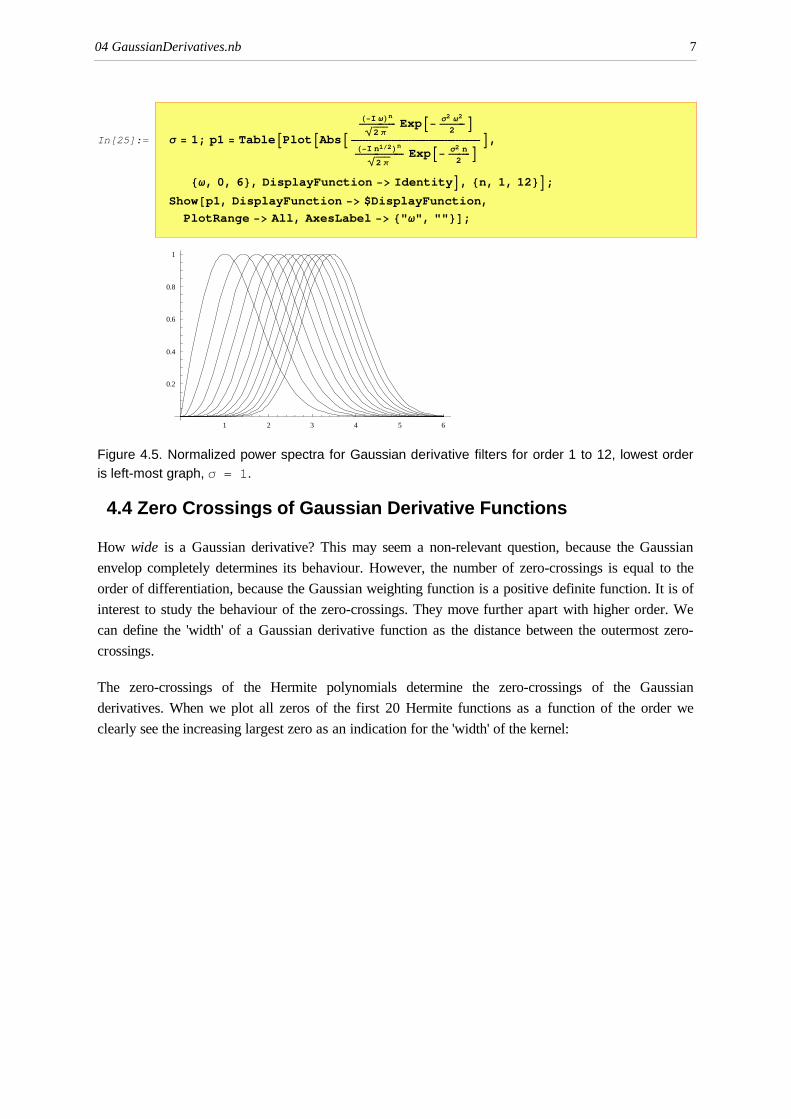
In[25]:= σ = 1; p1 = TableAPlotAAbsA H−I ωLn��è!!!!!!!2 π

ExpA− σ2 ω2��2

E��H−I n1ê2Ln��è!!!!!!!

2 πExpA− σ2 n��

2E E,

8ω, 0, 6<, DisplayFunction −> IdentityE, 8n, 1, 12<E;Show@p1, DisplayFunction −> $DisplayFunction,

PlotRange −> All, AxesLabel −> 8"ω", ""<D;

1 2 3 4 5 6w

0.2

0.4

0.6

0.8

1

Figure 4.5. Normalized power spectra for Gaussian derivative filters for order 1 to 12, lowest orderis left-most graph, σ = 1.

4.4 Zero Crossings of Gaussian Derivative Functions

How wide is a Gaussian derivative? This may seem a non-relevant question, because the Gaussian

envelop completely determines its behaviour. However, the number of zero-crossings is equal to the

order of differentiation, because the Gaussian weighting function is a positive definite function. It is of

interest to study the behaviour of the zero-crossings. They move further apart with higher order. We

can define the 'width' of a Gaussian derivative function as the distance between the outermost zero-

crossings.

The zero-crossings of the Hermite polynomials determine the zero-crossings of the Gaussian

derivatives. When we plot all zeros of the first 20 Hermite functions as a function of the order we

clearly see the increasing largest zero as an indication for the 'width' of the kernel:


In[27]:= gd@x_, n_, σ_D :=ikjjjjj −1

��σ

è!!!!2

y{zzzzzn

HermiteHAn, x��σ

è!!!!2

E 1��σ

è!!!!!!!!2 π

ExpA−x2

��2 σ2

E;nmax = 20; σ = 1;

[email protected], Point @8n, x<D< ê.SolveAHermiteHAn, x

��è!!!!2

E == 0, xE, 8n, 1, nmax<E, 1EE,AxesLabel −> 8"Order", "Zeros of\nHermiteH"<, Axes −> TrueE;

5 10 15 20Order

-7.5

-5

-2.5

2.5

5

7.5

Zeros of

HermiteH

Figure 4.6. Zero crossings of Gaussian derivative functions to 20th order. Each dot is a zero-crossing.

Note that the zeros of the second derivative are just one standard deviation from the origin:

In[29]:= σ =.; Simplify@Solve@D@gauss@x, σD, 8x, 2<D == 0, xD, σ > 0DOut[29]= 88x → −σ<, 8x → σ<<An exact analytic solution for the largest zero is not known. The formula of Zernicke (1931) specifies

a range, and Szego (1939) gives a better estimate:


In[30]:= BlockA8$DisplayFunction = Identity<,p1 = PlotA2 SqrtAn + 1 − 3.05

è!!!!!!!!!!!!n + 1

3 E, 8n, 5, 50<E;H∗ Zernicke upper limit ∗Lp2 = PlotA2 SqrtAn + 1 − 1.15

è!!!!!!!!!!!!n + 1

3 E, 8n, 1, 50<E;H∗ Zernicke lower limit ∗Lp3 = PlotA2 è!!!!!!!!!!!!!!

n + .5 − 2.338098 í è!!!!!!!!!!!!!!n + .5

6,8n, 1, 50<, PlotStyle −> [email protected], .02<DEE;

Show@8p1, p2, p3<, AxesLabel −>8"Order", "Width of Gaussian\nderivative Hin σL"<D;

10 20 30 40 50Order

2

4

6

8

10

12

14

Width of Gaussian

derivative Hin sL

Figure 4.7. Estimates for the width of Gaussian derivative functions to 50th order. Width is definedas the distance between the outmost zero-crossings. Top and bottom graph: estimated range byZernicke (1931), dashed graph: estimate by Szego (1939)

For very high orders of differentiation of course the numbers of zero-crossings increases, but also

their mutual distance between the zeros becomes more equal. In the limiting case of infinite order the

Gaussian derivative function becomes a sinusoidal function:

limnz∞∂n G��∂n x Hx, σL = Sin Jx "#####################1��σ H n+1��2 L N.

4.5 The correlation between Gaussian Derivatives

Higher order Gaussian derivative kernels tend to become more and more similar. Compare e.g. the

20th and 24nd derivative function:


In[32]:= Block@8$DisplayFunction = Identity<,g1 = Plot@gd@x, 20, 2D, 8x, −7, 7<, PlotLabel −> "Order 20"D;g2 = Plot@gd@x, 24, 2D, 8x, −7, 7<, PlotLabel −> "Order 24"DD;

Show@GraphicsArray@8g1, g2<, ImageSize −> 8480, 140<DD;

-6 -4 -2 2 4 6

-100

-50

50

100

Order 20

-6 -4 -2 2 4 6

-3000

-2000

-1000

1000

2000

3000

Order 24

Figure 4.8. Gaussian derivative functions start to look more and more alike for higher order. Herethe graphs are shown for the 20th and 24th order of differentiation.

This makes them not very suitable as a basis. But before we investigate their role in a possible basis,let us investigate their similarity. In fact we can express exactly how much they resemble each other

as a function of the difference in differential order, by calculationg the correlation between them. We

derive the correlation below, and will appreciate the nice mathematical properties of the Gaussian

function. Because the higher dimensional Gaussians are just the product of 1D Gaussian functions, it

suffices to study the 1D case.

The correlation coefficient between two functions is defined as the integral of the product of the

functions over the full domain (in this case -∞ to +∞). Because we want the coefficient to be unity for

complete correlation (when the functions are identical by an amplitude scaling factor) we divide the

coefficient by the so-called autocorrelation coefficients, i.e. the correlation of the functions with

themself. We then get as definition for the correlation coefficient r between two Gaussian derivatives

of order n and m:

(1)rn,m =Ÿ−∞

∞gHnLHxL gHmLHxL âx

��"###########################################################################Ÿ−∞

∞ @gHnLHxLD2 âx Ÿ−∞

∞ @gHmLHxLD2 âx

with gHnLHxL = ∂ng HxL��∂ xn . The Gaussian kernel gHxL itself is an even function, and, as we have

seen before, gHnLHxL is an even function for n is even, and an odd function for n is odd. The

correlation between an even function and an odd function is zero. This is the case when n and m are

both not even or both not odd, i.e. when Hn − mL is odd. We now can see already two important

results:

rn,m = 0 for Hn − mL odd;

rn,m = 1 for n = m .

The remaining case is when Hn − mL is even. We take n > m. Let us first look to the

nominator,Ÿ−∞

∞gHnLHxL gHmLHxL âx. The standard approach to tackle high exponents of functions

in integrals, is the reduction of these exponents by partial integration:


Ÿ−∞

∞gHnLHxL gHmLHxL âx = gHnLHxL gHmLHxL »−∞

∞ −Ÿ−∞

∞gHn−1LHxL gHm+1LHxL âx =H−1Lk Ÿ−∞

∞gHn−kLHxL gHm+kLHxL âx

when we do the partial integration k times. The 'stick expression' gHnLHxL gHmLHxL »−∞∞ is zero

because any Gaussian derivative function goes to zero for large x. We can choose k such that the

exponents in the integral are equal (so we end up with the square of a Gaussian derivative function).

So we make Hn − kL = Hm + kL, i.e. k = Hn−mL��2 . Because we study the case that Hn − mL is even,

k is an integer number. We then get:H−1Lk Ÿ−∞

∞gHn−kLHxL gHm+kLHxL âx = H−1L n−m��2 Ÿ−∞

∞gH n+m��2 LHxL gH n+m��2 LHxL âx

The total energy of a function in the spatial domain is the integral of the square of the function over

its full extent. The famous theorem of Parceval states that the total energy of a function in the spatial

domain is equal to the total energy of the function in the Fourier domain, i.e. expressed as the integral

of the square of the Fourier transform over its full extent. Therefore

H−1L n−m��2 Ÿ−∞

∞gH n+m��2 LHxL gH n+m��2 LHxL âx =ParcevalH−1L n−m��2 1��2 π Ÿ−∞

∞ … HiωL n+m��2 g HωL …2 âω =H−1L n−m��2 1��2 π Ÿ−∞

∞ωn+m g2 HωL âω = H−1L n−m��2 1��2 π Ÿ−∞

∞ωn+m e−σ2 ω2

â ω

We now substitute ω' = σω, and get finally: H−1L n−m��2 1��2 π 1��σn+m+1 Ÿ−∞

∞ω'Hn+mL e−ω'2 âω'.

This integral can be looked up in a table of integrals, but why not let Mathematica do the job (we first

clear n and m):

In[34]:= n =.; m =.; ‡−∞

∞

xm+n e−x2 âx

Out[34]=1��2

H1 + H−1Lm+nL GammaA 1��2

H1 + m + nLE Log@eD 1��2 H−1−m−nLThe function Gamma is the Euler gamma function. In our case Re[m+n]>-1, so we get for our

correlation coefficient for Hn − mL even:

rn,m =H−1L n−m��2 1��2 π 1��

σn+m+1 ΓH m+n+1��2 L��"#####################################################################################1��2 π 1��

σ2 n+1 ΓH 2 n+1��2 L 1��2 π 1��σ2 m+1 ΓH 2 m+1��2 L = H−1L n−m��2 ΓH m+n+1��2 L��"########################################ΓH 2 n+1��2 L ΓH 2 m+1��2 L

With this function we can study the correlation behaviour for large n and m quite easily. Let's first

have a look at this function tabulated for a range of values for small n and m (0-7):


In[35]:= r@n_, m_D := H−1L n−m��2 GammaA m + n + 1��

2E ì $%%%%%%%%%%%%%%%%%%%%%%%%%%%%%%%%%%%%%%%%%%%%%%%%%%%%%%%%%%%%%%%%%%%%%%%%%%%GammaA 2 n + 1

��2

E GammaA 2 m + 1��

2E ;

Table@NumberForm@r@n, mD êê N, 3D, 8n, 0, 5<, 8m, 0, 5<D êê MatrixForm

Out[36]//MatrixForm=i

kjjjjjjjjjjjjjjjjjjjj

1. 0. − 0.798 ä −0.577 0. + 0.412 ä 0.293 0. − 0.208 ä

0. + 0.798 ä 1. 0. − 0.921 ä −0.775 0. + 0.623 ä 0.488−0.577 0. + 0.921 ä 1. 0. − 0.952 ä −0.845 0. + 0.719 ä

0. − 0.412 ä −0.775 0. + 0.952 ä 1. 0. − 0.965 ä −0.8820.293 0. − 0.623 ä −0.845 0. + 0.965 ä 1. 0. − 0.973 ä

0. + 0.208 ä 0.488 0. − 0.719 ä −0.882 0. + 0.973 ä 1.

y

{zzzzzzzzzzzzzzzzzzzz

In[37]:= ListPlot3D@Table@Abs@r@n, mDD, 8n, 0, 15<, 8m, 0, 15<D,Axes −> True, AxesLabel −> 8"n", "m", "Abs\nr@n,mD"<,ViewPoint −> 8−2.348, −1.540, 1.281<D;

5

10

15n

5

10

15

m

0

0.25

0.5

0.75

1

Absr@n,mD

0

0.25

0.5

0.75

1

Absr@n,mD

Figure 3.9. The magnitude of the correlation coefficient of Gaussian derivative functions for0 < n < 15 and 0 < m < 50. The origin is in front.

The correlation is unity when n = m, as expected, is negative when n − m = 2, and is positive when

n − m = 4, and is complex otherwise. Indeed we see that when n − m = 2 the functions are even but

of opposite sign:

In[38]:= Block@8$DisplayFunction = Identity<,p1 = Plot@gd@x, 20, 2D, 8x, −5, 5<, PlotLabel −> "Order 20"D;p2 = Plot@gd@x, 22, 2D, 8x, −5, 5<, PlotLabel −> "Order 22"DD;

Show@GraphicsArray@8p1, p2<, ImageSize −> 8480, 140<DD;

-4 -2 2 4

-100

-50

50

100

Order 20

-4 -2 2 4

-600

-400

-200

200

400

600Order 22


Figure 4.10. Gaussian derivative functions differing two orders are of opposite polarity.

and when n − m = 1 they have a phase-shift, leading to a complex correlation coefficient:

In[40]:= Block@8$DisplayFunction = Identity<,p1 = Plot@gd@x, 20, 2D, 8x, −5, 5<, PlotLabel −> "Order 20"D;p2 = Plot@gd@x, 21, 2D, 8x, −5, 5<, PlotLabel −> "Order 21"DD;

Show@GraphicsArray@8p1, p2<, ImageSize −> 8480, 140<DD;

-4 -2 2 4

-100

-50

50

100

Order 20

-4 -2 2 4

-200

-100

100

200

Order 21

Figure 4.11. Gaussian derivative functions differing one order display a phase shift.

Of course, this is easy understood if we realize the factor H−i ωL in the Fourier domain, and that

i = e−i π��2 . We plot the behaviour of the correlation coefficient of two close orders for large n. The

asymptotic behaviour towards unity for increasing order is clear.

In[41]:= Plot@−r@n, n + 2D, 8n, 1, 20<, DisplayFunction −> $DisplayFunction,

AspectRatio −> .4, PlotRange −> 8.8, 1.01<,AxesLabel −> 8"Correlation\ncoefficient", "Order"<D;

5 10 15 20

Correlation

coefficient

0.8

0.85

0.9

0.95

Order

Figure 4.12. The correlation coefficient between a Gaussian derivative function and its evenneighbour up quite quickly tends to unity for high differential order.

4.6 Discrete Gaussian Kernels

Lindeberg [Lindeberg1990] derived the optimal kernel for the case when the Gaussian kernel was

discretized and came up with the "modified Bessel function of the first kind". In Mathematica this

function is available as BesselI.

The "modified Bessel function of the first kind" BesselI is almost equal to the Gaussian kernel for

σ > 1, as we see below. Note that the Bessel function has to be normalized by its value at x = 0.

For larger σ the kernels become rapidly very similar.


In[42]:= σ = 2;

PlotA9 1��è!!!!!!!!!!!!!!2 π σ2

ExpA −x2��2 σ2

E, 1��è!!!!!!!!!!!!!!2 π σ2

BesselI@x, σ2D ê BesselI@0, σ2D=,8x, 0, 8<, PlotStyle → 8RGBColor@1, 0, 0D, RGBColor@0, 0, 0D<,PlotLegend → 8"Gauss", "Bessel"<, LegendPosition → 81, 0<,LegendLabel → "σ = 2", PlotRange → All, ImageSize → 8330, 166<E;

2 4 6 8

0.05

0.1

0.15

0.2

Bessel

Gauss

s = 2

4.7 Higher dimensions and separability

Gaussian derivative kernels of higher dimensions are simply made by multiplication. Here again we

see the separability of the Gaussian, i.e. this is the separability. The function

gd2D@x, y, n, m, σx, σyD is an example of a Gaussian partial derivative function in 2D, first

order derivative to x, second order derivative to y, at scale 2 (equal for x and y):

In[44]:= gd2D@x_, y_, n_, m_, σx_, σy_D := gd@x, n, σxD gd@y, m, σyD;Plot3D@gd2D@x, y, 1, 2, 2, 2D, 8x, −7, 7<,8y, −7, 7<, AxesLabel −> 8x, y, ""<, PlotPoints −> 40,

PlotRange −> All, Boxed −> False, ImageSize −> 8250, 140<D;

Figure 4.13. Plot of ∂3GHx,yL��∂x ∂y2 . The two-dimensional Gaussian derivative function can be constructed

as the product of two one-dimensional Gaussian derivative functions., and so for higher dimensions,due to the separability of the Gaussian kernel for higher dimensions.

The ratio σx��σyis called the anisotropy ratio. When it is unity, we have an isotropic kernel, which

diffuses in the x and y direction by the same amount. The Greek word ισος means 'equal', τροπος

means 'direction' (τοπος means 'location, place').


4.8 Directional derivatives and steerable filters

4.9 Other families of kernels

The derivation given above required first principles be plugged in that essentially stated "we know

knothing" (at this stage of the observation). Of course, we can relax these principles, and introduce

some knowledge. When we want to derive a set of apertures tuned to a specific spatial frequency k”

in

the image, we add this physical quantity to the matrix of the dimensionality analysis:

In[46]:= m = 881, −1, −2, −2, −1<, 80, 0, 1, 1, 0<<;TableForm@m,TableHeadings −> 88"meter", "candela"<, 8"σ", "ω", "L0", "L", "k"<<DNullSpace@mD

Out[47]//TableForm=

σ ω L0 L kmeter 1 −1 −2 −2 −1candela 0 0 1 1 0

Out[48]= 881, 0, 0, 0, 1<, 80, 0, −1, 1, 0<, 81, 1, 0, 0, 0<<Following the exactly similar line of reasoning, we end up from this new set of constraints with a new

family of kernels, the Gabor family of receptive fields, with are given by a sinusoidal function (at the

specified spatial frequency) under a Gaussian window. In the Fourier domain:

GaborHω, σ, kL = e−ω2 σ2 ei k ω, which translates into the spatial domain:

In[49]:= gabor@x_, σ_D := Sin@xD 1��è!!!!!!!!!!!!!!2 π σ2

ExpA−x2

��2 σ2

E;The Gabor function model of cortical receptive fields was first proposed by Marcelja in 1980

[Marcelja1980]. However the functions themselves are often credited to Gabor [Gabor1946] who

supported their use in communications.

Gabor functions are defined as the sinus function under a Gaussian window with scale σ. The phase φ

of the sinusoidal function determines its detailed behaviour, e.g. for φ = π ê 2 we get an even function.


In[50]:= gabor@x_, φ_, σ_D := Sin@x + φD gauss@x, σD;Block@8$DisplayFunction = Identity<,

p1 = Plot@gabor@x, 0, 10D, 8x, −30, 30<, PlotRange −> 8−.04, .04<D;p2 = Plot@gabor@x, π ê 2, 10D, 8x, −30, 30<, PlotRange −> 8−.04, .04<D;p3 = Plot@gauss@x, 10D, 8x, −30, 30<, PlotRange −> 8−.04, .04<D;p13 = Show@p1, p3D; p23 = Show@p2, p3DD;

Show@GraphicsArray@8p13, p23<D, ImageSize −> 8480, 140<D;

-30 -20 -10 10 20 30

-0.04

-0.02

0.02

0.04

-30 -20 -10 10 20 30

-0.04

-0.02

0.02

0.04

Figure 3.14. Gabor functions are sinusoidal functions with a Gaussian envelope. Left: Sin[x]

G[x,10]; right: Sin[x+π/2] G[x,10].

Gabor functions can look very much like Gaussian derivatives, but they are not the same:

- Gabor functions have an infinite number of zero-crossings on their domain.

- The amplitudes of the sinusoidal function never exceeds the Gaussian envelope.

They can be made to look very similar by an appropriate choice of parameters:

In[53]:= gauss@x_, σ_D :=1

��è!!!!!!!!!!!!!!2 π σ2

ExpA−x2

��2 σ2

E;p1 = Plot@− gabor@x, 1D, 8x, −4, 4<,

PlotStyle → [email protected], 0.02<D, DisplayFunction → IdentityD;p2 = Plot@Evaluate@D@gauss@x, 1D, xDD, 8x, −4, 4<,

DisplayFunction → IdentityD;Show@8p1, p2<, DisplayFunction → $DisplayFunctionD;

-4 -2 2 4

-0.2

-0.1

0.1

0.2

Figure 3.15. Gabor functions can be made very similar to Gaussian derivative kernels. In a practicalapplication then there is no difference in result. Dotted graph: Gaussian first derivative kernel.


Continuous graph: Minus the Gabor kernel with the same σ as the Gaussian kernel. Note the

necessity of sign change due to the polarity of the sinusoidal function.

By relaxing or modifying other constraints, we might find other families of kernels (see e.g.

[Pauwels1995]).

We conclude this section by the realization that the front-end visual system at the retinal level must be

uncommitted, no feedback from higher levels is at stake, so the Gaussian kernel seems a good

candidate to start observing with at this level. At higher levels this constraint is released. The

extensive feedback loops from the primary visual cortex to the LGN may give rise to 'geometry-driven

diffusion' [terHaarRomeny1994c], nonlinear scale-space theory, where the early differential geometric

measurements through e.g. the simple cells may modify the kernels LGN levels. Nonlinear scale-spacetheory will be treated in chapter 19.

ò [Task 3.1] When we have noise in the signal to be differentiated, we havetwo counterbalancing effect when we change differential order andscale: for higher order the noise is amplified (the factor H−i ωLn in theFourier transform representation) and the noise is averaged out forlarger scales. Give an explicit formula in our Mathematica framework forthe propagation of noise when filtered with Gaussian derivatives. Startwith the easiest case, i.e. pixel-uncorrelated noise, and continue withcorrelated noise. See for a treatment of this subject the work by HansBlom et al. [Blom1993a].

ò [Task 3.2] Give an explicit formula in our Mathematica framework for thepropagation of noise when filtered with a compound function ofGaussian derivatives, e.g. by the Laplacean ∂2G��∂x2 + ∂2G��∂y2 . See for a

treatment of this subject the work by Hans Blom et al. [Blom1993a].


4. Gaussian derivatives - midag.cs.unc.edumidag.cs.unc.edu/pubs/CScourses/254-Spring2002/04... ·...

Documents

Transcript of 4. Gaussian derivatives - midag.cs.unc.edumidag.cs.unc.edu/pubs/CScourses/254-Spring2002/04... ·...