4 ds C- 2: Unit C - 1: List of Subjects
47
AE301 Aerodynamics I UNIT C: 2-D Airfoils ROAD MAP . . . C-1: Aerodynamics of Airfoils 1 C-2: Aerodynamics of Airfoils 2 C-3: Panel Methods C-4: Thin Airfoil Theory Unit C-1: List of Subjects Wings and Airfoils Lift Curves Airfoils NACA Conventional Airfoils NACA Airfoil Data
Transcript of 4 ds C- 2: Unit C - 1: List of Subjects

AE301 Aerodynamics I
UNIT C: 2-D Airfoils
ROAD MAP . . .
C-1: Aerodynamics of Airfoils 1
C-2: Aerodynamics of Airfoils 2
C-3: Panel Methods
C-4: Thin Airfoil Theory
AE301 Aerodynamics I
Unit C-1: List of Subjects
Wings and Airfoils
Lift Curves
Airfoils
NACA Conventional Airfoils
NACA Airfoil Data
NOMENCLATURE FOR WINGS (3-D)
3-D Wing Geometry Nomenclature:
• Leading edge (LE)
• Trailing Edge (TE)
• Airfoil (a cross section of wing)
Recall that the lift, drag, and moment coefficient for 3-D wing can be defined as:
L
LC
q S
= D
DC
q S
= M
MC
q Sc
=
NOMENCLATURE FOR AIRFOILS (2-D)
2-D Airfoil Geometry Nomenclature:
• Chord Line
• Mean Camber Line
• Chord (c)
• Thickness (t)
• Camber: (difference between chord line and mean camber line)
For 2-D airfoil, the aerodynamic coefficients are “per unit span” basis:
( )
( )'
1l
L b Lc
q c q c
= = ( )
( )'
1d
D b Dc
q c q c
= = ( )
( ) 2
'
1m
M b Mc
q cq c c
= =
Note: b = wing span
Unit C-1Page 1 of 10
Wings and Airfoils
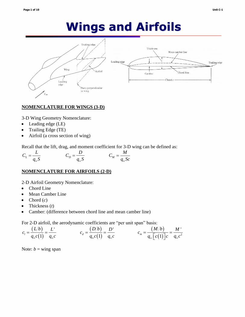
LIFT OF AIRFOILS
Lift on an airfoil depends on the following properties:
• V (freestream velocity)
• (freestream density)
• S (wing area)
Hence, lift coefficients are normalized by these properties: L
LC
q S
= and '
l
Lc
q c
= .
LIFT CURVE OF AIRFOILS
The behavior of lift (“lift curve” characteristics) depends on the following properties:
• (angle of attack)
Lift-curve (or often called, “cl - ” curve) provides important relationship between angle of attack and
lift coefficient, under a certain condition of Reynolds number. Interestingly, lift-curve is fairly close to a
linear line, as long as it is not under the “stall” condition (hence, we often assume it is a simple “linear
function” in our aerodynamic analysis for simplification).
• (viscosity)
Lift curve depends on the Reynolds number.
• a (freestream speed of sound, or “compressibility”)
Lift curve will also depend on the compressibility of the flow field (Mach number).
Unit C-1Page 2 of 10
Lift Curves

AIRFOILS
• The “shape” of airfoil: the design of 2-D airfoil will have a significant impact on aircraft
performance.
• Airfoils represent performance of a given cross-section of a wing. The shape of an airfoil has
tremendous effects on the overall performance of wing (thus, airplane).
• Airfoils can be considered as a model for a “unit span” of an infinite wing of constant cross-
section. The performance of an airfoil can be determined by a “quasi-2-D” wind tunnel tests.
• A Quasi-2-D is actually a 3-D, but constant cross section. Thus, the cross-sectional properties (i.e.,
lift, drag, and moment “per unit length”) can be determined.
GEOMETRIC AND AERODYNAMIC TWISTS OF WINGS
• Geometric twist of wing is varying angle of attack along the span, but retains the same airfoil.
• Aerodynamic twist of wing is varying airfoil (cross section of the wing) along the span, but retains
the angle of attack.
Unit C-1Page 3 of 10
Airfoils (1)
http://www.ae.uiuc.edu/m-selig/ads.html

CAMBERED V.S. SYMMETRICAL AIRFOIL
The camber in airfoil is the asymmetry between the top and the bottom curves of an airfoil. Cambered
airfoils generate lift at positive, zero, or even small negative angle of attack, whereas a symmetric airfoil
only has lift at positive angles of attack.
0ldc
ad
= : lift curve slope – the slope of the cl – curve (straight line)
The lift curve slope of a “thin” airfoil (either symmetric or cambered) is:
0a = 2 (1/rad) = 0.10966 (1/deg)
0L = : zero lift angle of attack (“alpha zero-lift”) – the angle of attack (negative value), where the
cambered airfoil generates no lift.
LIFT EQUATIONS
Assuming the “linear” relationship between angle of attack () and lift coefficient (cl), one can
“estimate” the lift coefficient at a given angle of attack:
• For symmetrical airfoil ( 0 0L = = ):
0lc a =
• For cambered airfoil ( 0 0L = ):
( )0 0l Lc a == −
• NOTE: these lift equations are based on assumptions that angle of attack () and lift coefficient (cl)
are perfectly in linear relationship (these are simple linear algebraic equations, such as: y ax b= + ).
Is it always true???
Unit C-1Page 4 of 10
Airfoils (2)

_________________________________________________________
_________________________________________________________
_________________________________________________________
_________________________________________________________
_________________________________________________________
_________________________________________________________
_________________________________________________________
_________________________________________________________
_________________________________________________________
_________________________________________________________
_________________________________________________________
_________________________________________________________
_________________________________________________________
_________________________________________________________
_________________________________________________________
_________________________________________________________
_________________________________________________________
_________________________________________________________
_________________________________________________________
_________________________________________________________
_________________________________________________________
_________________________________________________________
(a) Assuming the linear relationship between cl – (valid only in the certain range of ):
0 0( ) 0.11[10 ( 3)]l Lc a == − = − − = 1.43
(b) Upside-down means that the airfoil is now “negatively” cambered. The zero lift AOA is now + 3
degrees. Thus, 10 degrees AOA is essentially equivalent to only 7 degrees AOA, so:
0 0( ) 0.11[10 ( 3)]l Lc a == − = − + = 0.77
(c) In order to maintain the same lift coefficient (1.43 at 10 degrees AOA), the upside-down airfoil must
be pitched to a higher AOA.
0 0( )l Lc a == −
=> 0
0
1.43(3)
0.11
lL
c
a == + = + = 16 (degrees)
Unit C-1Page 5 of 10
Class Example Problem C-1-1
Related Subjects . . . “Airfoils”
Can airplane fly upside-down?
To answer this question, make the following simple calculation. Consider a positively
cambered airfoil with a zero-lift angle of attack of −3 degrees. The lift slope of this
airfoil is 0.11 per degree.
(a) Calculate the lift coefficient at an angle of attack of 10 degrees.
(b) Now imagine the same airfoil turned upside-down, but at the same 10 degrees angle
of attack as part (a). Calculate its lift coefficient.
(c) At what angle of attack must the upside-down airfoil be set to generate the same lift
as that when it is right-side-up at a 10 degrees angle of attack?

NACA AIRFOIL DATA
NACA airfoils are airfoil shapes developed by the National Advisory Committee for Aeronautics
(NACA). The lift, drag, and moment coefficients for these airfoils were obtained through wind tunnel
tests conducted in 1950s (NACA Report 824).
NACA FOUR/FIVE DIGIT SERIES AIRFOILS
The normalized coordinates (x/c, y/c) of NACA 4 digit or 5 digit series conventional airfoils can be
computer-generated (NASA-96-TM4741).
• NACA 4/5 digit series airfoils are usually called as: NACA Conventional Airfoils.
NACA conventional airfoils have maximum thickness (usually) at quarter chord. For a conventional
airfoil, the maximum thickness location is designed to be at the location of aerodynamic center. If the
maximum thickness location is moved (usually “aft” not “forward”), the airfoil design is usually
considered “non-conventional” (i.e., NACA 6-series Natural Laminar Flow or “NLF” airfoils).
Unit C-1Page 6 of 10
NACA Conventional Airfoils
NACA 4-Digit Series: NACA X X XX
One digit describing maximum camber (in % of
chord).
One digit describing the distance to the maximum
camber location measured from the leading edge (in 10% of chord).
Two digits describing maximum thickness of the
airfoil (in % of chord).
NACA 5-Digit Series: NACA X XX XX
One digit, when multiplied by 1.5, gives the lift
coefficient in 1/10.
Two digits, when divided by 2, describe the
distance to the maximum camber location measured from the leading edge in 1/10 of chord.
Two digits describing the maximum thickness of
the airfoil in % of chord.
http://www.ppart.de/aerodynamics/profiles/NACA4.htmlhttp://www.ppart.de/aerodynamics/profiles/NACA5.html

OTHER NACA AIRFOILS
NACA 1-Series:
Mathematically derived airfoil shape from the desired lift characteristics. Prior to this, airfoil shapes
were only determined using a wind tunnel.
NACA 6-series (Natural Laminar Flow, or “NLF” airfoil):
An improvement over 1-series airfoils with emphasis on maximizing natural laminar flow (NLF).
Maximum thickness is moved (close) to the half chord location.
NACA 7-series:
Further advancement in maximizing laminar flow achieved by separately identifying the low pressure
zones on upper and lower surfaces.
NACA 8-series (NASA-Super Critical, or “NASA-SC” airfoil):
Supercritical (SC) airfoils designed to optimize transonic flow characteristics.
Unit C-1Page 7 of 10
NACA Airfoil Data
THIS FIGURE IS FOR EXPLANATION PURPOSES ONLY = NOT VERY ACCURATE !!!
−1.2 −.8 −.4 0 .4 .8 1.2 1.6
cl, section lift coefficient

_________________________________________________________
_________________________________________________________
_________________________________________________________
_________________________________________________________
_________________________________________________________
_________________________________________________________
_________________________________________________________
_________________________________________________________
_________________________________________________________
_________________________________________________________
_________________________________________________________
_________________________________________________________
_________________________________________________________
_________________________________________________________
_________________________________________________________
_________________________________________________________
_________________________________________________________
_________________________________________________________
_________________________________________________________
_________________________________________________________
_________________________________________________________
_________________________________________________________
_________________________________________________________
(a) At standard sea-level condition with 44 m/s airspeed:
= 1.225 kg/m3
= 17.8910−6 kg/ms
c = 1.0 m
The test section Reynolds number: 6
(1.225)(44)(1)Re
17.89 10
Vc
−= =
= 3106
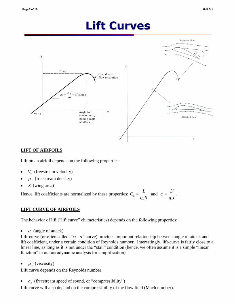
Let us look at the NACA 4412 airfoil data (Reynolds number 3106):
At 2 degrees of AOA:
cl = 0.6 cd = 0.0067 cm,c/4 = −0.08
Unit C-1Page 8 of 10
Class Example Problem C-1-2
Related Subjects . . . “NACA Airfoil Data”
A model wing of constant chord length is placed in a low
speed subsonic wind tunnel, spanning across the test
section (this is called, a quasi-2-D test). The wing has a
NACA 4412 airfoil and a chord length of 1.0 m. The test
section airspeed is 44 m/s at standard sea-level condition.
If the wing is at a 2 degrees angle of attack, determine:
(a) cl, cd, and cm,c/4
(b) the lift, the drag, and the moment about the quarter
chord (per unit span)
NACA 4412
_________________________________________________________
_________________________________________________________
_________________________________________________________
_________________________________________________________
_________________________________________________________
_________________________________________________________
_________________________________________________________
_________________________________________________________
_________________________________________________________
_________________________________________________________
_________________________________________________________
_________________________________________________________
_________________________________________________________
_________________________________________________________
_________________________________________________________
_________________________________________________________
_________________________________________________________
_________________________________________________________
_________________________________________________________
(b) The dynamic pressure is: 2 21 1(1.225)(44)
2 2q V= = = 1,185.8 N/m2
Therefore,
' (1,185.8)(1)(0.6)lL qcc= = = 711.48 N (per unit span)
' (1,185.8)(1)(0.0067)dD qcc= = = 7.945 N (per unit span)
2 2
/4 , /4' (1,185.8)(1) ( 0.08)c m cM qc c= = − = −94.86 N (per unit span)
Unit C-1Page 9 of 10
Class Example Problem C-1-2 (cont.)
Related Subjects . . . “NACA Airfoil Data”

_________________________________________________________
_________________________________________________________
_________________________________________________________
_________________________________________________________
_________________________________________________________
_________________________________________________________
_________________________________________________________
_________________________________________________________
_________________________________________________________
_________________________________________________________
_________________________________________________________
_________________________________________________________
_________________________________________________________
_________________________________________________________
_________________________________________________________
_________________________________________________________
_________________________________________________________
_________________________________________________________
_________________________________________________________
_________________________________________________________
_________________________________________________________
_________________________________________________________
Upside-down flight is equivalent to the NACA data in the range of negative angle of attack. The only
difference is that the negative angle of attack produces “downforce” (means negative lift coefficient),
while upside-down flight produces “lift” (positive lift coefficient). Thus, one can read-out the lift
coefficient from the NACA data (in the range of negative angle of attack).
(a) From NACA 4412 data (assuming the Reynolds number 3106):
At 10 = degrees => 1.34lc =
(b) If the data is read-off from “negative” angle of attack:
At 10 = − degrees => 0.64lc =
(c) Impossible.
The airfoil stalls out at about “negative” angle of attack of −12 degrees (maximum 0.8lc = )
Unit C-1Page 10 of 10
Class Example Problem C-1-3
Related Subjects . . . “NACA Airfoil Data”
Once again, can airplane fly upside-down?
To answer this question, we will use the same wind tunnel test as in Class Example
Problem C-1-2. Consider NACA 4412 airfoil.
(a) Determine the lift coefficient at an angle of attack of 10 degrees.
(b) Now imagine the same airfoil turned upside-down, but at the same 10 degrees angle
of attack as part (a). Determine its lift coefficient.
(c) At what angle of attack must the upside-down airfoil be set to generate the same lift
as that when it is right-side-up at a 10 degrees angle of attack?
NACA 4412

AE301 Aerodynamics I
UNIT C: 2-D Airfoils
ROAD MAP . . .
C-1: Aerodynamics of Airfoils 1
C-2: Aerodynamics of Airfoils 2
C-3: Panel Methods
C-4: Thin Airfoil Theory
AE301 Aerodynamics I
Unit C-2: List of Subjects
Pressure Coefficient
Obtaining Lift from CP
Compressibility Effects
Critical Mach Number
Drag-Divergence Mach Number
Supercritical Airfoil
Wave Drag

PRESSURE COEFFICIENT
Pressure coefficient (Cp) is a dimensionless quantity
−
=q
ppC
p
Convention of Cp plot: opposed vertical axis (negative up positive down)
• Cp = 1: means that the location where the velocity (V) is equal to zero (stagnation point)
Note that the “highest” positive value of pressure coefficient is: Cp = 1 (Cp cannot become more than
1: it is impossible, by definition).
• Cp = 0: means that the location where the static pressure at that point (p) becomes equal to the
freestream static pressure (p∞), commonly called: the static port location.
• Cp = negative: means that the surface pressure is lower than the freestream static pressure. The
surface of negative pressure coefficient is called “suction surface.”
• Cp = positive (but less than 1): means that the surface pressure is higher than the freestream static
pressure. The surface of positive pressure coefficient is called “pressure surface.”
CP DISTRIBUTION OVER AN AIRFOIL (WITH A SMALL POSITIVE AOA)
Upper surface: Cp at the leading edge starts from 1 (stagnation point). Cp starts to decrease (favorable
pressure gradient) very rapidly (p < p∞) and reaches the minimum pressure point. After this minimum
pressure point, Cp increases (adverse pressure gradient) toward the trailing edge.
Lower surface: Cp at the leading edge starts from 1 (stagnation point). Cp starts to decrease (favorable
pressure gradient) and then slightly increase (adverse pressure gradient) toward the trailing edge.
Unit C-2Page 1 of 11
Pressure Coefficient
Cp = 0: pressure is the same as p
Cp = 1: stagnation point
V

_________________________________________________________
_________________________________________________________
_________________________________________________________
_________________________________________________________
_________________________________________________________
_________________________________________________________
_________________________________________________________
_________________________________________________________
_________________________________________________________
_________________________________________________________
_________________________________________________________
_________________________________________________________
_________________________________________________________
_________________________________________________________
_________________________________________________________
_________________________________________________________
_________________________________________________________
_________________________________________________________
_________________________________________________________
_________________________________________________________
_________________________________________________________
_________________________________________________________
_________________________________________________________
_________________________________________________________
_________________________________________________________
At standard sea-level condition,
= 0.0023769 slug/ft3
p = 2,116.2 lb/ft2
The test section airspeed is: 70 mph = 88 ft/s
70 mph60 mph
= 102.667 ft/s
Thus, the dynamic pressure is:
2 21 1(0.0023769)(102.667)
2 2q V = = = 12.527 lb/ft2
2,100 2,116.2
12.527p
p pC
q
− −= = = 1.293−
Unit C-2Page 2 of 11
Class Example Problem C-2-1
Related Subjects . . . “Pressure Coefficient”
Consider an airfoil model mounted in a subsonic wind tunnel. The test section
airspeed is 70 mph, and the condition is the standard sea-level. If the pressure
measured at a point on the airfoil (using a static pressure tap connected to a U-tube
manometer) is 2,100 lb/ft2, what is the corresponding pressure coefficient?
Static Pressure Taps

LIFT COEFFICIENT CALCULATION FROM CP DISTRIBUTION
Lift force (per unit span) can be found by integrating Cp over the surface: TE TE
LE LE
' cos cosl uL p ds p ds = − ,
where, lp = Pressure on the lower surface
up = Pressure on the lower surface
also, cosds dx =
0 0
'
c c
l uL p dx p dx= −
Adding and subtracting p , we have: ( ) ( )0 0
'
c c
l uL p p dx p p dx = − − −
From the definition of lift coefficient:
0 0
' 1 1c c
l ul
p p p pLc dx dx
q c c q c q
− −= = − = , ,
0
1( )
c
p l p uC C dxc
−
NORMALIZED COORDINATE LOCATION
Often, it is convenient to specify the coordinate “along the chord”: x
xc
=
1
, , , ,
0 0
1( ) ( )
x cc
p l p u p l p u
x c
xC C dx C C d
c c
=
=
− = − =
1
, ,
0
( )p l p uC C dx−
Unit C-2Page 3 of 11
Obtaining Lift from CP
_________________________________________________________
_________________________________________________________
_________________________________________________________
_________________________________________________________
_________________________________________________________
_________________________________________________________
_________________________________________________________
_________________________________________________________
_________________________________________________________
_________________________________________________________
_________________________________________________________
_________________________________________________________
_________________________________________________________
_________________________________________________________
_________________________________________________________
_________________________________________________________
_________________________________________________________
_________________________________________________________
_________________________________________________________
_________________________________________________________
_________________________________________________________
_________________________________________________________
_________________________________________________________
_________________________________________________________
Unit C-2Page 4 of 11
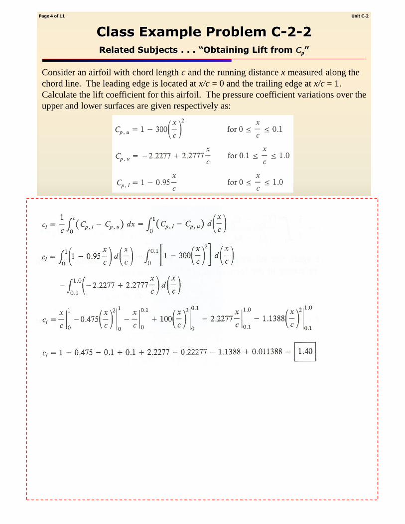
Class Example Problem C-2-2
Related Subjects . . . “Obtaining Lift from Cp”
Consider an airfoil with chord length c and the running distance x measured along the
chord line. The leading edge is located at x/c = 0 and the trailing edge at x/c = 1.
Calculate the lift coefficient for this airfoil. The pressure coefficient variations over the
upper and lower surfaces are given respectively as:

COMPRESSIBILITY CORRECTION FOR PRESSURE COEFFICIENT
As the freestream Mach number is increased (M > 0.3), the compressibility effects can no longer be
ignored. A correction for compressibility is called, the Prandtl-Glauert rule:
,0
21
p
p
CC
M
=−
• This is simply a “correction factor” and will only provide “estimated” pressure coefficient at a given
Mach number
• In order to more accurately determine pressure coefficient, one needs to apply energy equation (if it
is reasonable to assume that the flow is still isentropic and ideal gas of air).
CRITICAL MACH NUMBER
Critical Mach number (Mcr): the freestream Mach number at which sonic flow is first obtained
somewhere on the airfoil surface.
Critical pressure coefficient (Cp,cr): the specific value of Cp that corresponds to the presence of sonic
flow (M = 1).
Unit C-2Page 5 of 11
Compressibility Effects
Prandtl-Glauert Rule:

_________________________________________________________
_________________________________________________________
_________________________________________________________
_________________________________________________________
_________________________________________________________
_________________________________________________________
_________________________________________________________
_________________________________________________________
_________________________________________________________
_________________________________________________________
_________________________________________________________
_________________________________________________________
_________________________________________________________
_________________________________________________________
_________________________________________________________
_________________________________________________________
_________________________________________________________
_________________________________________________________
_________________________________________________________
EFFECTS OF AIRFOIL THCKNESS
If the airfoil is thick, the pressure at the minimum pressure point on the surface of the airfoil becomes
lower. As a result, the sonic flow begins to appear at much lower Mach number. Therefore, the critical
Mach number is lower.
EQUATION OF CRITICAL MACH NUMBER (1)
Starting from the pressure coefficient: 1p
p p p pC
q q p
−= = −
eqn. 1
Recall, the definition of dynamic pressure:
( )( )
( )2
2 21 1 1
2 2 2
Vq V p V p
p p
= = = eqn. 2
Also, recall, speed of sound is ( )2a RT p = = , and eqn. 2 becomes:
( )( ) ( )
2 22 2
2
1 1 1
2 2 2 2
V Vq V p p p M
p a
= = = = eqn. 3
Unit C-2Page 6 of 11
Critical Mach Number (1)

_________________________________________________________
_________________________________________________________
_________________________________________________________
_________________________________________________________
_________________________________________________________
_________________________________________________________
_________________________________________________________
_________________________________________________________
_________________________________________________________
_________________________________________________________
_________________________________________________________
_________________________________________________________
_________________________________________________________
_________________________________________________________
_________________________________________________________
_________________________________________________________
_________________________________________________________
_________________________________________________________
_________________________________________________________
_________________________________________________________
_________________________________________________________
_________________________________________________________
_________________________________________________________
_________________________________________________________
EQUATION OF CRITICAL MACH NUMBER (2)
Recall, for isentropic flow (between freestream and stagnation point):
( )1
20 11
2
pM
p
−−
= +
eqn. 4
Applying eqn. 4 between freestream and stagnation point:
( )1
20 11
2
pM
p
−
− = +
eqn. 5
Combining eqns. 4 & 5 yields: ( )
( )
( )1
2
0
20
11 1
21
1 12
Mpp p
p p pM
−
+ −
= = + −
eqn. 6
Now, substituting eqn. 6 into eqn. 1:
( )
( )
( )
( )
( )
( )1 1
2 2
22 2 2
1 11 1 1 1
22 21 1 11 1 1
1 1 1 12 2 2
p
M Mp pp
Cq p M
p M M M
− −
+ − + −
= − = − = − + − + −
Cp = Cp,cr, where M = 1, therefore the Cp at critical Mach number is:
( )( )1
2
, 2
2 121
1p cr
MC
M
−
+ − = −
+
Unit C-2Page 7 of 11
Critical Mach Number (2)

DRAG DIVERGENCE MACH NUMBER
Drag divergence Mach number: the freestream Mach number at which drag coefficient begins to
increase rapidly.
Mcr < Mdrag divergence < 1.0
Drag divergence is based mainly on the formation of strong normal shock wave at the minimum
pressure point on the upper surface of the airfoil and associated flow separation behind the shock wave,
called the “shock-induced” flow separation.
• Due to the drag divergence, the early attempts of supersonic flight (NASA / Bell X-1) faced
difficulties of achieving the successful supersonic flight: this is commonly known as a “SONIC
BARRIER.”
Unit C-2Page 8 of 11
Drag-Divergence Mach Number

SUPERCRITICAL AIRFOIL
A supercritical (SC) airfoil (NASA-SC or NACA 8-series) is an airfoil designed, primarily, to delay the
onset of wave drag in the transonic speed range. The supercritical airfoil was created in the 1960s, by
NASA scientist Richard Whitcomb.
While the design was initially developed as part of the supersonic transport (SST) project at NASA, it
has since been mainly applied to increase the fuel efficiency of many high subsonic aircraft.
Supercritical airfoils have three main benefits:
• Higher (or “delayed”) critical Mach number,
• Develop shock waves further aft than traditional airfoils, and thus,
• Greatly reduce shock-induced boundary layer separation.
NASA-SC airfoil is relatively “thick” airfoil and not suitable for supersonic flight. The design purpose
is to delay formation of “shock-induced flow separation” to avoid drag divergence at the high-end of
transonic flight.
Boeing (MD) C-17 Globemaster III (US Patent
No: 4,858,853, McDonnell Douglas Corporation,
1987)
Unit C-2Page 9 of 11
Supercritical Airfoil
NASA-SC
Characteristics of NASA-SC Airfoil:• Flattened upper surface,• Highly cambered (curved) aft section, and• Greater leading edge radius as compared to traditional airfoils

WAVE DRAG
Wave drag is the pressure drag due to the formation of shock waves. At supersonic flight, the entire
vehicle is placed “behind” the shockwave. Under this condition, the flow behind the shockwave is not
the same condition of freestream: it is much higher pressure, density, and temperature.
Wave drag is usually the order of magnitude higher than other drag components (such as skin friction &
pressure drags). Super-cruising (cruising at supersonic) is technically very challenging, due to the
massive increase of drag (due to the formation of shock waves: wave drag), usually requires higher
thrust to compensate the higher drag for supersonic cruising.
AERODYNAMIC COEFFICIENTS AT SUPERSONIC FLIGHT
Lift and drag at supersonic flight is mainly dependent upon Mach number (as well as the angle of
attack). For a thin supersonic airfoil (close to a flat plate), the lift and wave drag coefficients can be
estimated as:
2
4 or
1l Lc C
M
=−
2
, ,2
4 or
1d w D wc C
M
=−
Unit C-2Page 10 of 11
Wave Drag
2
, ,2
4 or
1d w D wc C
M
=−
2
4 or
1l Lc C
M
=−

_________________________________________________________
_________________________________________________________
_________________________________________________________
_________________________________________________________
_________________________________________________________
_________________________________________________________
_________________________________________________________
_________________________________________________________
_________________________________________________________
_________________________________________________________
_________________________________________________________
_________________________________________________________
_________________________________________________________
_________________________________________________________
_________________________________________________________
_________________________________________________________
_________________________________________________________
_________________________________________________________
_________________________________________________________
_________________________________________________________
_________________________________________________________
_________________________________________________________
_________________________________________________________
_________________________________________________________
_________________________________________________________
Lift and wave drag coefficients can be calculated as:
= 5 degrees = 5(/180) = 0.087266 radians
2 2
4 4(0.087266)
1 (3) 1lc
M
= =− −
= 0.1234
2 2
,2 2
4 4(0.087266)
1 (3) 1d wc
M
= =− −
= 0.01077
At 22,000 ft:
= 0.0011836 slug/ft3
a = 1,028.6 ft/s => M = 3 means that V = (1,028.6)(3) = 3,085.8 ft/s
2 21 1(0.0011836)(3,085.8)
2 2q V = = = 5,635.215 lb/ft2
Hence, lift and wave drag (per unit span) are:
' (5,635.215)(10)(0.1234)lL q cc= = = 6,953.85 lb
,' (5,635.215)(10)(0.01077)w d wD q cc= = = 606.91 lb
Unit C-2Page 11 of 11
Class Example Problem C-2-3
Related Subjects . . . “Wave Drag”
Consider a thin supersonic airfoil with chord length c = 10 ft in a Mach 3 freestream at
an altitude of 22,000 ft. The airfoil is at an angle of attack of 5 degrees. Calculate the
lift & wave drag coefficients and the lift & wave drag per unit span.
Figure: X-43 Hyper X Prototype(NASA Ames Research Center)

AE301 Aerodynamics I
UNIT C: 2-D Airfoils
ROAD MAP . . .
C-1: Aerodynamics of Airfoils 1
C-2: Aerodynamics of Airfoils 2
C-3: Panel Methods
C-4: Thin Airfoil Theory
AE301 Aerodynamics I
Unit C-3: List of Subjects
Problem Solutions? How?
Source Panel Method
Vortex Panel Method
This is a tutorial (self-study) material for the COURSE PROJECT
• Not covered in class as a standard lecture of AE301
• Online lecture (YouTube) Available

PANEL METHODS / THIN AIRFOIL THEORY: PURE THEORETICAL SCHEMES
Panel methods and thin airfoil theory are built upon potential flow analysis. In other words, these are
pure theoretical schemes. Similar to the unit B-3, as we deal with the pure theory, one must be very
carefully recognize (and keep track of) the followings:
(1) What are the assumptions made to simplify the equation?
• Steady-state?
• Inviscid?
• No body forces?
• Incompressible?
• Irrotational?
(2) Because of the assumptions made, how your theoretical solution different (or apart) from the actual
(or real) flow field phenomena?
Unit CUnit C--33Page Page 11 of 12of 12
Problem Solutions? How?Problem Solutions? How?

SOURCE PANEL METHOD
A source sheet can be defined as infinite number of line sources (side by side) where the strength of
each line source is infinitesimally small.
Source strength per unit length can be defined as: ( )s = .
Consider an arbitrary point ( , )P x y . . . a small section of the source sheet of strength ds induces an
infinitesimally small velocity potential d :
ln2
dsd r
=
Thus, the complete velocity potential at point P induced by the entire source sheet is:
( , ) ln2
b
a
dsx y r
=
Unit CUnit C--33Page Page 22 of 12of 12
Source Panel Method (1)Source Panel Method (1)

Let us approximate the source sheet by a series of straight panels, moreover, let the source strength per
unit length be constant over a given panel.
For the total number of n panels, the source strengths per unit length for each panel can be represented
by: 1 2 3, , , , ,j n
Then, solve: , 1, 2,3 ,j j n = such that the body surface becomes a streamline of the flow: means that
the boundary condition is imposed numerically by j ’s such that the normal component of the flow
velocity is zero at the midpoint of each panel (called, the “control point”).
Again, consider a point P (x,y) in the flow field, and let pjr be the distance from any point on the jth
panel to P.
The velocity potential induced at P due to the jth panel is:
ln2
j
j pj j
j
r ds
=
Unit CUnit C--33Page Page 33 of 12of 12
Source Panel Method (2)Source Panel Method (2)

The potential at P due to all panels is:
( )1 1
ln2
n nj
j pj j
j j j
P r ds
= =
= =
where, the distance 2 2( ) ( )pj j jr x x y y= − + −
Next, let us put P at the control point of the jth panel ( , )i iP x y :
( )1
, ln2
nj
i i ij j
j j
x y r ds
=
= 2 2( ) ( )ij i j i jr x x y y= − + −
This is the contribution of all panels to the potential at the control point of the ith panel.
The free stream component normal to the panel is:
,ˆ cosn i iV V n V = =
The normal component of velocity induced at ( , )i ix y by a panel is:
( , )n i i
i
V x yn
=
Unit CUnit C--33Page Page 44 of 12of 12
Source Panel Method (3)Source Panel Method (3)

Combining this with the potential ( , )i ix y , which is contribution of all the panels to the potential at the
control point of the ith panel:
( )1
( 1)
ln2 2
nji
n ij j
j ijj
V r dsn
=
= +
Applying the boundary condition, , 0n nV V + = , yields:
( )1
( 1)
ln cos 02
ni
ij j i
j ijj
r ds Vn
=
+ + =
Let: , ,(ln )i j i j j
ij
I r dsn
=
=> ( )
,
1 1
cos 02 2
nji
i j i
j j
I V
=
+ + =
This is a linear algebraic equation with n unknowns ( 1 2 3, , , , ,j n ) => these unknowns can
be solved (n equations with n unknowns)
Once ’s are all solved ( , 1,2,3 ,i i n = ) . . .
The component of free stream velocity tangent to the surface is:
, sins iV V =
The tangential velocity sV at the control point of the ith panel induced by all the panels is:
( )1
ln2
ni
s ij j
j j
V r dss s
=
= =
The total surface velocity at the ith control point iV is the sum of the contribution from the free stream
and from the source panels:
( ),
1
sin ln2
ni
i s s i ij j
j j
V V V V r dss
=
= + = +
Finally, the pressure coefficient at the ith panel can be given as: 2
, 1 ( )p i iC V V= −
Unit CUnit C--33Page Page 55 of 12of 12
Source Panel Method (4)Source Panel Method (4)

Source panel code has two fundamental problems:
• Source panel does not simulate circulation. Therefore, the source panel code’s application is
inherently limited to a nonlifting flow around a body only.
• Source panel cannot enforce the Kutta condition at the trailing edge. Therefore, the stagnation
point is formed at an arbitrary location as the angle of attack is increased, and this causes the
nonphysical solutions.
Unit CUnit C--33Page Page 66 of 12of 12
Class Example Problem CClass Example Problem C--33--11
Related Subjects . . . Related Subjects . . . ““Source Panel MethodSource Panel Method””
There is a “theoretical” airfoil, called a “Joukowski” airfoil. The shape of this airfoil
can be obtained from a circle by a mathematical transformation between two domains.
Since this airfoil is a theoretically derived shape, the surface pressure coefficient
distribution (Cp) can also be obtained theoretically. Using source panel method,
calculate the pressure coefficient distribution (Cp) of symmetic Joukowski airfoil at
AOA = 0. Compare the theoretical distribution of Cp (Joukowski airfoil: known
values) against Cp computed by the source panel method.
Symmetric Joukowski Airfoil

VORTEX SHEET
A vortex filament can be defined as a straight line perpendicular to the page, going through point O
(extend to infinity both sides).
A vortex sheet can be defined as infinite number of vortex filaments side by side, with the strength of
each filament is infinitesimally small.
Consider an arbitrary point P (x, z). The small section of vortex sheet of strength ds induces a small
velocity potential and velocity dV :
2
dsd
= − and
2
dsdV
r
= −
The velocity potential at P due to entire vortex sheet from a to b is, therefore:
1( , )
2
b
a
x z ds
= − where, the circulation is:
b
a
ds =
Unit CUnit C--33Page Page 77 of 12of 12
Vortex Panel Method (1)Vortex Panel Method (1)

Consider a dashed path enclosing a vortex sheet of strength ds :
2 1 1 2 1 2 1 2( ) ( ) ( )C
v dn u ds v dn u ds u u ds v v dn = − = − − − + = − + − V ds
Let the top and bottom of the dashed line approach the vortex sheet:
0dn → , and 1 2u u = −
Important conclusion: the local jump in tangential velocity across the vortex sheet is equal to the local
sheet strength. This is the fundamental concept of thin airfoil theory.
The vortex panel method is built upon the idea that, if we replace the 2-D airfoil shape by a vortex sheet,
it is possible to obtain the lift using the Kutta-Joukowski theorem.
Thin airfoil theory and vortex panel method are built upon the same fundamental models of vortex sheet.
• If airfoil is thin => thin airfoil theory
• If airfoil is not thin => vortex panel method
Unit CUnit C--33Page Page 88 of 12of 12
Vortex Panel Method (2)Vortex Panel Method (2)
1 2u u = −ds =

VORTEX PANEL METHOD
Very similar approach (as discussed in source panel method).
A series of vortex sheets approximates the body of arbitrary shape (vortex panels):
Total number of n panels with the vortex strengths per unit length of: 1 2 3, , , , ,j n
At the control points, the normal component of the velocity is zero:
, 0n nV V + =
1
cos 02
nj ij
i j
j ij
V dsn
=
− =
or
1
cos 02
nj
i ij
j
V I
=
− =
Note that the Kutta condition can be applied precisely at the trailing edge and is given by (TE) 0 = ,
means at trailing edge: 1i i −= −
This Kutta condition forces the flow field to have a proper stagnation point at (or near) the trailing edge
of the flow field.
Unit CUnit C--33Page Page 99 of 12of 12
Vortex Panel Method (3)Vortex Panel Method (3)

Once the unknown vortex strength, 1 2 3, , , , ,j n , are obtained, the total circulation for the given
flow field can be calculated as:
1
n
j j
j
s=
=
Therefore, the lift per unit span is (from the Kutta-Joukowski theorem):
1
'n
j j
j
L V s
=
=
Unit CUnit C--33Page Page 1010 of 12of 12
Vortex Panel Method (4)Vortex Panel Method (4)

VARIETY OF SOURCE / VORTEX PANEL METHOD SCHEMES
• 1st order vortex panel method: the strength of vortex panel is constant for a given panel.
• 2nd order vortex panel method: the strength of vortex panel varies linearly over a given panel.
• Combination of source + vortex panels: use source panel to simulate the airfoil thickness, use vortex
panel to introduce circulation (lift).
Unit CUnit C--33Page Page 1111 of 12of 12
Vortex Panel Method (5)Vortex Panel Method (5)

There are a few important restrictions of using Vortex Panel Java Applet
• Airfoil coordinate data must be arranged that:
Trailing Edge (1,0) => Lower Surface Data => Leading Edge (0,0) => Trailing Edge
• Too much panels clustered near the trailing edge will make it difficult to properly apply Kutta
condition: you may want to manually remove some panels.
• Total number of panels should be in the range of 30 to 100. Using too many panels will slow down
computations and will not necessarily improve the accuracy.
Unit CUnit C--33Page Page 1212 of 12of 12
Class Example Problem CClass Example Problem C--33--22
Related Subjects . . . Related Subjects . . . ““Vortex Panel MethodVortex Panel Method””
Using Virginia Tech vortex panel method (Java Applet), determine the lift coefficient
of NACA 0009 airfoil over a range of angles of attack from 0 to 16 degrees. Plot a lift
curve (cl v.s. ) and compare it against NACA airfoil data.
http://www.engapplets.vt.edu/
Lift Coefficient v.s. AOA
0
0.2
0.4
0.6
0.8
1
1.2
1.4
1.6
1.8
2
0 2 4 6 8 10 12 14 16
AOA (degrees)
Se
cti
on
Lif
t C
oe
ffic
ien
t
Vortex Panel Method NACA 0009 Data
AOA
(degrees) Vortex Panel Method NACA 0009 Data
0 0 0
1 0.118183
2 0.23633 0.2
3 0.354404
4 0.472371 0.4
5 0.590194
6 0.707837 0.6
7 0.825265
8 0.942441 0.85
9 1.05933
10 1.175896 1.08
11 1.292105
12 1.407919 1.26
13 1.523305
14 1.638227 1.3
15 1.752649
16 1.866538 1.14
Lift Coefficient

AE301 Aerodynamics I
UNIT C: 2-D Airfoils
ROAD MAP . . .
C-1: Aerodynamics of Airfoils 1
C-2: Aerodynamics of Airfoils 2
C-3: Panel Methods
C-4: Thin Airfoil Theory
AE301 Aerodynamics I
Unit C-4: List of Subjects
Thin Airfoil Approximation
Thin Airfoil Theory
Symmetric Thin Airfoil
Cambered Thin Airfoil
Real Flow over an Airfoil
This is for your REFERENCE purposes (self-study) only
• Useful for your future needs (aero-track courses)
• Not covered as a standard material in AE301
• Not included in any exam
• Online lecture (YouTube) Available
•

THIN AIRFOIL APPROXIMATION
If the airfoil is thin, a single vortex sheet can be used to approximate a thin airfoil by replacing it along
the camber line: thin airfoil theory.
PRANDTL’S CLASSICAL THIN AIRFOIL THEORY
The classical Prandtl’s thin airfoil theory is covered here:
• Rather than modeling the mean camber line by vortex sheet, the chord line (the straight line
connecting between leading edge and trailing edge) is represented by a vortex sheet as a function of
straight horizontal coordinate system (x): the vortex sheet is placed on the chord line: ( )x =
• The camber line is forced to be a streamline, and is calculated to satisfy this condition as well as
Kutta condition: ( ) 0c =
• For the camber line to be a streamline, the normal component of freestream is going to be cancelled
by the downwash generated by the vortex sheet (everywhere along the mean camber line);
mathematically: , '( ) 0nV w s + =
Unit C-4Page 1 of 10
Thin Airfoil Approximation

At any point P on the camber line, where the slope of the camber line is dz dx , 1
, sin[ tan ( )]nV V dz dx −
= + −
For a thin airfoil, both and 1tan ( )dz dx− − are small values, and for a small angle: sin tan ,
so , [ ]nV V dz dx = −
The velocity dw at location x induced by the small elemental vortex d at location is given by:
( )
2 ( )
ddw
x
= −
−
Thus, the velocity ( )w x induced at location x by all the elemental vortices along the chord line can be
obtained by integrating dw from the leading edge ( 0 = ) to the trailing edge ( c = ) as:
0
( )( )
2 ( )
cd
w xx
= −
−
Unit C-4Page 2 of 10
Thin Airfoil Theory (1)

Recall, for the camber line to be streamline:
, '( ) 0nV w s + = , where '( ) ( )w s w x for thin airfoil, so
0
( )0
2 ( )
cdz d
Vdx x
− − =
−
0
1 ( )
2
cd dz
Vx dx
= −
−
This is the governing equation of thin airfoil theory.
Unit C-4Page 3 of 10
Thin Airfoil Theory (2)

SYMMETRIC THIN AIRFOIL SOLUTIONS (1)
For symmetric airfoil: 0dz dx = , therefore:
0
1 ( )
2
cd
Vx
=
−
Transformation from to : (1 cos )2
c = − , sin
2
cd d =
Transformation from x to 0 : 0(1 cos )2
cx = −
00
1 ( )sin
2 cos cos
dV
=−
The mathematical solution to this equation is:
(1 cos )( ) 2
sinV
+=
Unit C-4Page 4 of 10
Symmetric Thin Airfoil (1)

SYMMETRIC THIN AIRFOIL SOLUTIONS (2)
The total circulation around the airfoil is: 0 0
( ) ( )sin2
cc
d d
= =
Solution of the thin airfoil theory is: 0
(1 cos )cV d cV
= + =
LIFT AND MOMENT COEFFICIENTS
From the Kutta-Joukowski theorem: 2'L V c V = =
The lift coefficient: 2
2
'
1
2
l
c VLc
q cV c
= = = 2
Moment at leading edge: 0 0
' ( ) ( )
c c
LEM dL V d = − = −
=> through transformation and integration: 2'
2LEM q c
= −
The moment coefficient: LE, le 2
'
2m
Mc
q c
= = − =4
lc−
The moment coefficient at quarter chord point (recall, from Unit A-5):
, 4 , le4 4 4
l l lm c m
c c cc c= + = − + = 0
CENTER OF PRESSURE AND AERODYNAMICS CENTER LOCATIONS
The location of center of pressure is: , 4
cp
1 1 0
4 4 2
m c
l
cx
c = − = − =
1
4
The location of aerodynamic center is: 0ac
0
1 0 1
4 2 4
mx
a = − + = − + =
1
4
• For a symmetric thin airfoil, the quarter-chord point is both the center of pressure and the
aerodynamic center.
Unit C-4Page 5 of 10
Symmetric Thin Airfoil (2)

Using the thin airfoil theory:
At 4 degrees AOA: 4 degrees = 4( /180) = 0.06981 rad
(a) 2 2 (0.06981)lc = = = 0.4386
(b) , /4m cc = 0
Unit C-4Page 6 of 10
Class Example Problem C-4-1
Related Subjects . . . “Thin Airfoil Theory”
Consider a symmetric thin airfoil (such as NACA 0006) at 4 degrees angle of attack.
Using the thin airfoil theory, calculate the followings and compare them against NACA
airfoil data:
(a) The lift coefficient
(b) The moment coefficient at the quarter chord

From NACA 0006 airfoil data, at 4 degrees AOA: 4 degrees:
(a) lc = 0.4
(b) , / 4m cc = 0
Unit C-4Page 7 of 10
Class Example Problem C-4-1 (cont.)
Related Subjects . . . “Thin Airfoil Theory”
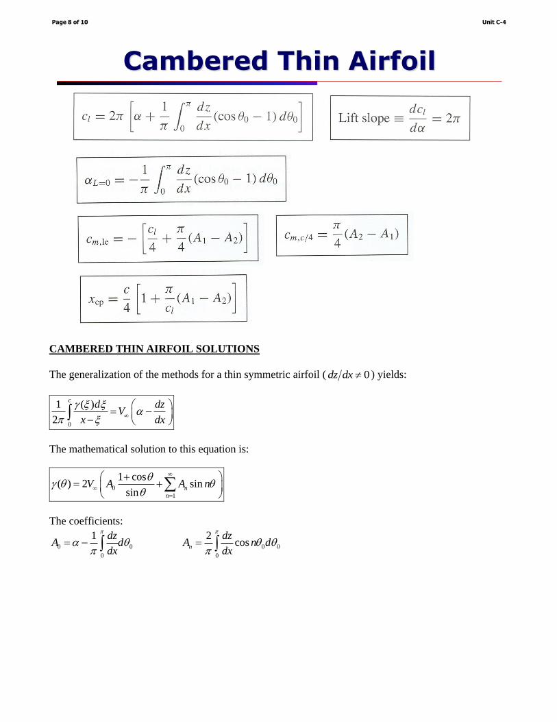
CAMBERED THIN AIRFOIL SOLUTIONS
The generalization of the methods for a thin symmetric airfoil ( 0dz dx ) yields:
0
1 ( )
2
cd dz
Vx dx
= −
−
The mathematical solution to this equation is:
0
1
1 cos( ) 2 sin
sinn
n
V A A n
=
+ = +
The coefficients:
0 0
0
1 dzA d
dx
= − 0 0
0
2cosn
dzA n d
dx
=
Unit C-4Page 8 of 10
Cambered Thin Airfoil

LEADING EDGE STALL
Example: NACA 4412
Characteristics of relatively thin airfoils with thickness ratios between 10 and 16 percent of the chord
length.
• Post-stall characteristics: rapid loss of the lift
Unit C-4Page 9 of 10
Real Flow over an Airfoil (1)
NACA 4412

EFFECTS OF AIRFOIL THICKNESS ON STALL
Thin airfoil: thin airfoil is desired for high-speed applications (from high transonic to supersonic), in
order to minimize profile and wave drags.
Thick airfoil: thick airfoil is desired for low-speed applications (low subsonic), due to the favorable stall
characteristics.
Unit C-4Page 10 of 10
Real Flow over an Airfoil (2)
NACA 4421