4 D - 1: Unit D - 0: List of Subjects
34
ES206 Fluid Mechanics UNIT D: Flow Field Analysis ROAD MAP . . . D-0: Reynolds Transport Theorem D-1: Conservation of Mass D-2: Conservation of Momentum D-3: Conservation of Energy Unit D-0: List of Subjects Eulerian and Lagrangian Streamline, Streakline, and Pathline System v.s. Control Volume Reynolds Transport Theorem Types of Control Volume
Transcript of 4 D - 1: Unit D - 0: List of Subjects
ES206 Fluid Mechanics
UNIT D: Flow Field Analysis
ROAD MAP . . .
D-0: Reynolds Transport Theorem
D-1: Conservation of Mass
D-2: Conservation of Momentum
D-3: Conservation of Energy
ES206 Fluid Mechanics
Unit D-0: List of Subjects
Eulerian and Lagrangian
Streamline, Streakline, and Pathline
System v.s. Control Volume
Reynolds Transport Theorem
Types of Control Volume

_________________________________________________________
_________________________________________________________
_________________________________________________________
_________________________________________________________
_________________________________________________________
_________________________________________________________
_________________________________________________________
_________________________________________________________
_________________________________________________________
_________________________________________________________
Eulerian and Lagrangian: 2 Different Approaches in Flow Field Analysis
Eulerian method = “INTEGRATION” of properties into the “FIELD” of flow
(this field is often called, the CONTROL VOLUME).
Lagrangian method = “DIFFERENTIATION” of properties onto each
“PARTICLE” of flow (the collection of all particles of flow is often called, the
SYSTEM).
Unit D-0Page 1 of 12
Eulerian and Lagrangian
UNIT DUNIT D--11SLIDE SLIDE 77
EulerianEulerian and and LagrangianLagrangian (1)(1)
➢ There are two general approaches in analyzing fluid mechanics problems: Eulerian and Lagrangian methods
➢ Eulerian method: uses the field representation concept
➢ Lagrangian method: involves tracing individual fluid particles as they move and determining how the fluid properties associated with these particles change as a function of time – the fluid particles are “tagged” or identified, and their properties determined as they move
_________________________________________________________
_________________________________________________________
_________________________________________________________
_________________________________________________________
_________________________________________________________
_________________________________________________________
_________________________________________________________
_________________________________________________________
_________________________________________________________
_________________________________________________________
_________________________________________________________
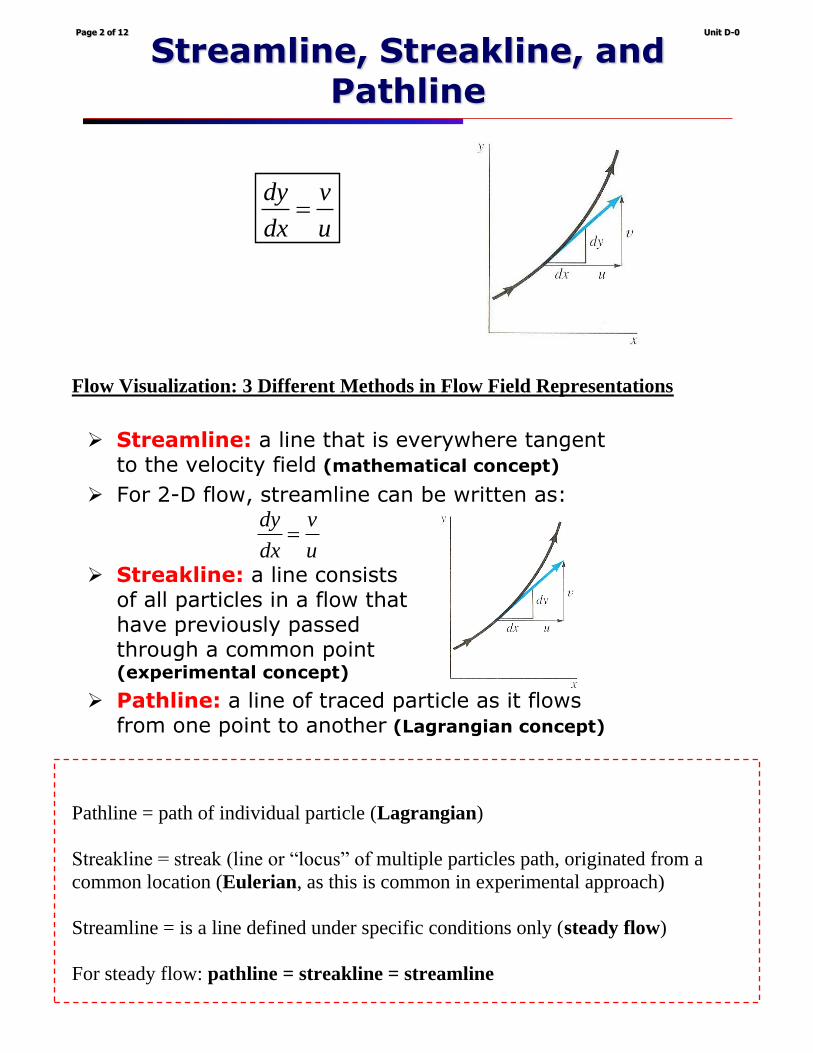
Flow Visualization: 3 Different Methods in Flow Field Representations
Pathline = path of individual particle (Lagrangian)
Streakline = streak (line or “locus” of multiple particles path, originated from a
common location (Eulerian, as this is common in experimental approach)
Streamline = is a line defined under specific conditions only (steady flow)
For steady flow: pathline = streakline = streamline
Unit D-0Page 2 of 12
Streamline, Streakline, and Pathline
u
v
dx
dy=
UNIT DUNIT D--11SLIDE SLIDE 1515
u
v
dx
dy=
➢ Streamline: a line that is everywhere tangent to the velocity field (mathematical concept)
➢ For 2-D flow, streamline can be written as:
➢ Streakline: a line consists of all particles in a flow that have previously passed through a common point (experimental concept)
➢ Pathline: a line of traced particle as it flows from one point to another (Lagrangian concept)
Streamline, Streamline, StreaklineStreakline, and , and
PathlinePathline
Textbook (Munson, Young, and Okiishi), page 156

Unit D-0Page 3 of 12
System v.s. Control Volume (1)
System = Lagrangian ApproachControl Volume = Eulerian Approach
mbB =
UNIT DUNIT D--33SLIDE SLIDE 11
System System v.sv.s. Control Volume. Control Volume (1)(1)
➢ A fluid is a type of matter that is relatively free to move and interact with its surroundings
➢ System approach: a system is a collection of matter of fixed identity (always the same atoms or fluid particles) , which may move, flow, and interact with its surroundings (Lagrangianconcept)
➢ Control volume approach: a control volume is a volume in space (a geometric entity, independent of mass) through which fluid may flow (Eulerian concept)
UNIT DUNIT D--33SLIDE SLIDE 22
System System v.sv.s. Control Volume. Control Volume (2)(2)
➢ In many ways, the relationship between asystem and a control volume is similar to the relationship between the Lagrangian and Eulerian flow description
➢ All of the laws governing the motion of a fluid are stated in their basic form in terms of a system approach (not a control volume approach)
➢ “The mass of a “system” remains constant”
➢ The time rate of change of momentum of a “system” is equal to the sum of all the forces acting on the system
UNIT DUNIT D--33SLIDE SLIDE 33
System System v.sv.s. Control Volume. Control Volume (3)(3)
➢ The Reynolds transport theorem: the governing laws of fluid motion
➢ Let B represent any fluid parameter (velocity, acceleration, mass, momentum, etc.) and brepresent the amount of that parameter per unit mass, then:
mbB =
ExtensiveProperty
Mass of the portionof fluid of interest
IntensiveProperty
_________________________________________________________
_________________________________________________________
_________________________________________________________
_________________________________________________________
_________________________________________________________
_________________________________________________________
_________________________________________________________
_________________________________________________________
_________________________________________________________
_________________________________________________________
_________________________________________________________
_________________________________________________________
_________________________________________________________
_________________________________________________________
_________________________________________________________
_________________________________________________________
_________________________________________________________
_________________________________________________________
_________________________________________________________
_________________________________________________________
_________________________________________________________
_________________________________________________________
_________________________________________________________
_________________________________________________________
_________________________________________________________
_________________________________________________________
_________________________________________________________
_________________________________________________________
_________________________________________________________
_________________________________________________________
_________________________________________________________
_________________________________________________________
_________________________________________________________
_________________________________________________________
_________________________________________________________
_________________________________________________________
_________________________________________________________
_________________________________________________________
_________________________________________________________
_________________________________________________________
_________________________________________________________
_________________________________________________________
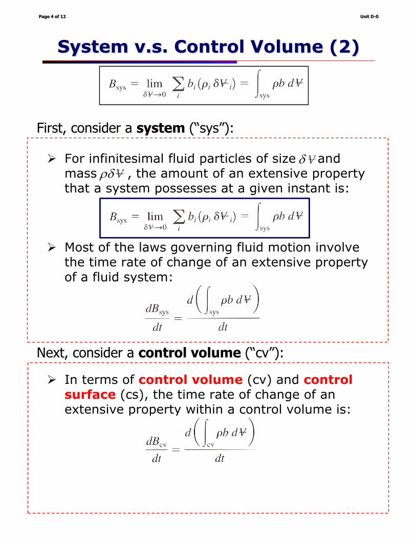
First, consider a system (“sys”):
Next, consider a control volume (“cv”):
Unit D-0Page 4 of 12
System v.s. Control Volume (2)
UNIT DUNIT D--33SLIDE SLIDE 44
System System v.sv.s. Control Volume. Control Volume (4)(4)
➢ For infinitesimal fluid particles of size and mass , the amount of an extensive property that a system possesses at a given instant is:
➢ Most of the laws governing fluid motion involve the time rate of change of an extensive property of a fluid system:
UNIT DUNIT D--33SLIDE SLIDE 55
System System v.sv.s. Control Volume. Control Volume (5)(5)
➢ In terms of control volume (cv) and control surface (cs), the time rate of change of an extensive property within a control volume is:
➢ Differences between control volume and system concepts are subtle, but very important
➢ Control volume: a volume in space (in most cases stationary, although if it moves it need NOT move with the system
➢ System: an identifiable collection of mass that moves with the fluid

_________________________________________________________
_________________________________________________________
_________________________________________________________
_________________________________________________________
_________________________________________________________
_________________________________________________________
_________________________________________________________
_________________________________________________________
_________________________________________________________
_________________________________________________________
_________________________________________________________
_________________________________________________________
_________________________________________________________
_________________________________________________________
_________________________________________________________
_________________________________________________________
_________________________________________________________
_________________________________________________________
_________________________________________________________
_________________________________________________________
_________________________________________________________
_________________________________________________________
_________________________________________________________
_________________________________________________________
_________________________________________________________
_________________________________________________________
Let B m= (mass as an extensive property) and 1b =
(1) syssys sys
d dVdB dm
dt dt dt
= =
This represents the “time rate of change” of system mass (“system mass” here is
essentially the mass of all fire extinguisher fluid particles).
As the release valve is open ( 0t ), the system (fluid particles) simply move from one
place (inside of the tank) to another (outside of the tank). Therefore, the system mass
remains constant, or:
sys0
dB
dt=
(2) cvcv cv
d dVdB dm
dt dt dt
= =
This represents the “time rate of change” of control volume mass (“control volume mass”
here is essentially the mass contained within the fixed control volume: means inside of
the fire extinguisher).
As the release valve is opened ( 0t ), the mass within the fixed control volume (inside of
the fire extinguisher) decreases. Therefore:
cv 0dB
dt
Unit D-0Page 5 of 12
EXAMPLE 4.7Textbook (Munson, Young, and Okiishi), page 171
Time Rate of Change for a System and a Control Volume

_________________________________________________________
_________________________________________________________
_________________________________________________________
_________________________________________________________
_________________________________________________________
_________________________________________________________
_________________________________________________________
_________________________________________________________
_________________________________________________________
_________________________________________________________
_________________________________________________________
_________________________________________________________
_________________________________________________________
_________________________________________________________
_________________________________________________________
_________________________________________________________
_________________________________________________________
_________________________________________________________
_________________________________________________________
_________________________________________________________
Unit D-0Page 6 of 12
Reynolds Transport Theorem (1)
UNIT DUNIT D--33SLIDE SLIDE 88
➢ The system at time : SYS = CV
➢ The system at time : SYS = CV − I + II
Reynolds Transport TheoremReynolds Transport Theorem (1)(1)
t
tt +
)()( cvsys tBtB =
)()()()( IIIcvsys ttBttBttBttB +++−+=+
Textbook (Munson, Young, and Okiishi), page 172
UNIT DUNIT D--33SLIDE SLIDE 99
Reynolds Transport TheoremReynolds Transport Theorem (2)(2)
➢ The change in the amount of B in the system in the time interval is given by:t
t
ttB
t
ttB
t
tBttB
t
tBttBttBttB
t
tBttB
t
B
)()()()(
)()()()(
)()(
IIIcvcv
sysIIIcv
syssyssys
++
+−
−+=
−+++−+=
−+=
)()( cvsys tBtB =
_________________________________________________________
_________________________________________________________
_________________________________________________________
_________________________________________________________
_________________________________________________________
_________________________________________________________
_________________________________________________________
_________________________________________________________
_________________________________________________________
_________________________________________________________
_________________________________________________________
_________________________________________________________
_________________________________________________________
_________________________________________________________
_________________________________________________________
_________________________________________________________
_________________________________________________________
_________________________________________________________
_________________________________________________________
_________________________________________________________
_________________________________________________________
_________________________________________________________
_________________________________________________________
_________________________________________________________
_________________________________________________________
_________________________________________________________
_________________________________________________________
_________________________________________________________
_________________________________________________________
_________________________________________________________
_________________________________________________________
_________________________________________________________
_________________________________________________________
_________________________________________________________
_________________________________________________________
_________________________________________________________
_________________________________________________________
_________________________________________________________
_________________________________________________________
_________________________________________________________
_________________________________________________________
_________________________________________________________
_________________________________________________________
Unit D-0Page 7 of 12
Reynolds Transport Theorem (2)
UNIT DUNIT D--33SLIDE SLIDE 1010
Reynolds Transport TheoremReynolds Transport Theorem (3)(3)
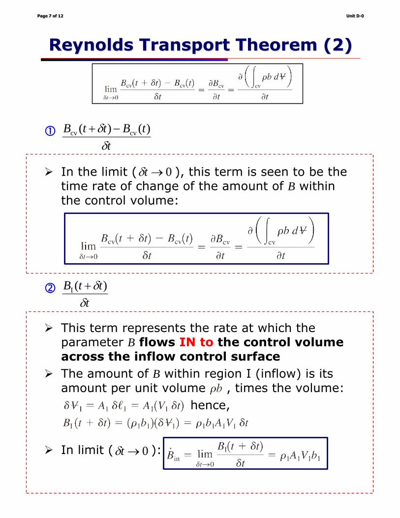
➢ In the limit ( ), this term is seen to be the time rate of change of the amount of B within the control volume:
t
tBttB
)()( cvcv −+
0→t
UNIT DUNIT D--33SLIDE SLIDE 1010
Reynolds Transport TheoremReynolds Transport Theorem (3)(3)
➢ In the limit ( ), this term is seen to be the time rate of change of the amount of B within the control volume:
t
tBttB
)()( cvcv −+
0→t
UNIT DUNIT D--33SLIDE SLIDE 1111
➢ This term represents the rate at which the parameter B flows IN to the control volumeacross the inflow control surface
➢ The amount of B within region I (inflow) is its amount per unit volume , times the volume:
hence,
➢ In limit ( ):
Reynolds Transport TheoremReynolds Transport Theorem (4)(4)
t
ttB
)(I +
0→t

_________________________________________________________
_________________________________________________________
_________________________________________________________
_________________________________________________________
_________________________________________________________
_________________________________________________________
_________________________________________________________
_________________________________________________________
_________________________________________________________
_________________________________________________________
_________________________________________________________
_________________________________________________________
_________________________________________________________
_________________________________________________________
_________________________________________________________
_________________________________________________________
_________________________________________________________
_________________________________________________________
_________________________________________________________
_________________________________________________________
_________________________________________________________
_________________________________________________________
_________________________________________________________
_________________________________________________________
_________________________________________________________
_________________________________________________________
_________________________________________________________
_________________________________________________________
Reynolds Transport Theorem (for a flow of a variable cross section pipe)
Taking the limit of the LHS of the equation:
sys sys
0lim
t
B DB
t Dt
→
=
(substantial, or total, change of system property)
Taking the limit of the RHS of the equation:
( ) ( )cv cv cv
0lim
t
B t t B t B
t t
→
+ − =
(change of property within the control volume)
& ( )I or II
in out0
lim or t
B t tB B
t
→
+ =
(property’s flux, in or out)
sys cvout in
DB BB B
Dt t
= + −
(Reynolds Transport Theorem)
Unit D-0Page 8 of 12
Reynolds Transport Theorem (3)UNIT DUNIT D--33SLIDE SLIDE 1212
➢ This term represents the rate at which the parameter B flows OUT of the control volumeacross the outflow control surface
➢ The amount of B within region II (outflow) is its amount per unit volume , times the volume:
hence,
➢ In limit ( ):
Reynolds Transport TheoremReynolds Transport Theorem (5)(5)
t
ttB
)(II +
0→t
UNIT DUNIT D--33SLIDE SLIDE 1212
➢ This term represents the rate at which the parameter B flows OUT of the control volumeacross the outflow control surface
➢ The amount of B within region II (outflow) is its amount per unit volume , times the volume:
hence,
➢ In limit ( ):
Reynolds Transport TheoremReynolds Transport Theorem (5)(5)
t
ttB
)(II +
0→t

_________________________________________________________
_________________________________________________________
_________________________________________________________
_________________________________________________________
_________________________________________________________
_________________________________________________________
_________________________________________________________
_________________________________________________________
_________________________________________________________
_________________________________________________________
_________________________________________________________
_________________________________________________________
_________________________________________________________
_________________________________________________________
Generalized form in Reynolds Transport Theorem (FLUX NOTATION)
Unit D-0Page 9 of 12
Reynolds Transport Theorem (4)
11112222cv
inoutcvsys
bVAbVAt
BBB
t
B
Dt
DB −+
=−+
=
UNIT DUNIT D--33SLIDE SLIDE 1313
11112222cv
inoutcvsys
bVAbVAt
BBB
t
B
Dt
DB −+
=−+
=
Reynolds Transport TheoremReynolds Transport Theorem (6)(6)
➢ The time rate of change in the amount of B in the system and that for the control volume is:
inoutcvsyssyssys
0
)()(lim BB
t
B
Dt
DB
t
tBttB
t
−+
==
−+
→
Textbook (Munson, Young, and Okiishi), page 172
UNIT DUNIT D--33SLIDE SLIDE 1616
Net In/Out Net In/Out FlowrateFlowrate (1)(1)
➢ The term represents the net flowrate of the property B from the control volume
➢ The surface dividing the control volume from surroundings is defined as control surface
➢ Let us define a unit vector , which defines the direction of outward normal at each control surface
➢ Let us define an angle , which defines the angle between the velocity vector and outward pointing normal to the surface (unit vector )
B
n̂
n̂
Time Rate of Change of B within a Control Volume
Total Rate of Change of B of a System
Flow Rate of B across a Control Surface

Unit D-0Page 10 of 12
Reynolds Transport Theorem (5)
UNIT DUNIT D--33SLIDE SLIDE 2020
Generalized Reynolds Generalized Reynolds
Transport TheoremTransport Theorem
➢ Using the net flux notation, the Reynolds transport theorem can be written as:
➢ Note that:
➢ The general form of Reynolds transport theorem can therefore be written as:
(for a fixed, non-deforming control volume)
UNIT DUNIT D--33SLIDE SLIDE 2121
Physical InterpretationPhysical Interpretation
➢ The physical interpretation of the material derivative v.s. Reynolds transport theorem:
) )(() () (
+
V
tDt
D
Time Rate of Change
UnsteadyEffects
ConvectiveEffects
System (or Lagrangian)Approach
Control Volume(or Eulerian) Approach

_________________________________________________________
_________________________________________________________
_________________________________________________________
_________________________________________________________
_________________________________________________________
_________________________________________________________
_________________________________________________________
_________________________________________________________
_________________________________________________________
_________________________________________________________
_________________________________________________________
_________________________________________________________
_________________________________________________________
_________________________________________________________
_________________________________________________________
_________________________________________________________
_________________________________________________________
_________________________________________________________
_________________________________________________________
_________________________________________________________
_________________________________________________________
_________________________________________________________
_________________________________________________________
_________________________________________________________
Let B m= (mass as an extensive property) and 1b =
The Reynolds transport theorem can be written as:
sys cv cvout in out out out in in in
Dm m mm m A V A V
Dt t t
= + − = + −
where, cv cv
dVm
t dt
=
in in in 0A V =
Hence,
sys cv cvout out out out
dVDm m
m A VDt t dt
= + = +
Conservation of mass is “the time rate of change of system mass is zero,”
or, sys
0Dm
Dt=
Therefore,
sys cv cvout out out out 0
dVDm m
m A VDt t dt
= + = + =
or, cv
out out out
dV
A Vdt
= −
Unit D-0Page 11 of 12
EXAMPLE 4.8Textbook (Munson, Young, and Okiishi), page 174
Use of the Reynolds Transport Theorem

Selection of Control Volume for Flow Analysis
• Selection of control volume is “arbitrary.” You can choose any control volume.
• However, the poor selection of control volume will complicate the analysis (still
can draw conclusions, yet amount of mathematical work involved will be
dramatically different).
• Often, special type of control volumes are employed, in order to simplify
analysis:
o DEFORMING control volume: the control volume with one (or more)
control surface(s) have certain velocity (Vcs). ➔ Unit D-1
o MOVING control volume: the control volume, which is moving with the
velocity (Vcv). ➔ Unit D-2
Unit D-0Page 12 of 12
Types of Control Volume
UNIT DUNIT D--33SLIDE SLIDE 66
Control Volume TypesControl Volume Types
➢ (a) fluid flows through a pipe (fixed in space)
➢ (b) rectangular control volume surrounding the jet engine (either fixed or moving)
➢ (c) deforming control volume (either fixed or moving)
Textbook (Munson, Young, and Okiishi), page 169

ES206 Fluid Mechanics
UNIT D: Flow Field Analysis
ROAD MAP . . .
D-0: Reynolds Transport Theorem
D-1: Conservation of Mass
D-2: Conservation of Momentum
D-3: Conservation of Energy
ES206 Fluid Mechanics
Unit D-1: List of Subjects
Conservation of Mass
Continuity Equation
Deforming Control Volume

_________________________________________________________
_________________________________________________________
_________________________________________________________
_________________________________________________________
_________________________________________________________
_________________________________________________________
_________________________________________________________
_________________________________________________________
_________________________________________________________
_________________________________________________________
_________________________________________________________
_________________________________________________________
_________________________________________________________
_________________________________________________________
_________________________________________________________
_________________________________________________________
_________________________________________________________
_________________________________________________________
_________________________________________________________
_________________________________________________________
_________________________________________________________
_________________________________________________________
_________________________________________________________
_________________________________________________________
Unit D-1Page 1 of 6
Conservation of Mass
Time rate of change of the mass of the coincident system
Time rate of change of the mass of the contents of the coincident control volume
Net rate of flow of mass through the control surface
= +
UNIT EUNIT E--11SLIDE SLIDE 11
Continuity EquationContinuity Equation (1)(1)
➢ For a system and a fixed, non-deforming cv(control volume) that are coincident at an instant of time (t), the Reynolds transport theorem with B = mass and b = 1 provides:
Textbook (Munson, Young, and Okiishi), page 193
Time: tTime:
t – tTime:
t + t
UNIT EUNIT E--11SLIDE SLIDE 22
0sys
=Dt
DM
Continuity EquationContinuity Equation (2)(2)
Time rate of change of the mass of the coincident system
Time rate of change of the mass of the contents of the coincident control volume
Net rate of flow of mass through the control surface
= +
➢ The conservation of mass is simply, “time rate of change of the system mass = 0”
where,
(Continuity Equation)

Unit D-1Page 2 of 6
Continuity Equation
(2) Mass/Volume Flowrate (3) Sign Convention(1) Steady/Unsteady Flow
UNIT EUNIT E--11SLIDE SLIDE 33
Continuity EquationContinuity Equation (3)(3)
➢ For a steady flow:
➢ When all of the differential quantities are summed over the entire control surface:
➢ Mass flowrate:
➢ The average velocity:
➢ If the velocity is considered uniformly distributed (called one-dimensional flow):
Representative(or average) velocity
VV =
UNIT EUNIT E--11SLIDE SLIDE 1212
Sign ConventionSign Convention
➢ The dot product is “+” for the flow out ofthe control volume and “–” for the flow into the control volume
➢ Therefore, the mass flowrate is “+” for the flow out of the control volume and “–” for the flow into the control volume:
➢ If the steady flow is also incompressible, the net amount of volume flowrate through the control surface is also zero:
➢
➢ For unsteady flow:➢
“+” if the mass of the contents of the control volume is increasing, and “–” if decreasing
nV ˆ
0inout =− mm
0inout =− QQ
_________________________________________________________
_________________________________________________________
_________________________________________________________
_________________________________________________________
_________________________________________________________
_________________________________________________________
_________________________________________________________
_________________________________________________________
_________________________________________________________
_________________________________________________________
_________________________________________________________
_________________________________________________________
_________________________________________________________
_________________________________________________________
_________________________________________________________
_________________________________________________________
_________________________________________________________
_________________________________________________________
_________________________________________________________
_________________________________________________________
_________________________________________________________
_________________________________________________________
_________________________________________________________
_________________________________________________________
_________________________________________________________
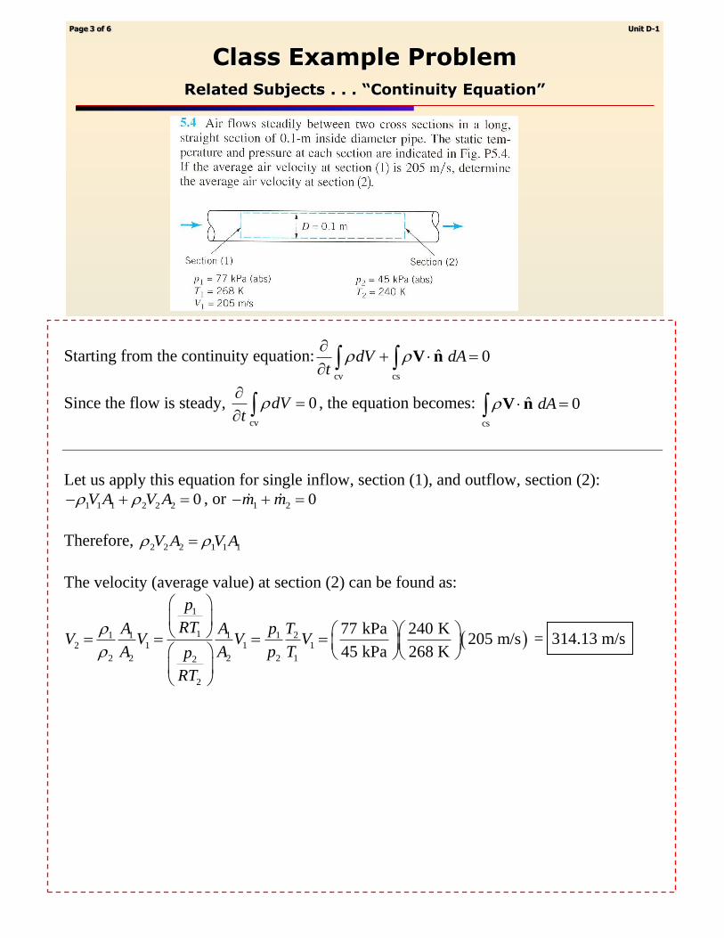
Starting from the continuity equation:cv cs
ˆ 0dV dAt
+ = V n
Since the flow is steady, cv
0dVt
=
, the equation becomes: cs
ˆ 0dA = V n
Let us apply this equation for single inflow, section (1), and outflow, section (2):
1 1 1 2 2 2 0V A V A − + = , or 1 2 0m m− + =
Therefore, 2 2 2 1 1 1V A V A =
The velocity (average value) at section (2) can be found as:
( )
1
11 1 1 1 22 1 1 1
2 2 2 2 12
2
77 kPa 240 K205 m/s
45 kPa 268 K
p
RTA A p TV V V V
A A p Tp
RT
= = = =
= 314.13 m/s
Unit D-1Page 3 of 6
Class Example Problem
Related Subjects . . . “Continuity Equation”

_________________________________________________________
_________________________________________________________
_________________________________________________________
_________________________________________________________
_________________________________________________________
_________________________________________________________
_________________________________________________________
_________________________________________________________
_________________________________________________________
_________________________________________________________
_________________________________________________________
_________________________________________________________
_________________________________________________________
_________________________________________________________
_________________________________________________________
_________________________________________________________
_________________________________________________________
_________________________________________________________
_________________________________________________________
_________________________________________________________
_________________________________________________________
_________________________________________________________
_________________________________________________________
_________________________________________________________
_________________________________________________________
_________________________________________________________
Starting from the continuity equation:cv cs
ˆ 0dV dAt
+ = V n
As a fixed control volume is defined (the bathtub), the flow within the control volume is
NOT steady (it will change the mass over time).
air air air water water water
air water volume volume
0dV m dV mt t
+ + − =
Let us consider only the flow of water (since we are interested in water depth):
water water water
water volume
0dV mt
− =
Note that: ( )( ) ( )water water water
water volume
2 ft 5 ft 1.5 ft jdV h h A = + −
Therefore, ( )( ) ( ) water water2 ft 5 ft 1.5 ft jh h A mt
+ − =
or, ( )2
water water water10 ft j
hA m Q
t
− = =
Hence, ( ) ( )
water water
2 210 ft 10 ftj
h Q Q
t A
=
− (since
210 ftjA )
The time rate of change of the water depth is:
( )
( )
( )
3
water
2 2
1 ft9 gal/min
7.48 gal 12 in
1 ft10 ft 10 ft
h Q
t
= =
= 1.44 in/min
Unit D-1Page 4 of 6
EXAMPLE 5.5Textbook (Munson, Young, and Okiishi), page 198
Conservation of Mass – Unsteady Flow
Unit D-1Page 5 of 6
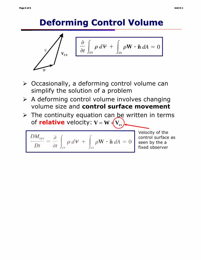
Deforming Control Volume
VCSUNIT EUNIT E--11SLIDE SLIDE 1515
Deforming Control VolumeDeforming Control Volume
➢ Occasionally, a deforming control volume can simplify the solution of a problem
➢ A deforming control volume involves changing volume size and control surface movement
➢ The continuity equation can be written in terms of relative velocity: scVWV +=
Velocity of the control surface as seen by the a fixed observer
_________________________________________________________
_________________________________________________________
_________________________________________________________
_________________________________________________________
_________________________________________________________
_________________________________________________________
_________________________________________________________
_________________________________________________________
_________________________________________________________
_________________________________________________________
_________________________________________________________
_________________________________________________________
_________________________________________________________
_________________________________________________________
_________________________________________________________
_________________________________________________________
_________________________________________________________
_________________________________________________________
_________________________________________________________
_________________________________________________________
_________________________________________________________
_________________________________________________________
_________________________________________________________
_________________________________________________________
_________________________________________________________
_________________________________________________________
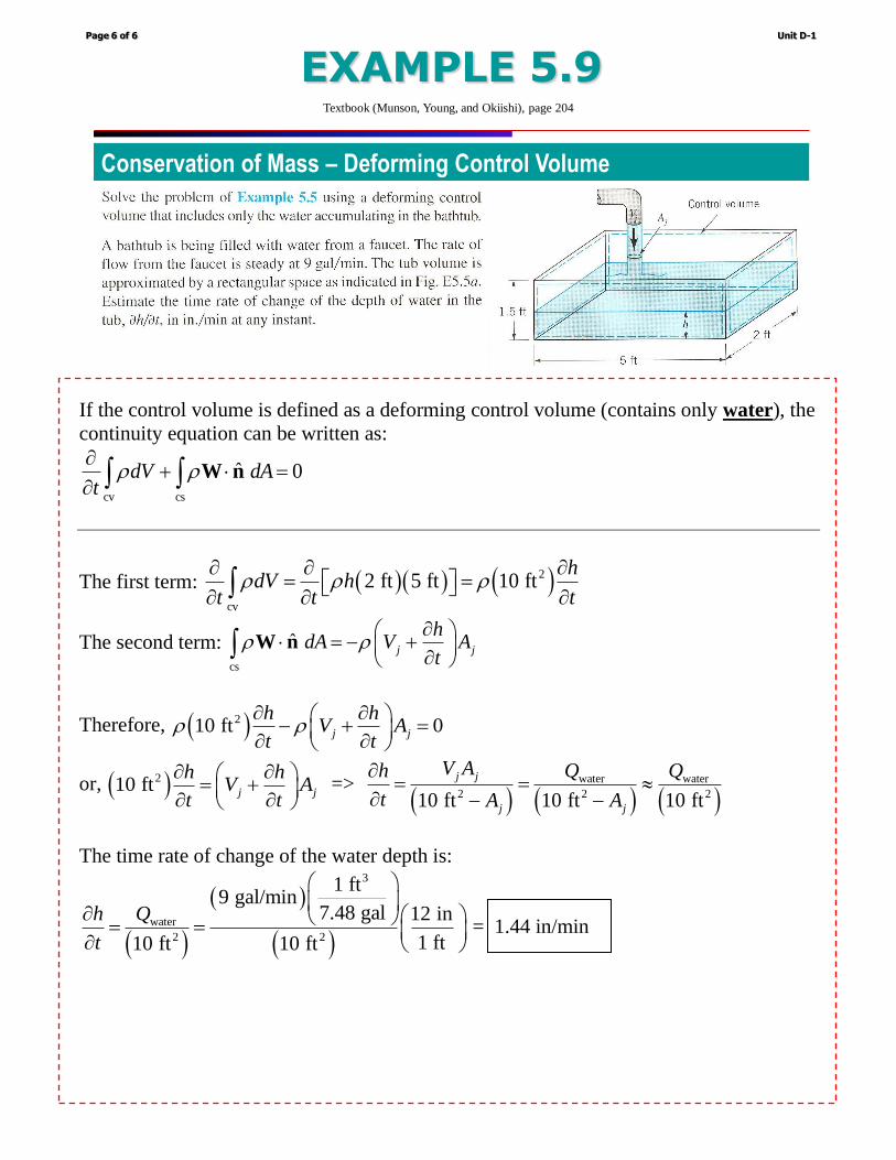
If the control volume is defined as a deforming control volume (contains only water), the
continuity equation can be written as:
cv cs
ˆ 0dV dAt
+ = W n
The first term: ( )( ) ( )2
cv
2 ft 5 ft 10 fth
dV ht t t
= =
The second term: cs
ˆ j j
hdA V A
t
= − +
W n
Therefore, ( )210 ft 0j j
h hV A
t t
− + =
or, ( )210 ft j j
h hV A
t t
= +
=>
( ) ( ) ( )water water
2 2 210 ft 10 ft 10 ft
j j
j j
V Ah Q Q
t A A
= =
− −
The time rate of change of the water depth is:
( )
( )
( )
3
water
2 2
1 ft9 gal/min
7.48 gal 12 in
1 ft10 ft 10 ft
h Q
t
= =
= 1.44 in/min
Unit D-1Page 6 of 6
EXAMPLE 5.9Textbook (Munson, Young, and Okiishi), page 204
Conservation of Mass – Deforming Control Volume
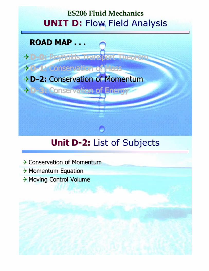
ES206 Fluid Mechanics
UNIT D: Flow Field Analysis
ROAD MAP . . .
D-0: Reynolds Transport Theorem
D-1: Conservation of Mass
D-2: Conservation of Momentum
D-3: Conservation of Energy
ES206 Fluid Mechanics
Unit D-2: List of Subjects
Conservation of Momentum
Momentum Equation
Moving Control Volume

_________________________________________________________
_________________________________________________________
_________________________________________________________
_________________________________________________________
_________________________________________________________
_________________________________________________________
_________________________________________________________
_________________________________________________________
_________________________________________________________
_________________________________________________________
_________________________________________________________
_________________________________________________________
_________________________________________________________
_________________________________________________________
_________________________________________________________
_________________________________________________________
_________________________________________________________
_________________________________________________________
_________________________________________________________
_________________________________________________________
_________________________________________________________
_________________________________________________________
_________________________________________________________
_________________________________________________________
Unit D-2Page 1 of 7
Conservation of Momentum
Time rate of change of the linear momentum of the System
Time rate of change of the linear momentum of the contents of the control volume
Net rate of flow of linear momentum through the control surface
= +
UNIT EUNIT E--22SLIDE SLIDE 22
Linear Momentum EquationLinear Momentum Equation (1)(1)
➢ For a system and a fixed, non-deforming cv that are coincident at an instant of time (t), the Reynolds transport theorem with B = momentum
(mass times velocity) and b = V provides:
Textbook (Munson, Young, and Okiishi), page 205
UNIT EUNIT E--22SLIDE SLIDE 11
NewtonNewton’’s Second Laws Second Law
➢ Newton’s second law of motion states:
➢ Since momentum is mass times velocity, the momentum of a small particle of mass is:
➢ Thus, the momentum of the entire system is:
➢ Newton’s second law is:
➢ Any reference or coordinate system for which this statement is true is called inertial
➢ A fixed coordinate system is inertial
➢ A coordinate system that moves in a straight line with
constant velocity is also inertial
Time rate of change of the linear momentum of the system
=Sum of external forces acting on the system
UNIT EUNIT E--22SLIDE SLIDE 33
➢ The conservation of momentum is simply, “time rate of change of the linear momentum of the system = sum of external forces acting on the system”
Linear Momentum EquationLinear Momentum Equation (2)(2)
Time rate of change of the linear momentum of the System
Time rate of change of the linear momentum of the contents of the control volume
Net rate of flow of linear momentum through the control surface
= +
where,
(Linear Momentum Equation)

Unit D-2Page 2 of 7
Momentum Equation
(2) External Forces (3) Sign Convention(1) Coordinate System
UNIT EUNIT E--22SLIDE SLIDE 88
Application of Momentum Application of Momentum
EquationEquation (1)(1)
➢ When the flow is uniformly distributed over a section of the control surface (1-D flow) where flow into or out of the control volume occurs, the integral operations are simplified
➢ Linear momentum is directional
➢ The flow of positive or negative linear momentum into a control volume can be determined by the dot product:
➢ Time rate of change of the linear momentum of the contents of a non-deforming control volume is zero for steady flow
➢ The forces due to atmospheric pressure acting on the control surface may need consideration
nV ˆ
UNIT EUNIT E--22SLIDE SLIDE 99
Application of Momentum Application of Momentum
EquationEquation (2)(2)
➢ If the control surface is selected so that it is perpendicular to the flow where fluid enters or exits the control volume, the surface force exerted at these locations by fluid outside the control volume on fluid inside will be due to pressure
➢ The external forces have an algebraic sign, positive if the force is in the assigned positive coordinate direction and negative otherwise
➢ Only external forces acting on the contents of the control volume are considered in the linear momentum equation
➢ The force required to anchor an object will generally exist in response to surface pressure and/or shear forces acting on the control surface
_________________________________________________________
_________________________________________________________
_________________________________________________________
_________________________________________________________
_________________________________________________________
_________________________________________________________
_________________________________________________________
_________________________________________________________
_________________________________________________________
_________________________________________________________
_________________________________________________________
_________________________________________________________
_________________________________________________________
_________________________________________________________
_________________________________________________________
_________________________________________________________
_________________________________________________________
_________________________________________________________
_________________________________________________________
_________________________________________________________
_________________________________________________________
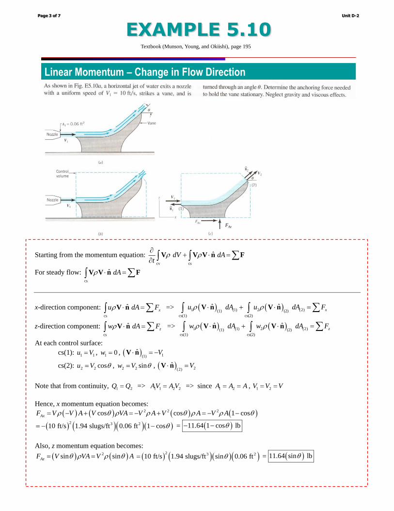
Starting from the momentum equation: cv cs
ˆ dV dAt
+ =
V V V n F
For steady flow: cs
ˆ dA =V V n F
x-direction component: cs
ˆ xu dA F = V n => ( ) ( )1 (1) 2 (2)(1) (2)
cs(1) cs(2)
ˆ ˆ xu dA u dA F + = V n V n
z-direction component: cs
ˆ zw dA F = V n => ( ) ( )1 (1) 2 (2)(1) (2)
cs(1) cs(2)
ˆ ˆ zw dA w dA F + = V n V n
At each control surface:
cs(1): 1 1u V= , 1 0w = , ( ) 1(1)ˆ V = −V n
cs(2): 2 2 cosu V = , 2 2 sinw V = , ( ) 2(2)ˆ V =V n
Note that from continuity, 1 2Q Q= => 1 1 2 2AV A V= => since 1 2A A A= = , 1 2V V V= =
Hence, x momentum equation becomes:
( ) ( ) ( ) ( )2 2 2cos cos 1 cosAxF V V A V VA V A V A V A = − + = − + = − −
( ) ( )( )( )2 3 210 ft/s 1.94 slugs/ft 0.06 ft 1 cos= − − = ( )11.64 1 cos lb− −
Also, z momentum equation becomes:
( ) ( )2sin sinAzF V VA V A = = ( ) ( )( )( )2 3 210 ft/s 1.94 slugs/ft sin 0.06 ft= = ( )11.64 sin lb
Unit D-2Page 3 of 7
EXAMPLE 5.10Textbook (Munson, Young, and Okiishi), page 195
Linear Momentum – Change in Flow Direction
FAz
_________________________________________________________
_________________________________________________________
_________________________________________________________
_________________________________________________________
_________________________________________________________
_________________________________________________________
_________________________________________________________
_________________________________________________________
_________________________________________________________
_________________________________________________________
_________________________________________________________
_________________________________________________________
_________________________________________________________
_________________________________________________________
_________________________________________________________
_________________________________________________________
_________________________________________________________
_________________________________________________________
_________________________________________________________
_________________________________________________________
_________________________________________________________
_________________________________________________________
_________________________________________________________
_________________________________________________________
_________________________________________________________
Starting from the momentum equation: cv cs
ˆ dV dAt
+ =
V V V n F
For steady flow: cs
ˆ dA =V V n F
x-direction component: cs
ˆ xu dA F = V n
=> ( ) ( ) ( )1 (1) 2 (2) 3 (3)(1) (2) (3)
cs(1) cs(2) cs(3)
ˆ ˆ ˆ xu dA u dA u dA F + + = V n V n V n
y-direction component: cs
ˆ yv dA F = V n
=> ( ) ( ) ( )1 (1) 2 (2) 3 (3)(1) (2) (3)
cs(1) cs(2) cs(3)
ˆ ˆ ˆ yv dA v dA v dA F + + = V n V n V n
At each control surface:
cs(1): 1u V= , 1 0v = , ( )(1)
ˆ V = −V n
cs(2): 2 cos30u V= , 2 sin 30v V= − , ( )(2)
ˆ V =V n
cs(3): 3u V= , 3 0v = , ( )(3)
ˆ V =V n
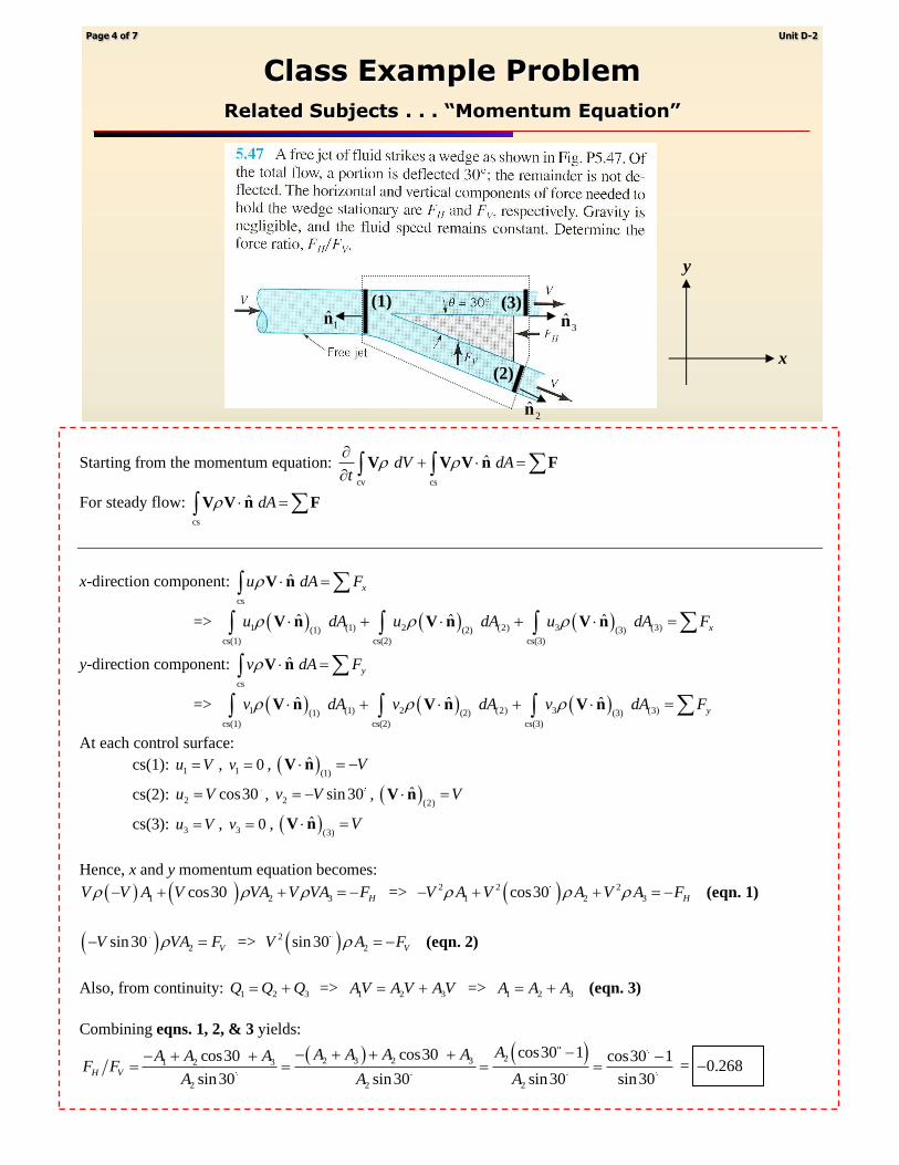
Hence, x and y momentum equation becomes:
( ) ( )1 2 3cos30 HV V A V VA V VA F − + + = − => ( )2 2 2
1 2 3cos30 HV A V A V A F − + + = − (eqn. 1)
( ) 2sin30 VV VA F− = => ( )2
2sin30 VV A F = − (eqn. 2)
Also, from continuity: 1 2 3Q Q Q= + => 1 2 3AV A V A V= + => 1 2 3A A A= + (eqn. 3)
Combining eqns. 1, 2, & 3 yields:
( ) ( )22 3 2 31 2 3
2 2 2
cos30 1cos30cos30 cos30 1
sin30 sin30 sin30 sin30H V
AA A A AA A AF F
A A A
−− + + +− + + −= = = = = −0.268
Unit D-2Page 4 of 7
Class Example Problem
Related Subjects . . . “Momentum Equation”
(1) (3)
(2)
1n̂
2n̂
3n̂
y
x

_________________________________________________________
_________________________________________________________
_________________________________________________________
_________________________________________________________
_________________________________________________________
_________________________________________________________
_________________________________________________________
_________________________________________________________
_________________________________________________________
_________________________________________________________
_________________________________________________________
_________________________________________________________
_________________________________________________________
_________________________________________________________
_________________________________________________________
_________________________________________________________
_________________________________________________________
_________________________________________________________
_________________________________________________________
_________________________________________________________
Starting from the momentum equation: cv cs
ˆ dV dAt
+ =
V V V n F
For steady flow: cs
ˆ dA =V V n F
x-direction component: cs
ˆ xu dA F = V n => ( ) ( )1 (1) 2 (2)(1) (2)
cs(1) cs(2)
ˆ ˆ xu dA u dA F + = V n V n
At each control surface:
cs(1): 1 1u V= , ( ) 1(1)ˆ V = −V n
cs(2): 2 2 sin 20u V= , ( ) 2(2)ˆ V =V n
Hence, x momentum equation becomes:
( ) ( )1 1 1 2 2 2 water 1 1
1sin 20 cos20
2Ax Rx AxV V A V V A F F F h A
− + = − + = − +
=> ( )2 2
1 1 2 2 water 1 1
1sin 20 cos20
2AxV A V A F h A − + = − + (eqn. 1)
Also, from continuity: 1 2Q Q= => 1 1 2 2AV A V= => 1 12 1 1
2 2
A hV V V
A h= = (eqn. 2)
Combining eqns. 1 & 2 yields (note that in terms of “per unit depth,” 1 1A h→ & 2 2A h→ ):
( ) ( )2
2 2 1water 1 1 1 1 2
2
1cos20 sin 20
2Ax
hF h V h V h
h
= + −
( )( ) ( ) ( ) ( )( ) ( ) ( )( )( )2
2 23 3 31 4 ft62.4 lb/ft 4 ft cos20 10 ft/s 1.94 slugs/ft 4 ft 10 ft/s sin 20 1.94 slugs/ft 1 ft
2 1 ft
= + −
= 183.46 lb
Unit D-2Page 5 of 7
Class Example Problem
Related Subjects . . . “Momentum Equation”
(1)
(2)
1n̂
2n̂
y
x FR
Unit D-2Page 6 of 7
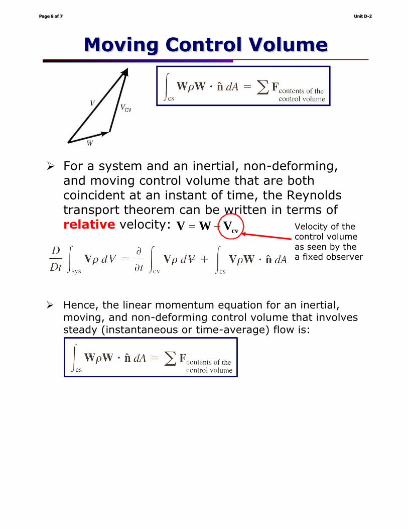
Moving Control VolumeUNIT EUNIT E--22SLIDE SLIDE 1414
Moving Control VolumeMoving Control Volume (1)(1)
➢ A stationary non-deforming control volume is inertial (no acceleration)
➢ A non-deforming control volume translating in a straight line at constant speed is also inertial
➢ For a system and an inertial, non-deforming, and moving control volume that are both coincident at an instant of time, the Reynolds transport theorem can be written in terms of relative velocity:
cvVWV += Velocity of the control volume as seen by the a fixed observer
UNIT EUNIT E--22SLIDE SLIDE 1717
➢ For inertial non-deforming control volume:
➢ For steady flow (on an instantaneous or time-average basis), it can be simplified as:
➢ Hence, the linear momentum equation for an inertial, moving, and non-deforming control volume that involves steady (instantaneous or time-average) flow is:
Moving Control VolumeMoving Control Volume (4)(4)

Unit EUnit E--22Page Page 88 of 8of 8
EXAMPLE 5.17EXAMPLE 5.17Textbook (Munson, Young, and Okiishi), page 219
Linear Momentum – Moving Control Volume
_________________________________________________________
_________________________________________________________
_________________________________________________________
_________________________________________________________
_________________________________________________________
_________________________________________________________
_________________________________________________________
_________________________________________________________
_________________________________________________________
_________________________________________________________
_________________________________________________________
_________________________________________________________
_________________________________________________________
_________________________________________________________
_________________________________________________________
_________________________________________________________
_________________________________________________________
_________________________________________________________
_________________________________________________________
_________________________________________________________
_________________________________________________________
_________________________________________________________
_________________________________________________________
For a moving control volume: cs
ˆ dA =W W n F
x-direction component: cs
ˆ x xW dA F = W n => ( ) ( )1 1 1 2 2 2cos45 xW W A W W A R − + = −
z-direction component: cs
ˆ z zW dA F = W n => ( )2 2 2sin 45 zW W A R = (ignoring the weight of water)
From continuity, 1 2Q Q= => 1 1 2 2AW A W= => since 1 2A A A= = , 1 2W W W= =
where, 1 2 1 0 100 ft/s 20 ft/s 80 ft/sW W W V V= = = − = − =
Hence, x momentum equation becomes:
( ) ( ) ( ) ( )( )( )22 2 2 3 2cos45 1 cos45 80 ft/s 1.94 slugs/ft 0.006 ft 1 cos45xR W A W A W A = − = − = − = 21.82 lb
Also, z momentum equation becomes:
( ) ( ) ( )( )( )22 3 2sin 45 80 ft/s sin 45 1.94 slugs/ft 0.006 ftzR W A= = = 52.68 lb
Magnitude of the force, exerted by the water is:
( ) ( )2 2
21.82 52.68F R= = + = 57.02 lb
Direction of the force is:
1 1 52.68tan tan
21.82
z
x
R
R − −
= =
= 67.5
Unit D-2Page 7 of 7
EXAMPLE 5.17Textbook (Munson, Young, and Okiishi), page 219
Linear Momentum – Moving Control Volume
z
x Rx
52.68 lb
21.82 lb
F
R
67.5
Rz

ES206 Fluid Mechanics
UNIT D: Flow Field Analysis
ROAD MAP . . .
D-0: Reynolds Transport Theorem
D-1: Conservation of Mass
D-2: Conservation of Momentum
D-3: Conservation of Energy
ES206 Fluid Mechanics
Unit D-3: List of Subjects
Conservation of Energy
Energy Equation
_________________________________________________________
_________________________________________________________
_________________________________________________________
_________________________________________________________
_________________________________________________________
_________________________________________________________
_________________________________________________________
_________________________________________________________
_________________________________________________________
_________________________________________________________
_________________________________________________________
_________________________________________________________
_________________________________________________________
_________________________________________________________
_________________________________________________________
_________________________________________________________
_________________________________________________________
_________________________________________________________
_________________________________________________________
_________________________________________________________
_________________________________________________________
_________________________________________________________
_________________________________________________________
_________________________________________________________
_________________________________________________________
_________________________________________________________
_________________________________________________________
_________________________________________________________
2 2
net netin insys cv cs
ˆ 2 2
D V Ve dV u gz dV u gz dA Q W
Dt t
= + + + + + = +
V n
Unit D-3Page 1 of 5
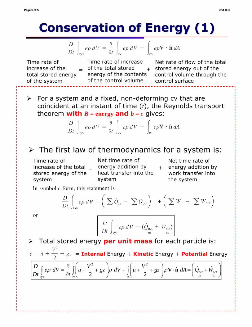
Conservation of Energy (1)
Time rate of increase of the total stored energy of the system
Time rate of increase of the total stored energy of the contents of the control volume
Net rate of flow of the total stored energy out of the control volume through the control surface
= +
UNIT EUNIT E--33SLIDE SLIDE 33
First Law of ThermodynamicsFirst Law of Thermodynamics (3)(3)
➢ For a system and a fixed, non-deforming cv that are coincident at an instant of time (t), the Reynolds transport theorem with B = energy and b = e gives:
➢ For a control volume that is fixed and non-deforming, the energy equation becomes:
Time rate of increase of the total stored energy of the system
Time rate of increase of the total stored energy of the contents of the control volume
Net rate of flow of the total stored energy out of the control volume through the control surface
= +
UNIT EUNIT E--33SLIDE SLIDE 11
➢ The first law of thermodynamics for a system is:
➢ Total stored energy per unit mass for each particle is:
First Law of ThermodynamicsFirst Law of Thermodynamics (1)(1)
Time rate of increase of the total stored energy of the system
Net time rate of energy addition by heat transfer into the system
Net time rate of energy addition by work transfer into the system
= +
= Internal Energy + Kinetic Energy + Potential Energy

_________________________________________________________
_________________________________________________________
_________________________________________________________
_________________________________________________________
_________________________________________________________
_________________________________________________________
_________________________________________________________
_________________________________________________________
_________________________________________________________
_________________________________________________________
_________________________________________________________
_________________________________________________________
_________________________________________________________
_________________________________________________________
_________________________________________________________
_________________________________________________________
_________________________________________________________
_________________________________________________________
_________________________________________________________
_________________________________________________________
_________________________________________________________
_________________________________________________________
_________________________________________________________
_________________________________________________________
Unit D-3Page 2 of 5
Conservation of Energy (2)
UNIT EUNIT E--33SLIDE SLIDE 33
First Law of ThermodynamicsFirst Law of Thermodynamics (3)(3)
➢ For a system and a fixed, non-deforming cv that are coincident at an instant of time (t), the Reynolds transport theorem with B = energy and b = e gives:
➢ For a control volume that is fixed and non-deforming, the energy equation becomes:
Time rate of increase of the total stored energy of the system
Time rate of increase of the total stored energy of the contents of the control volume
Net rate of flow of the total stored energy out of the control volume through the control surface
= +UNIT EUNIT E--33SLIDE SLIDE 44
➢ For a rotating shaft, the power transfer is related to the shaft torque and angular velocity:
➢ When the control surface cuts through the shaft material, the shaft torque is exerted by shaft material at the control surface:
➢ Work transfer can also occur at the control surface when a force associated with fluid normal stress acts over a distance – in case of the simple pipe flow:
First Law of ThermodynamicsFirst Law of Thermodynamics (4)(4)
Textbook (Munson, Young, and Okiishi), page 231
(Flow Work)
UNIT EUNIT E--33SLIDE SLIDE 55
First Law of ThermodynamicsFirst Law of Thermodynamics (5)(5)
➢ Including the flow work, the energy equation can be written as:
➢ Combining the flow work into the total energy:
(“Modified” Energy Equation)
innet W
Flow Work
net shaft normalin net in stress
W W W= +
_________________________________________________________
_________________________________________________________
_________________________________________________________
_________________________________________________________
_________________________________________________________
_________________________________________________________
_________________________________________________________
_________________________________________________________
_________________________________________________________
_________________________________________________________
_________________________________________________________
_________________________________________________________
_________________________________________________________
_________________________________________________________
_________________________________________________________
_________________________________________________________
_________________________________________________________
_________________________________________________________
_________________________________________________________
_________________________________________________________
_________________________________________________________
_________________________________________________________
_________________________________________________________
_________________________________________________________
_________________________________________________________
_________________________________________________________
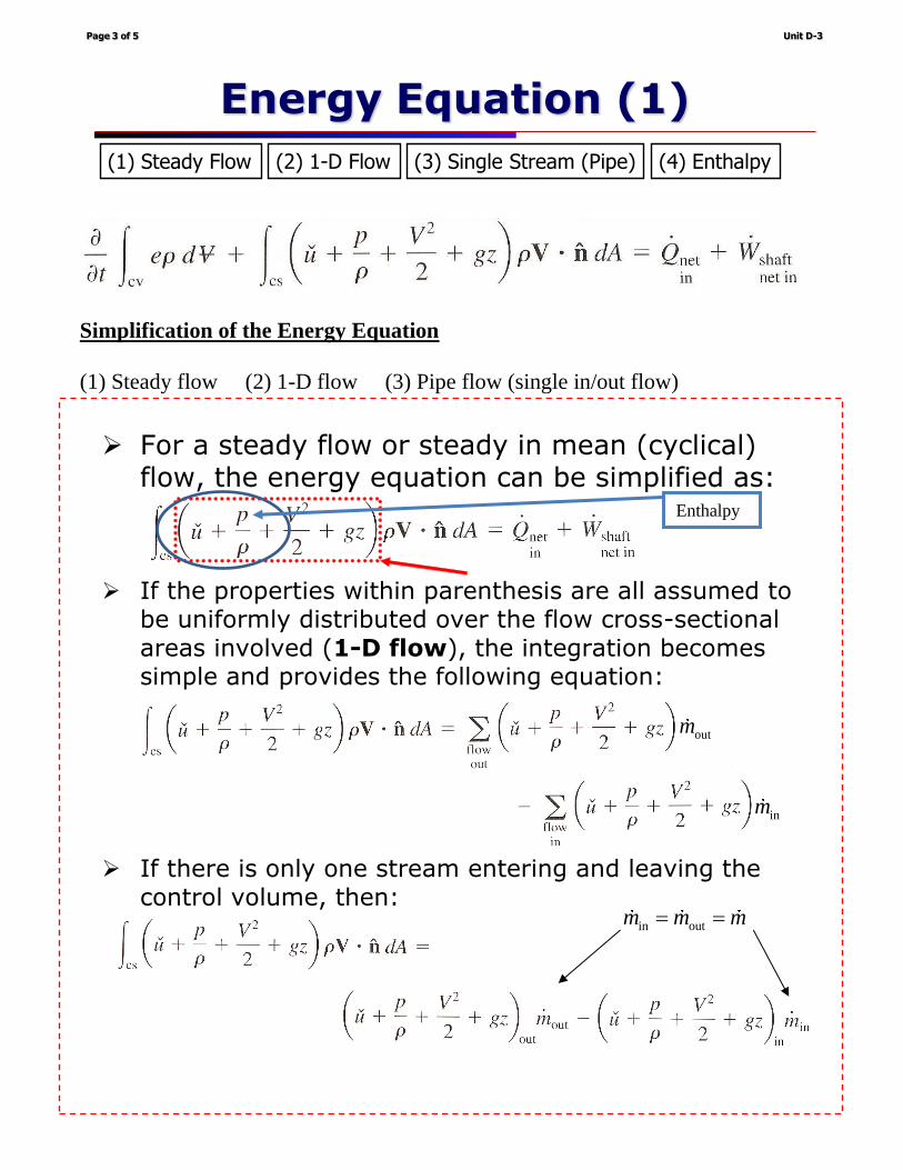
Simplification of the Energy Equation
(1) Steady flow (2) 1-D flow (3) Pipe flow (single in/out flow)
Unit D-3Page 3 of 5
Energy Equation (1)
(2) 1-D Flow (3) Single Stream (Pipe)(1) Steady Flow (4) Enthalpy
Unit D-3Page 2 of 5
Conservation of Energy (2)
UNIT EUNIT E--33SLIDE SLIDE 66
Energy EquationEnergy Equation (1)(1)
➢ For a steady flow or steady in mean (cyclical) flow, the energy equation can be simplified as:
➢ If the properties within parenthesis are all assumed to be uniformly distributed over the flow cross-sectional areas involved (1-D flow), the integration becomes simple and provides the following equation:
UNIT EUNIT E--33SLIDE SLIDE 77
Energy EquationEnergy Equation (2)(2)
➢ If there is only one stream entering and leaving the control volume, then:
Textbook (Munson, Young, and Okiishi), page 233
Uniform flow (1-D) will occur in an infinitesimally small diameter streamtube – the streamtubeflow is representative of the steady flow of a particle of fluid along a pathline
in outm m m= =
outm
inm
Enthalpy
_________________________________________________________
_________________________________________________________
_________________________________________________________
_________________________________________________________
_________________________________________________________
_________________________________________________________
_________________________________________________________
_________________________________________________________
_________________________________________________________
_________________________________________________________
_________________________________________________________
_________________________________________________________
_________________________________________________________
_________________________________________________________
_________________________________________________________
_________________________________________________________
_________________________________________________________
_________________________________________________________
_________________________________________________________
_________________________________________________________
_________________________________________________________
_________________________________________________________
_________________________________________________________
_________________________________________________________
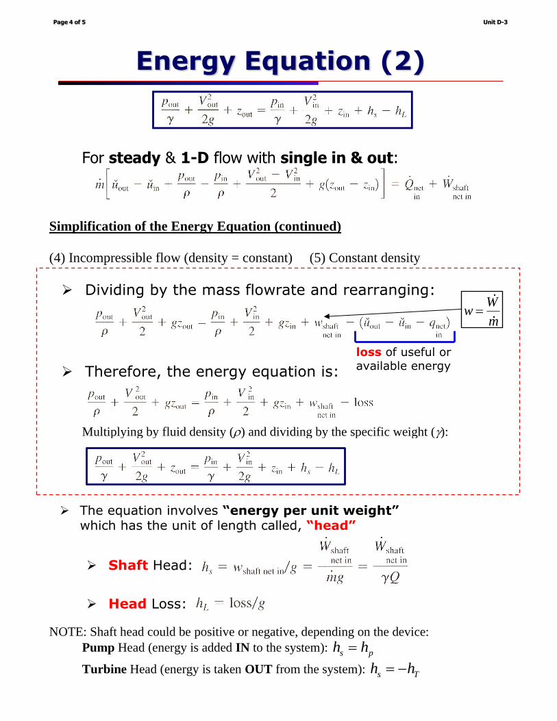
For steady & 1-D flow with single in & out:
Simplification of the Energy Equation (continued)
(4) Incompressible flow (density = constant) (5) Constant density
Multiplying by fluid density () and dividing by the specific weight ():
NOTE: Shaft head could be positive or negative, depending on the device:
Pump Head (energy is added IN to the system): s ph h=
Turbine Head (energy is taken OUT from the system): s Th h= −
Unit D-3Page 4 of 5
Energy Equation (2)UNIT EUNIT E--33SLIDE SLIDE 1616
➢ For 1-D steady flow energy equation, if the shaft power input is included:
➢ Dividing by the mass flowrate and rearranging:
➢ Therefore, the energy equation is:
Energy LossEnergy Loss (2)(2)
loss of useful or available energy
(Mechanical Energy Equation)
UNIT EUNIT E--33SLIDE SLIDE 1616
➢ For 1-D steady flow energy equation, if the shaft power input is included:
➢ Dividing by the mass flowrate and rearranging:
➢ Therefore, the energy equation is:
Energy LossEnergy Loss (2)(2)
loss of useful or available energy
(Mechanical Energy Equation)
UNIT EUNIT E--33SLIDE SLIDE 1616
➢ For 1-D steady flow energy equation, if the shaft power input is included:
➢ Dividing by the mass flowrate and rearranging:
➢ Therefore, the energy equation is:
Energy LossEnergy Loss (2)(2)
loss of useful or available energy
(Mechanical Energy Equation)
UNIT EUNIT E--33SLIDE SLIDE 1717
➢ Recall, the mechanical energy equation:
➢ Multiplying by fluid density:
➢ Dividing by the specific weight:
➢ The equation involves “energy per unit weight”which has the unit of length called, “head”
Energy LossEnergy Loss (3)(3)
g =
(Energy Equation in Terms of Head)
UNIT EUNIT E--33SLIDE SLIDE 1818
➢ The energy equation:
➢ Shaft Head:
➢ Head Loss:
➢ Turbine Head:
➢ Pump Head:
Energy LossEnergy Loss (4)(4)
Ww
m=

_________________________________________________________
_________________________________________________________
_________________________________________________________
_________________________________________________________
_________________________________________________________
_________________________________________________________
_________________________________________________________
_________________________________________________________
_________________________________________________________
_________________________________________________________
_________________________________________________________
_________________________________________________________
_________________________________________________________
_________________________________________________________
_________________________________________________________
_________________________________________________________
_________________________________________________________
_________________________________________________________
_________________________________________________________
_________________________________________________________
_________________________________________________________
Starting from the energy equation:
2 2
out out in inout in
2g 2gs L
p V p Vz z h h
+ + = + + + −
Note that:
out 0p = (gage pressure)
out 0V = (velocity becomes zero, by reaching 60 ft elevation)
out 60 ftz = 2
2
in
12 in10 psi 10 1,440 lb/ft
1 ftp
= = =
(gage pressure)
( )
3
in 2
in
1.5 ft /s17.19 ft/s
1 ft4 in
4 12 in
QV
A = = =
in 0z =
0Lh = (head loss is ignored)
Therefore,
( )
( )
22 2
in inout 3 2
17.19 ft/s1,440 lb/ft60 ft 32.33 ft
2g 62.4 lb/ft 2 32.2 ft/ss p
p Vh h z
= = − − = − − =
( )( )( )3 3
shaftnet in
1 hp62.4 lb/ft 1.5 ft /s 32.33 ft
550 ft lb/ssW Qh
= =
= 5.5 hp
Unit D-3Page 5 of 5
Class Example Problem
Related Subjects . . . “Energy Equation”
z