Estimating Shelf Seawater Composition by Inversion of AC9 Inherent Optical Property Measurements

Ian C. Brown, Alex Cunningham, David McKeePhysics Department, University of Strathclyde, 107 Rottenrow, Glasgow, G4 0NG Scotland

ABSTRACT

Shelf seas are complex, dynamic systems, within which important physical and biological processes occur. Water composition information may be used to quantify and map these processes both spatially and temporally. This information is routinely obtained through laboratory sample analyses which have poor spatial and temporal resolution compared with those of other physical variables such as temperature and salinity. Proposed strategies for partitioning in situ absorption coefficient measurements between optically significant constituents include matrix inversion (Gallegos & Neale, 2002) and constrained, non-linear regression methods (Schofield et al, 2004). As an extension of these ideas, we have developed a sequential, mechanistic, specific IOP based approach to partition both in situ absorption and scattering coefficient measurements between constituents and subsequently retrieve constituent concentrations. A comparison of these inversion procedures is presented, demonstrating that our specific IOP based procedure performs comparably with the previously published matrix inversion algorithm, appropriately constrained. Both procedures were validated using synthetic IOPs prior to being applied to a diverse field data set. Our procedure was used to interpret vertical water column structure and identify complex patterns of phytoplankton and suspended sediment distribution in Scottish sea lochs. Degradation in constituent concentration retrieval was observed when these procedures were applied to field data. This is partly attributed to the use of a single set of specific IOPs and normalised absorption spectra in the inversion of field data from a wide range of coastal waters. Accounting for variability in specific absorption and scattering properties of optically significant constituents may improve constituent retrievals regardless of the inversion method employed.

INTRODUCTION

Absorption, scattering and beam attenuation coefficients (a(λ), b(λ) and c(λ), respectively), together with the scattering phase function, , are collectively known as the inherent optical properties (IOPs) of seawater. The magnitude and spectral variation of in situ IOPs are determined by the concentration and chemical composition of dissolved and suspended materials present in seawater (Kirk, 1994). In addition to water itself, shelf seas are generally considered to contain three classes of optically significant constituents: phytoplankton (measured as chlorophyll a, CHL), mineral suspended solids (MSS) and coloured dissolved organic matter (CDOM). Information on water composition should allow the identification, quantification and mapping of various physical and biological processes both spatially and temporally. For example, CHL concentration is often used as a proxy for phytoplankton abundance and MSS concentration may be used to indicate sediment re-suspension and transport. Optically significant constituent concentrations are currently obtained through sample collection and laboratory analyses which are labour intensive and provide poor spatial and temporal coverage compared to that of other physical variables such as salinity and temperature. There is a need for development of supplementary methods of determining water composition to provide comparable coverage to that of other physical variables. The high sampling rate and relative ease of deployment suggest that in situ optics would provide a suitable basis for such procedures. As in situ absorption and attenuation coefficient measurements (from which scattering is derived) are routinely made using

WETLabs AC-9 (and increasingly, AC-S) dual-beam spectrophotometers, and the magnitude and spectral variation of these inherent optical properties (IOPs) are determined by the concentration and composition of seawater constituents, IOP inversion is a prime candidate. Such inversion techniques, applied to in situ optical data obtained from moorings or towed-bodies, may provide useful insights into variability in water composition and shelf sea processes.

AC-9 data (aAC9(λ), bAC9(λ) and cAC9(λ)), are used in a wide range of applications including the quantification of variability in inherent and apparent optical properties of seawater (Astoreca et al, 2006; Whitmire et al, 2007), optical water type classification (McKee & Cunningham, 2006) and numerical modelling of the physical properties of natural particle assemblages (Boss et al, 2001; Twardowski et al, 2001). In addition, AC-9 data are frequently incorporated into radiance transfer calculations of water leaving radiances for use in remote sensing applications (Bulgarelli et al, 2003), (Chang et al, 2003) and optical closure studies (Barnard et al, 1999; McKee et al 2003, McKee and Cunningham 2005; Tzortziou et al, 2006). Despite extensive measurements, there are at present no generally accepted protocols to invert in situ IOP measurements to obtain water composition information. Models for the partitioning of particulate absorption coefficients between constituents, using the quantitative filter pad method have been proposed (Morrow et al, 1989; Bricaud and Stramski, 1990). Various methods have been proposed for the inversion of in situ non-water absorption coefficients to obtain constituent partitioned absorption coefficients and/or constituent concentrations. These include numerical decomposition (Roesler et al, 1989), non-linear constrained least squares regression (Schofield et al, 2004) and matrix inversion in conjunction with normalized constituent specific absorption spectra (Gallegos and Neale, 2002). The Roesler model (Roesler et al, 1989) makes the approximation that in situ absorption at 676 nm is entirely attributable to phytoplankton. Using the species dependent blue to red absorption ratio of phytoplankton, the summed absorption of MSS and CDOM was approximated algebraically. The combined spectral absorption of CDOM and non-algal particulates was then modelled using a single exponential. The contribution to absorption by phytoplankton was subsequently modelled by subtracting the modelled non-phytoplankton absorption from in situ absorption. The method proposed by Gallegos and Neale (2002) used matrix inversion and normalised mean absorption spectra to partition in situ absorption coefficients between phytoplankton, MSS and CDOM. The optical signal inversion method of Schofield et al (Schofield et al, 2004) used nonlinear, constrained least-squares regression to determine the optical weights of three classes of phytoplankton, together with the optical weights and spectral slopes of absorption by CDOM and detritus. With the exception of the Gallegos and Neale models, both in situ absorption partitioning models discussed above assume that phytoplankton is the dominant, or indeed sole, absorbing constituent at red wavelengths. While often true, this is not an invariably justifiable assumption, for instance, in turbid estuaries such as the Bristol Channel where the in situ absorption coefficient signal is driven by suspended mineral particles. Certain absorption partitioning models require a more detailed knowledge of the phytoplankton community structure than is often available. The model of Roesler et al, requires the specification of a single spectral slope to describe the cumulative absorption by CDOM and non-algal particulates. This is undesirable as this makes a priori assumptions regarding the composition of these materials and their relative concentration. Ancillary CDOM absorption measurements may be used to aid the discrimination of absorption by CDOM and MSS, however filtered AC-9 deployment or laboratory measurement of CDOM absorption coincident with in situ IOP measurements is not necessarily feasible, particularly for long-term time series applications.

This paper aims to investigate the extent to which shelf seawater constituent concentrations may be retrieved from in situ IOP measurements, by utilising prior knowledge of the specific absorption and scattering properties of discrete optically significant constituents. An IOP inversion procedure was

developed using constituent specific IOPs obtained from regression analyses to partition in situ absorption and scattering coefficients between phytoplankton, MSS and CDOM. The performance of this procedure was compared to that of the unconstrained matrix inversion method of Gallegos and Neale (2002). The performance degradation of each procedure in the presence of random noise was investigated using synthetic IOP data sets. A key objective was to test to what extent in situ IOPs could be successfully partitioned for a wide range of coastal waters using a single set of specific IOPs.

MEASUREMENTS

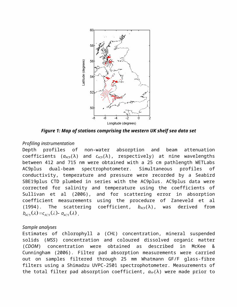
Between March 2000 and August 2006, 262 stations were occupied in the western UK shelf sea including Scottish Sea Lochs, the Irish and Celtic Seas and the Bristol Channel. Figure 1 shows a map of the locations of these stations.

Figure 1: Map of stations comprising the western UK shelf sea data set

Profiling instrumentationDepth profiles of non-water absorption and beam attenuation coefficients (aAC9(λ) and cAC9(λ), respectively) at nine wavelengths between 412 and 715 nm were obtained with a 25 cm pathlength WETLabs AC9plus dual-beam spectrophotometer. Simultaneous profiles of conductivity, temperature and pressure were recorded by a Seabird SBE19plus CTD plumbed in series with the AC9plus. AC9plus data were corrected for salinity and temperature using the coefficients of Sullivan et al (2006), and for scattering error in absorption coefficient measurements using the procedure of Zaneveld et al (1994). The scattering coefficient, bAC9(λ), was derived from

.

Sample analysesEstimates of chlorophyll a (CHL) concentration, mineral suspended solids (MSS) concentration and coloured dissolved organic matter (CDOM) concentration were obtained as described in McKee &

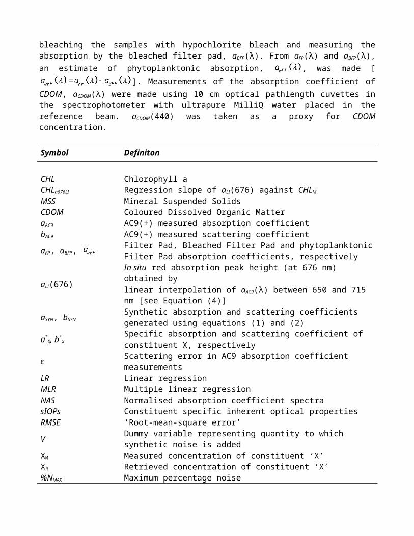
Cunningham (2006). Filter pad absorption measurements were carried out on samples filtered through 25 mm Whatmann GF/F glass-fibre filters using a Shimadzu UVPC-2501 spectrophotometer. Measurements of the total filter pad absorption coefficient, aFP(λ) were made prior to bleaching the samples with hypochlorite bleach and measuring the absorption by the bleached filter pad, aBFP(λ). From aFP(λ) and aBFP(λ), an estimate of phytoplanktonic absorption, , was made [

]. Measurements of the absorption coefficient of CDOM, aCDOM(λ) were made using 10 cm optical pathlength cuvettes in the spectrophotometer with ultrapure MilliQ water placed in the reference beam. aCDOM(440) was taken as a proxy for CDOM concentration.

Symbol Definiton

CHL Chlorophyll aCHLa676LI Regression slope of aLI(676) against CHLM MSS Mineral Suspended SolidsCDOM Coloured Dissolved Organic MatteraAC9 AC9(+) measured absorption coefficientbAC9 AC9(+) measured scattering coefficient

aFP, aBFP, Filter Pad, Bleached Filter Pad and phytoplanktonic Filter Pad absorption coefficients, respectively

aLI(676) In situ red absorption peak height (at 676 nm) obtained bylinear interpolation of aAC9(λ) between 650 and 715 nm [see Equation (4)]

aSYN, bSYNSynthetic absorption and scattering coefficients generated using equations (1) and (2)

a*X, b*

X Specific absorption and scattering coefficient of constituent X, respectivelyε Scattering error in AC9 absorption coefficient measurementsLR Linear regressionMLR Multiple linear regressionNAS Normalised absorption coefficient spectrasIOPs Constituent specific inherent optical propertiesRMSE ‘Root-mean-square error’V Dummy variable representing quantity to which synthetic noise is addedXM Measured concentration of constituent ‘X’XR Retrieved concentration of constituent ‘X’%NMAX Maximum percentage noise

Table 1: List of symbols used and definitions

METHODOLOGY

Pathlength amplification correctionAbsorption coefficients from filter pad optical density measurements were corrected for pathlength amplification by matching aFP(λ) to CDOM corrected AC9 absorption [aAC9(λ) - aCDOM(λ)] at each AC9 wavelength. This provided consistency between filter pad and AC9 absorption coefficient measurements.

Constituent specific IOPs (sIOPs)Constituent specific absorption coefficient spectra were obtained by linear (‘y-on-x’ ordinary least squares) regression of constituent absorption coefficients (from spectrophotometry) against measured constituent concentrations. Constituent specific scattering coefficient spectra were obtained through multiple linear regression of in situ scattering coefficients against measured CHL and MSS concentrations. These constituent specific IOPs are shown in Figure 2, with the data and regression techniques used in their derivation shown in Table 2.

Figure 2: Constituent specific IOPs: (a) specific absorption spectra obtained by linear regression of spectrophotometric absorption coefficient spectra, (b) specific scattering spectra from multiple linear regression of in situ scattering coefficients. Error bars represent the 95% confidence intervals in the regression slopes.

sIOP Method Dependent variable Independent variable(s)

a*CHL LR CHL

a*MSS LR aBFP(λ) MSS

a*CDOM LR aCDOM(λ) aCDOM(440)

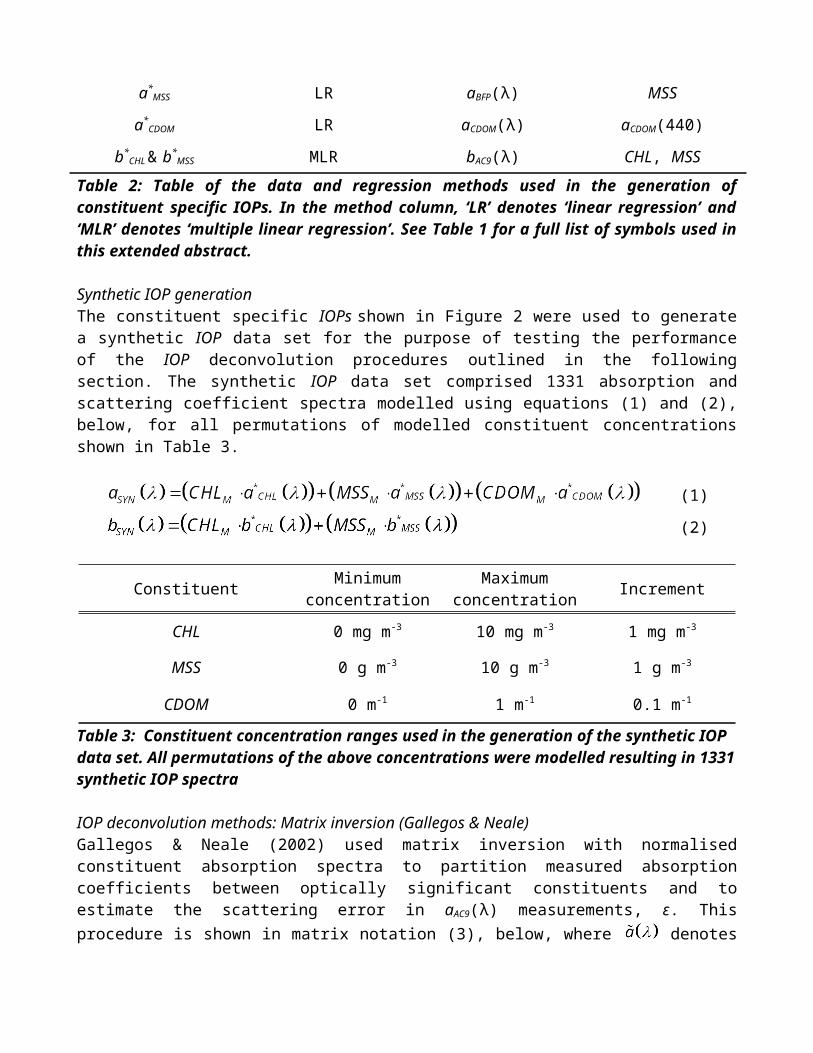
b*CHL & b*

MSS MLR bAC9(λ) CHL, MSS

Table 2: Table of the data and regression methods used in the generation of constituent specific IOPs. In the method column, ‘LR’ denotes ‘linear regression’ and ‘MLR’ denotes ‘multiple linear regression’. See Table 1 for a full list of symbols used in this extended abstract.

Synthetic IOP generationThe constituent specific IOPs shown in Figure 2 were used to generate a synthetic IOP data set for the purpose of testing the performance of the IOP deconvolution procedures outlined in the following section. The synthetic IOP data set comprised 1331 absorption and scattering coefficient spectra modelled using equations (1) and (2), below, for all permutations of modelled constituent concentrations shown in Table 3.

(1)

(2)

Constituent Minimum concentration

Maximum concentration Increment

CHL 0 mg m-3 10 mg m-3 1 mg m-3

MSS 0 g m-3 10 g m-3 1 g m-3

CDOM 0 m-1 1 m-1 0.1 m-1

Table 3: Constituent concentration ranges used in the generation of the synthetic IOP data set. All permutations of the above concentrations were modelled resulting in 1331 synthetic IOP spectra

IOP deconvolution methods: Matrix inversion (Gallegos & Neale)Gallegos & Neale (2002) used matrix inversion with normalised constituent absorption spectra to partition measured absorption coefficients between optically significant constituents and to estimate the scattering error in aAC9(λ) measurements, ε. This procedure is shown in matrix notation (3), below, where denotes normalised absorption spectra, and as a block diagram in Figure 3a. For consistency with the rest of this abstract, the notation has been changed from the original publication.

(3)

For this work, the matrix inversion procedure was modified to yield estimates of constituent concentrations from the partitioned absorption coefficient outputs using the constituent specific IOPs shown in Figure 2. Hereafter, the phrase ‘matrix inversion method’ is used to describe this modified matrix inversion method. It should be noted that only the unconstrained matrix inversion procedure has been implemented in the course of this work. A statistically augmented procedure was presented in which the contribution to in situ absorption by mineral particles was estimated from a relationship between pigment extracted filter pad absorption and in situ scattering coefficient measurements. Matrix inversion was subsequently employed to estimate aCHL(676) and aCDOM(440).

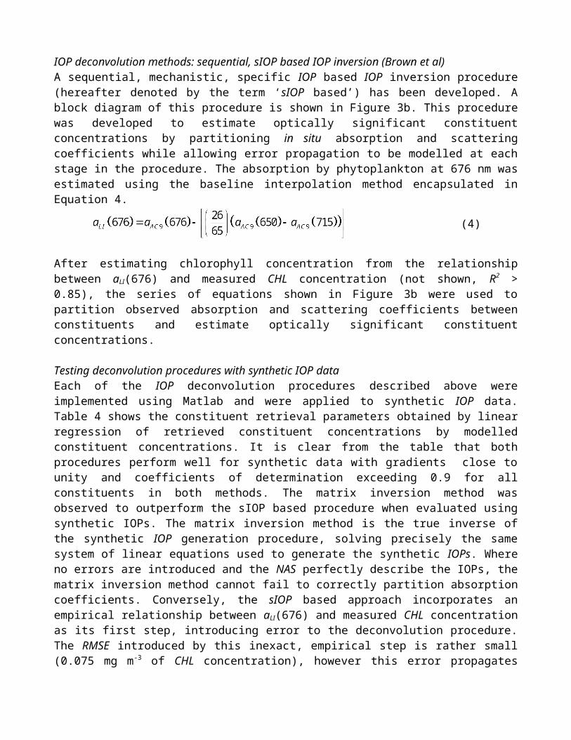
IOP deconvolution methods: sequential, sIOP based IOP inversion (Brown et al)A sequential, mechanistic, specific IOP based IOP inversion procedure (hereafter denoted by the term ‘sIOP based’) has been developed. A block diagram of this procedure is shown in Figure 3b. This procedure was developed to estimate optically significant constituent concentrations by partitioning in situ absorption and scattering coefficients while allowing error propagation to be modelled at each stage in the procedure. The absorption by phytoplankton at 676 nm was estimated using the baseline interpolation method encapsulated in Equation 4.

(4)

After estimating chlorophyll concentration from the relationship between aLI(676) and measured CHL concentration (not shown, R2 > 0.85), the series of equations shown in Figure 3b were used to partition observed absorption and scattering coefficients between constituents and estimate optically significant constituent concentrations.

Testing deconvolution procedures with synthetic IOP dataEach of the IOP deconvolution procedures described above were implemented using Matlab and were applied to synthetic IOP data. Table 4 shows the constituent retrieval parameters obtained by linear regression of retrieved constituent concentrations by modelled constituent concentrations. It is clear from the table that both procedures perform well for synthetic data with gradients close to unity and coefficients of determination exceeding 0.9 for all constituents in both methods. The matrix inversion method was observed to outperform the sIOP based procedure when evaluated using synthetic IOPs. The matrix inversion method is the true inverse of the synthetic IOP generation procedure, solving precisely the same system of linear equations used to generate the synthetic IOPs. Where no errors are introduced and the NAS perfectly describe the IOPs, the matrix inversion method cannot fail to correctly partition absorption coefficients. Conversely, the sIOP based approach incorporates an empirical relationship between aLI(676) and measured CHL concentration as its first step, introducing error to the deconvolution procedure. The RMSE introduced by this inexact, empirical step is rather small (0.075 mg m-3 of CHL concentration), however this error propagates through the procedure resulting in a more significant RMSE in CDOM absorption, hence CDOM concentration. The sequential nature of the sIOP based procedure allows errors to be tracked through each step of the procedure to observe the accumulation of error and potentially the sensitivity of the procedure to each sIOP and its associated variability. The matrix inversion procedure is less mathematically transparent making it more challenging to model the effects of error propagation on absorption partitioning.

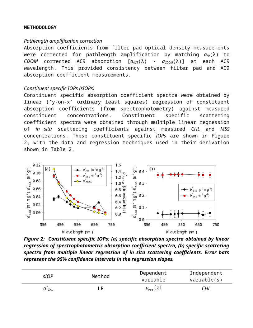
Figure 3: Block diagrams of IOP deconvolution procedures. (a) Gallegos & Neale ‘matrix inversion method’, (b) Brown et al, ‘sIOP based sequential method’. In panel (a) those operations enclosed in red borders are the necessary modifications to yield estimates of constituent concentrations from the standard matrix inversion outputs (partitioned absorption coefficients).

Method Constituent Retrieval Gradient Offset R2 RMSE

sIOP basedsIOP basedsIOP based

Matrix inversionMatrix inversionMatrix inversion

CHLMSS

CDOMCHLMSS

CDOM

0.9870.9991.0021.0000.9991.000

0.094-0.0030.1600.0010.0000.000

0.9990.9990.9070.9990.9990.999

0.075 mg m-3

0.190 g m-3

0.010 m-1

0.007 mg m-3

0.009 g m-3

0.000 m-1

Table 4: Constituent retrieval parameters obtained by regressing retrieved constituent concentration by modelled constituent concentration. RMSE is used to denote ‘root-mean-square error’.

IOP deconvolution procedures: noise sensitivityThe synthetic IOP data set discussed above was used to determine the sensitivity of each procedure to random noise in synthetic IOPs and random noise in sIOPs (or NAS). Uniformly distributed random noise was generated using Matlab and applied to synthetic IOPs, sIOPs and NAS as shown in Equation (5), wherein V is a dummy variable representing the variable to which noise is to be added. Subscript ‘NA’ denotes ‘noise added’ and %NMAX, is the maximum percentage noise in V.

(5)

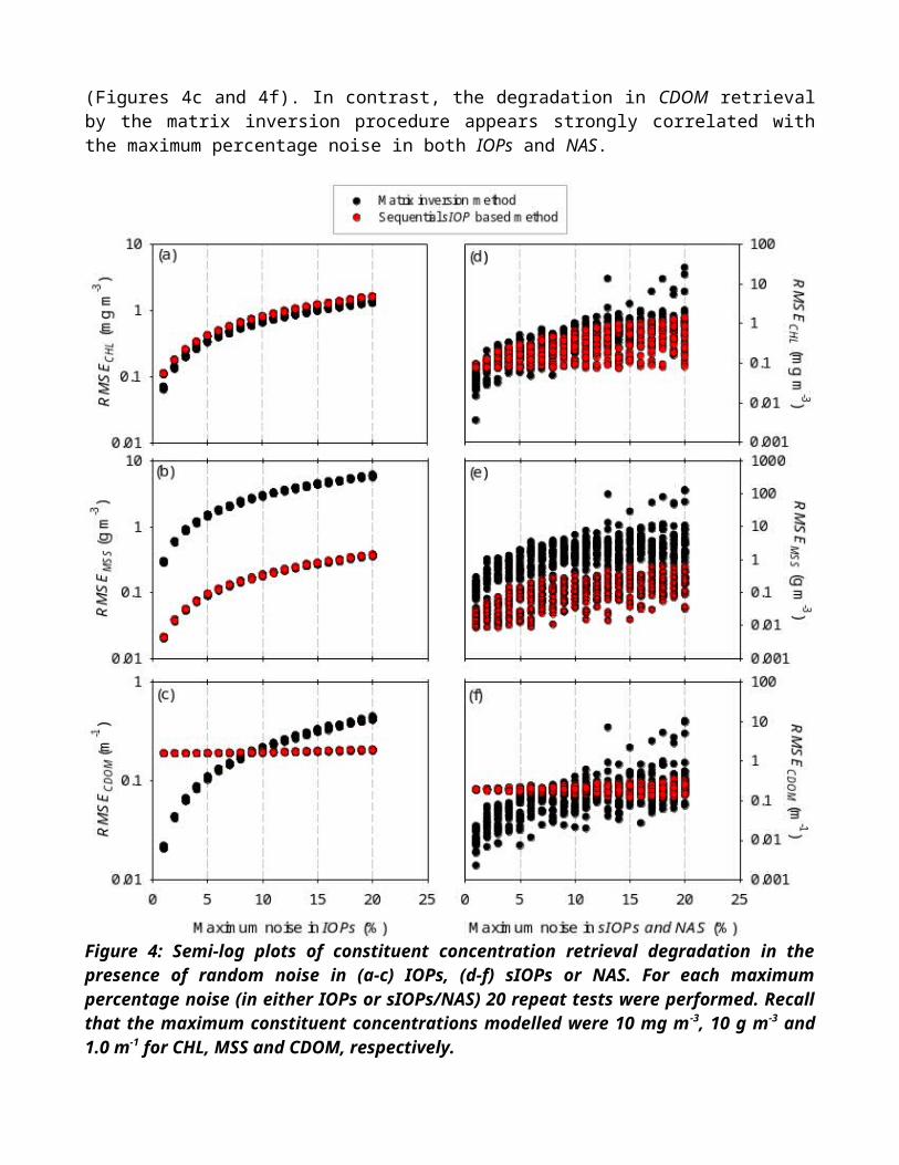
Each procedure was tested by sweeping %NMAX in synthetic IOPs and sIOPs and NAS from 1% to 20% in 1% increments. Twenty repetitions were performed for each value of %NMAX modelled. Figure 4 shows the degradation in constituent concentration retrieval in the presence of this random noise. Figures 4a and 4d show that the matrix inversion methods CHL retrieval is slightly less sensitive to random noise in IOPs and NAS than the sIOP based approach, when noise in NAS was low. Figures 4b and 4e show MSS retrievals from our sIOP based IOP deconvolution procedure to be markedly less sensitive to noise in either IOPs or sIOPs than those of the matrix inversion method. The RMSE in CDOM retrieval by our procedure appears to be very weakly correlated with the maximum percentage noise in either IOPs or sIOPs (Figures 4c and 4f). In contrast, the degradation in CDOM retrieval by the matrix inversion procedure appears strongly correlated with the maximum percentage noise in both IOPs and NAS.

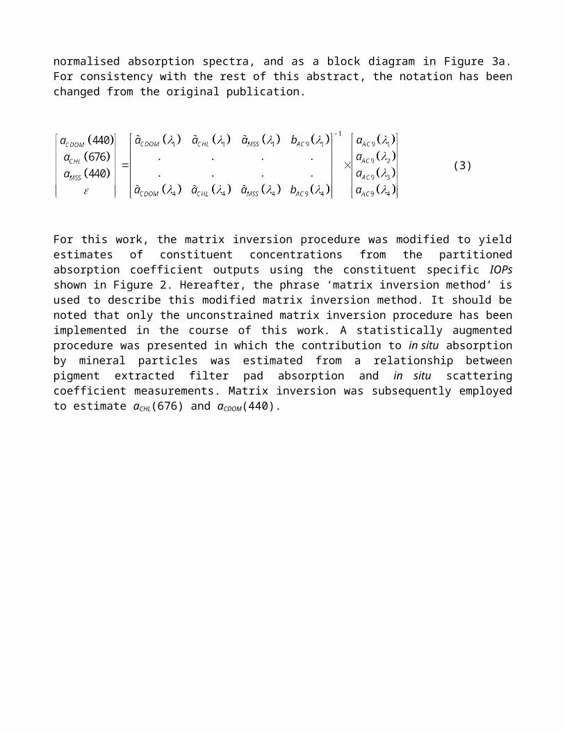
Figure 4: Semi-log plots of constituent concentration retrieval degradation in the presence of random noise in (a-c) IOPs, (d-f) sIOPs or NAS. For each maximum percentage noise (in either IOPs or sIOPs/NAS) 20 repeat tests were performed. Recall that the maximum constituent concentrations modelled were 10 mg m-3, 10 g m-3 and 1.0 m-1 for CHL, MSS and CDOM, respectively.

RESULTS

Application to field dataHaving evaluated both procedures performance using a perfect, synthetic IOP data set, both procedures were applied to an imperfect field data set. This field data set contained over 400 measurements from those stations shown in Figure 1. These stations encompassed a diverse range of coastal waters including stratified sea lochs during the phytoplankton spring bloom, significantly CDOM stained waters and highly turbid, vertically mixed estuarine waters. Constituent concentration retrievals from these field measurements, using either IOP deconvolution method, were expected to be less robust than those retrievals from synthetic IOP data. This anticipated degradation was suspected to be attributable to a combination of random and systematic measurement errors, and variability in sIOPs and NAS arising from variable constituent composition and natural particle assemblages. Figure 5 shows retrieved constituent concentrations plotted against those estimates obtained through sample analyses. Regression parameters of retrieved constituent concentrations against measured constituent concentrations are shown in Table 5. Figures 5a, 5b, 5d and 5e, show the sIOP based IOP deconvolution approach outperforming the modified matrix inversion method in the retrieval of CHL and MSS concentrations (retrieval gradients are closer to unity, offsets are lower and R2 values are slightly higher than those obtained from matrix inversion). Figures 5c and 5f show the matrix inversion method significantly outperforming the sIOP based approach in the retrieval of CDOM concentration. A possible source of the sIOP based procedures relatively poor CDOM retrieval is our current treatment of inorganic materials. Mineral particles in natural waters may be broadly considered to be of either biogenic origin, such as siliceous diatom frustules, or wholly inorganic origin, such as fine clay and silt particles. The possibility exists that the biogenic component of suspended mineral particles exhibits significantly different absorption and scattering characteristics than the wholly inorganic component. One implication of this is that treating all mineral particles as a single class of material may overestimate the absorption coefficients where the bulk of the mineral component is of biogenic origin and the sIOPs used in inversion were generated in waters containing non-biogenic mineral particles. Under such circumstances, the CDOM absorption coefficient, hence retrieved CDOM concentration, would be underestimated by the sIOP based deconvolution procedure. If conclusive evidence of significant differences in the absorption and scattering properties of these two classes of mineral particles were obtained, the in situ scattering to absorption ratio could be used as an indicator of which class of mineral particles were being encountered. This could be used to guide sIOP selection which may, in turn, improve MSS and CDOM concentration retrieval.

Method Constituent Retrieval Gradient Offset R2 RMSE

sIOP basedsIOP basedsIOP based

Matrix inversionMatrix inversionMatrix inversion

CHLMSS

CDOMCHLMSS

CDOM

1.0291.0680.7860.6610.6630.988

-0.195-0.223-0.100-0.412-1.046-0.002

0.8900.8650.5880.8600.7230.815

0.906 mg m-3

1.210 g m-3

0.198 m-1

1.649 mg m-3

2.500 g m-3

0.084 m-1

Table 5: Constituent retrieval parameters obtained by regressing retrieved constituent concentration against modelled constituent concentration for field IOP data. RMSE is used to denote ‘root-mean-square error’.

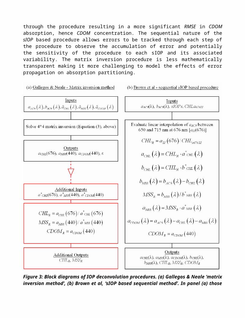
Figure 5: Plots of retrieved constituent concentration against measured constituent concentration for the UK shelf sea data set using our sIOP based IOP deconvolution technique (a-c), and the matrix inversion method (d-f). Panels (a-c) show good CHL and MSS concentration retrievals using our sIOP based deconvolution procedure with less robust CDOM retrievals. Panels (d-f) show systematic underestimation of CHL and MSS concentrations using the matrix inversion method with substantially improved CDOM retrieval.

Application to IOP depth profilesOur sIOP based IOP deconvolution procedure was applied to an AC-9 depth profile from a station in the Clyde Sea (Inchmarnock Water) and retrieved constituent concentration depth profiles are shown in Figure 6a. Pronounced vertical structure was observed in both retrieved chlorophyll and MSS concentration, with retrieved CDOM concentration (not shown) exhibiting little vertical structure and consistently low values (<0.12 m-1). Figure 6b shows hydrographic profiles of temperature and practical salinity. Figure 6c shows a strong correlation between independently measured chlorophyll fluorescence and retrieved CHL concentration. Figure 6d shows a strong correlation between the measured backscattering coefficient (at 470 nm) and retrieved MSS concentration.

Figure 6: Depth profiles from Inchmarnock Water in the Clyde Sea (occupied in April 2001) of (a) CHL and MSS concentration retrieved from AC9 measurements using our sIOP based method, (b) CTD profiles of temperature and practical salinity, (c) chlorophyll fluorescence plotted against retrieved CHL concentration, (d) bb470 plotted against retrieved MSS concentration. Panels (c) and (d) show proxy validations of retrieved constituent concentration profiles by strong correlations with independent measurements of covariant parameters. In panel (d) a small number of anomalous points are observed close to the origin of the axes. These points are from the surface 3-4 metres where a significant component of the measured MSS concentration is likely to be attributable to biogenic minerals associated with phytoplankton such as diatom frustules.

A surface CHL maximum is observed with evidence of algal material mixing downward beneath the first pycnocline (Figures 6a and 6b). Sediment accumulation is evident at 90 metres depth, possibly due to local bathymetry and tides, with resuspension or settling occuring near the seabed.

DISCUSSION AND CONCLUSIONS

A sequential, mechanistic, sIOP based IOP deconvolution procedure was developed to obtain estimates of optically significant constituent concentrations from measured in situ IOPs. Using regionally representative sIOPs from regression analyses, robust estimates of chlorophyll and MSS concentration were obtained for a diverse coastal data set. Less robust CDOM concentration retrievals were observed, possibly as a result of the propagation of errors through the sequential procedure and the prevalence of low CDOM waters sampled. Alternatively, a slightly more sophisticated model of optically significant constituents may be required to account for all of the observed variability between IOPs and the inorganic particulate component. Our procedure has been compared with a modified version of an existing matrix inversion method for partitioning absorption coefficients between constituents and comparable performance was observed using synthetic IOP data. On testing constituent concentration retrieval in the presence of random noise, each procedure exhibited distinct retrieval degradation profiles. Further investigation of retrieval degradation in the presence of both random and systematic errors should assist our understanding of the limitations of these IOP deconvolution procedures. Applying both procedures to a diverse coastal field data set suggested that the explicit use of specific absorption and scattering data in IOP inversion aided the retrieval of MSS and CHL concentrations, although robust CDOM retrievals were not observed. The potential benefit of IOP inversion was briefly illustrated by applying our sIOP-based procedure to an IOP depth profile to aid the interpretation of vertical water column structure.

REFERENCES

Astoreca R., K. Ruddick, V. Rousseau, B. Van Mol, J. Y. Parent, and C. Lancelot, 2006. Variability of the inherent and apparent optical properties in a highly turbid coastal area: Impact on the calibration of remote sensing algorithms. in Proceedings of the European Association of Remote Sensing Laboratories Proceedings 5(1): 1–17.

Barnard A. H., J. R. V. Zaneveld, and W. S. Pegau, 1999. In situ determination of the remotely sensed reflectance and the absorption coefficient: closure and inversion. Applied Optics 38: 5110–5117.

Boss E., M. S. Twardowski, and S. Herring, 2001. Shape of the particulate beam attenuation spectrum and its inversion to obtain the shape of the particulate size distribution. Applied Optics 41: 4885–4893.

Bricaud A. and D. Stramski, 1990. Spectral absorption coefficients of living phytoplankton and nonalgal biogenous matter: A comparison between the Peru upwelling area and the Sargasso Sea. Limnology & Oceanography 35: 562–582.

Bulgarelli B., G. Zibordi, and J. F. Berthon, 2003. Measured and modelled radiometric quantities in coastal waters: towards a closure,” Applied Optics 42: 5365–5381.

Chang G. C., T. D. Dickey, C. D. Mobley, E. Boss, and W. S. Pegau, 2003. Toward closure of upwelling radiance in coastal waters. Applied Optics 42: 1574–1582.

Gallegos C. L. & P. J. Neale, 2002. Partitioning spectral absorption in case 2 waters: discrimination of dissolved and particulate components. Applied Optics 41: 4220 – 4233.

Kirk J. T. O., 1994. Light and Photosynthesis in Aquatic Ecosystems, Cambridge University Press.

McKee D., A. Cunningham and S. Craig, 2003 Semi-empirical correction algorithm for AC-9 measurements in a coccolithophore bloom. Applied Optics 42: 4369 – 4374.

McKee D. and A. Cunningham, 2005 Evidence for wavelength dependence of the scattering phase function and its implication for modeling radiance transfer in shelf seas. Applied Optics 44: 126-135.

McKee D. and A. Cunningham, 2006, Identification and characterisation of two optical water types in the Irish Sea from in situ inherent optical properties and seawater constituents. Estuarine, Coastal and Shelf Science 68(1-2): 305 – 316.

Morrow J. H., W. S. Chamberlain, and D. A. Kiefer, 1989. A two-component description of spectral absorption by marine particles. Limnology & Oceanography 34: 1500–1509.

Roesler C. S., M. J. Perry, and K. L. Carder, 1989. Modelling in situ phytoplankton absorption from total absorption spectra in productive inland marine waters. Limnology & Oceanography 34: 1510–1523.

Schofield O., T. Bergmann, M. J. Oliver, A. Irwin, G. Kirkpatrick, W. P. Bissett, M. A. Moline, C. Orrico, 2004. Inversion of spectral absorption in the optically complex coastal waters of the Mid-Atlantic Bight. Journal of Geophysical Research 109: C12S04, doi:10.1029/2003JC002071.

Sullivan J. M., M. S. Twardowski, J. R. V. Zaneveld, C. M. Moore, A. H. Barnard, P. L. Donaghay and B. Rhoades, 2006. Hyperspectral temperature and salt dependencies of absorption by water and heavy water in the 400-750 nm spectral range. Applied Optics 45: 5294 – 5309.

Twardowski M. S., E. Boss, J. B. Macdonald, W. S. Pegau, A. H. Barnard, and J. R. V. Zaneveld, 2001. A model for estimating bulk refractive index from the optical backscattering ratio and the implications for understanding particle composition in case I and case II waters. J. Geophys. Res. Oceans 106: 14129–14142. Tzortziou M., J. R. Herman, C. L. Gallegos, P. J. Neale, A. Subramaniam, L. W. Harding Jr., and Z. Ahmad, 2006. Bio-optics of the Chesapeake Bay from measurements and radiative transfer closure. Estuarine, Coastal and Shelf Science 68: 348–362.

Whitmire A.L., E. Boss, T.J. Cowles and W.S. Pegau, 2007. Spectral variability of the particulate backscattering ratio. Optics Express 15(11): 7019 – 7031.

Zaneveld J. R. V., J. C. Kitchen and C. M. Moore, 1994. The scattering error correction of reflecting-tube absorption meters. Proc. SPIE 2258