ACTAUNIVERSITATIS

UPSALIENSISUPPSALA

2016

Digital Comprehensive Summaries of Uppsala Dissertationsfrom the Faculty of Science and Technology 1407

3D Time-lapse Analysis of SeismicReflection Data to Characterizethe Reservoir at the Ketzin CO2

Storage Pilot Site

FEI HUANG

ISSN 1651-6214ISBN 978-91-554-9658-6urn:nbn:se:uu:diva-301003

Dissertation presented at Uppsala University to be publicly examined in Hambergsalen,Geocentrum, Villavagen 16, Uppsala, Friday, 30 September 2016 at 10:00 for the degreeof Doctor of Philosophy. The examination will be conducted in English. Faculty examiner:Professor Andy Chadwick ( British Geological Survey).

AbstractHuang, F. 2016. 3D Time-lapse Analysis of Seismic Reflection Data to Characterize theReservoir at the Ketzin CO2 Storage Pilot Site. Digital Comprehensive Summaries of UppsalaDissertations from the Faculty of Science and Technology 1407. 73 pp. Uppsala: ActaUniversitatis Upsaliensis. ISBN 978-91-554-9658-6.

3D time-lapse seismics, also known as 4D seismics, have great potential for monitoring themigration of CO2 at underground storage sites. This thesis focuses on time-lapse analysis of 3Dseismic reflection data acquired at the Ketzin CO2 geological storage site in order to improveunderstanding of the reservoir and how CO2 migrates within it.

Four 3D seismic surveys have been acquired to date at the site, one baseline survey in 2005prior to injection, two repeat surveys in 2009 and 2012 during the injection period, and one post-injection survey in 2015. To accurately simulate time-lapse seismic signatures in the subsurface,detailed 3D seismic property models for the baseline and repeat surveys were constructed byintegrating borehole data and the 3D seismic data. Pseudo-boreholes between and beyond wellcontrol were built. A zero-offset convolution seismic modeling approach was used to generatesynthetic time-lapse seismograms. This allowed simulations to be performed quickly and limitedthe introduction of artifacts in the seismic responses.

Conventional seismic data have two limitations, uncertainty in detecting the CO2 plume inthe reservoir and limited temporal resolution. In order to overcome these limitations, complexspectral decomposition was applied to the 3D time-lapse seismic data. Monochromatic waveletphase and reflectivity amplitude components were decomposed from the 3D time-lapse seismicdata. Wavelet phase anomalies associated with the CO2 plume were observed in the time-lapsedata and verified by a series of seismic modeling studies. Tuning frequencies were determinedfrom the balanced amplitude spectra in an attempt to discriminate between pressure effectsand CO2 saturation. Quantitative assessment of the reservoir thickness and CO2 mass wereperformed.

Time-lapse analysis on the post-injection survey was carried out and the results showeda consistent tendency with the previous repeat surveys in the CO2 migration, but with adecrease in the size of the amplitude anomaly. No systematic anomalies above the caprock weredetected. Analysis of the signal to noise ratio and seismic simulations using the detailed 3Dproperty models were performed to explain the observations. Estimation of the CO2 mass anduncertainties in it were investigated using two different approaches based on different velocity-saturation models.

Keywords: storage, 3D Time-lapse (4D), Reservoir characterization, Seismic simulation,Spectral decomposition, Wavelet phase, Tuning frequency, Thin-layer thickness, Seismicmonitoring, Seismic processing, Quantitative interpretation

Fei Huang, Department of Earth Sciences, Geophysics, Villav. 16, Uppsala University,SE-75236 Uppsala, Sweden.

© Fei Huang 2016

ISSN 1651-6214ISBN 978-91-554-9658-6urn:nbn:se:uu:diva-301003 (http://urn.kb.se/resolve?urn=urn:nbn:se:uu:diva-301003)

CO2

Dedicated to my family 谨以此论文献给我的家人

List of Papers

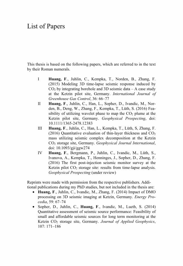
This thesis is based on the following papers, which are referred to in the text by their Roman numerals.

I Huang, F., Juhlin, C., Kempka, T., Norden, B., Zhang, F.

(2015) Modeling 3D time-lapse seismic response induced by CO2 by integrating borehole and 3D seismic data – A case study at the Ketzin pilot site, Germany. International Journal of Greenhouse Gas Control, 36: 66–77

II Huang, F., Juhlin, C., Han, L., Sopher, D., Ivandic, M., Nor-den, B., Deng, W., Zhang, F., Kempka, T., Lüth, S. (2016) Fea-sibility of utilizing wavelet phase to map the CO2 plume at the Ketzin pilot site, Germany. Geophysical Prospecting, doi: 10.1111/1365-2478.12383

III Huang, F., Juhlin, C., Han, L., Kempka, T., Lüth, S, Zhang, F. (2016) Quantitative evaluation of thin-layer thickness and CO2 mass utilizing seismic complex decomposition at the Ketzin CO2 storage site, Germany. Geophysical Journal International, doi: 10.1093/gji/ggw274

IV Huang, F., Bergmann, P., Juhlin, C., Ivandic, M., Lüth, S., Ivanova, A., Kempka, T., Henninges, J., Sopher, D., Zhang, F. (2016) The first post-injection seismic monitor survey at the Ketzin pilot CO2 storage site: results from time-lapse analysis. Geophysical Prospecting (under review)

Reprints were made with permission from the respective publishers. Addi-tional publications during my PhD studies, but not included in the thesis are:

• Huang, F., Juhlin, C., Ivandic, M., Zhang, F. (2014) Impact of DMO processing on 3D seismic imaging at Ketzin, Germany. Energy Pro-cedia, 59: 67–74

• Sopher, D., Juhlin, C., Huang, F., Ivandic, M., Lueth, S. (2014) Quantitative assessment of seismic source performance: Feasibility of small and affordable seismic sources for long term monitoring at the Ketzin CO2 storage site, Germany. Journal of Applied Geophysics, 107: 171–186

• Zhang, F., Juhlin, C., Niemi, A., Huang, F., Bensabat, J. (2015) A feasibility and efficiency study of seismic waveform inversion for time-lapse monitoring of onshore CO2 geological storage sites using reflection seismic acquisition geometries. International Journal of Greenhouse Gas Control, 48: 134–141

• Huang, F., Ivandic, M., Juhlin, C., Lüth, S., Bergmann, P., Anders-son, M., Götz, J., Ivanova, A., Zhang, F. (2016) Preliminary Seismic Time-lapse Results from the First Post-injection Survey at the Ketzin Pilot Site. 78th EAGE Conference and Exhibition, Vienna, Austria, Expanded Abstracts, Th SBT4 02

• Huang, F., Juhlin, C., Han, L., Kempka, T., Norden B., Lüth, S., Zhang, F. (2015) Application of seismic complex decomposition on thin layer detection of the CO2 plume at Ketzin, Germany. 85th SEG Annual Meeting, New Orleans, USA, Expanded Abstracts, pp. 5477–5482

• Huang, F., Juhlin, C., Kempka, T., Norden, B. (2014) Integration of Reservoir Simulation with 3D Reflection Seismic Time-lapse Data at Ketzin. 76th EAGE Conference and Exhibition, Amsterdam, Nether-lands, Expanded Abstracts, pp. 3515–3519

Contents

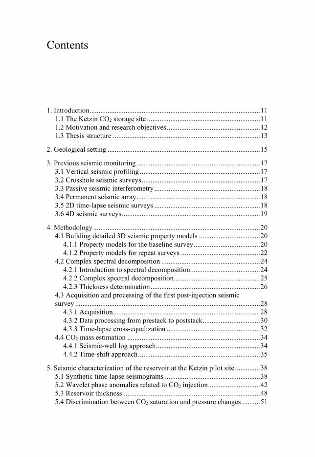
1. Introduction ............................................................................................... 11 1.1 The Ketzin CO2 storage site ............................................................... 11 1.2 Motivation and research objectives .................................................... 12 1.3 Thesis structure .................................................................................. 13

2. Geological setting ..................................................................................... 15

3. Previous seismic monitoring ..................................................................... 17 3.1 Vertical seismic profiling ................................................................... 17 3.2 Crosshole seismic surveys .................................................................. 17 3.3 Passive seismic interferometry ........................................................... 18 3.4 Permanent seismic array ..................................................................... 18 3.5 2D time-lapse seismic surveys ........................................................... 18 3.6 4D seismic surveys ............................................................................. 19

4. Methodology ............................................................................................. 20 4.1 Building detailed 3D seismic property models .................................. 20

4.1.1 Property models for the baseline survey ..................................... 20 4.1.2 Property models for repeat surveys ............................................ 22

4.2 Complex spectral decomposition ....................................................... 24 4.2.1 Introduction to spectral decomposition ....................................... 24 4.2.2 Complex spectral decomposition ................................................ 25 4.2.3 Thickness determination ............................................................. 26

4.3 Acquisition and processing of the first post-injection seismic survey ....................................................................................................... 28

4.3.1 Acquisition .................................................................................. 28 4.3.2 Data processing from prestack to poststack ................................ 30 4.3.3 Time-lapse cross-equalization .................................................... 32

4.4 CO2 mass estimation .......................................................................... 34 4.4.1 Seismic-well log approach .......................................................... 34 4.4.2 Time-shift approach .................................................................... 35

5. Seismic characterization of the reservoir at the Ketzin pilot site .............. 38 5.1 Synthetic time-lapse seismograms ..................................................... 38 5.2 Wavelet phase anomalies related to CO2 injection ............................. 42 5.3 Reservoir thickness ............................................................................ 48 5.4 Discrimination between CO2 saturation and pressure changes .......... 51

5.5 Time-lapse analysis of the first post-injection survey ........................ 53 5.6 Quantitative assessment of the CO2 mass .......................................... 56

6. Conclusions and outlook ........................................................................... 61 6.1 Conclusions ........................................................................................ 61 6.2 Outlook ............................................................................................... 63

7. Summary in Swedish ................................................................................ 64

Acknowledgements ....................................................................................... 68

References ..................................................................................................... 70

Abbreviations

1D 2D 3D 4D AVO CCS CDP CO2 CO2SINK CWT CSD DAS DFT FD FX Hz km kt m mD MPa ms Mt NMO NRMS PNG RMS s STFT S/N TLD

One-dimensional Two-dimensional Three-dimensional Four-dimensional Amplitude versus offset Carbon capture and storage Common depth point Carbon dioxide CO2 Storage by Injection into a Natural saline aquiferat Ketzin Continuous wavelet transform Complex spectral decomposition Distributed Acoustic Sensing Discrete Fourier transform Finite difference Frequency-space Hertz Kilometer Kiloton Meter Millidarcy Mega-Pascal Millisecond Megaton Normal moveout Normalized root-mean-square Pulsed neutron-gamma Root-mean-square Second Short-time Fourier transform Signal-to-noise ratio Time-lapse differences

TWT VSP WNW WVD

Two-way traveltime Vertical seismic profile West-northwest Wigner-Ville distribution

11

1. Introduction

1.1 The Ketzin CO2 storage site NASA’s Earth Observatory indicates that the average global temperature on Earth has increased by 0.6 to 0.9 degrees Celsius since 1906. A doubled rate of warming has been observed over the past 50 years. Consequently, the average global sea level has risen by 0.19 m since then (IPCC, 2013). Car-bon Dioxide (CO2) is considered as the most significant greenhouse gas that primarily leads to global warming. Human activities like burning fossil fuels contributes to the rise of CO2 concentration in the atmosphere. If temperature continues to go up, the Earth might not remain habitable for some fauna and flora as well as for humans. In 2010, world leaders signed the Cancun Agreements and agreed to commit government to avoid the average global temperature increase above two degrees Celsius.

Carbon capture and storage (CCS) has been considered as a key technolo-gy to achieve this objective given that it is impossible to completely stop burning fossil fuels in the foreseeable future. CCS is the process that cap-tures CO2 emissions from fossil fuel based power generation or industrial facilities and safely stores them underground for a long time. In 2015, there were 15 large-scale CCS projects with CO2 capture of up to 28 Mt per year and 7 more projects were in the execution stage (Global CCS Institute, 2015). In Europe, there are two active large-scale CCS projects: the Sleipner project in the North Sea (Kongsjorden et al., 1998) and the Snøhvit project in the Barents Sea (Hansen et al., 2013).

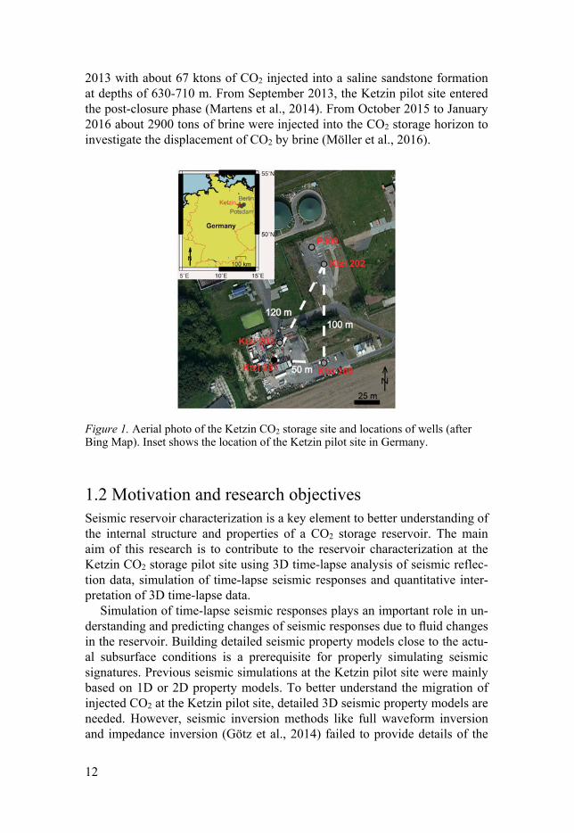
The first European on-shore CO2 storage project, the CO2SINK (CO2 Storage by Injection into a Natural saline aquifer at Ketzin) project (Förster et al. 2006), financed by the European Commission, was initiated in 2004 with the aim to expand the experience in monitoring CO2 underground stor-age and to provide confidence for future European onshore CCS projects. The selected test site was located in Ketzin, a small town 25 km west of Ber-lin, Germany (Figure 1). The drilling of one injection well (Ktzi 201) and two observation wells (Ktzi 200 and Ktzi 202), down to a depth of approxi-mately 800 m, was completed in 2007. The injection of CO2 started in June 2008. In 2011 and 2012, two additional observation wells, P300 which is 180 m above the storage formation, and Ktzi 203 which was drilled down to a depth of 700 m were completed. The injection of CO2 ended on August 29,

12

2013 with about 67 ktons of CO2 injected into a saline sandstone formation at depths of 630-710 m. From September 2013, the Ketzin pilot site entered the post-closure phase (Martens et al., 2014). From October 2015 to January 2016 about 2900 tons of brine were injected into the CO2 storage horizon to investigate the displacement of CO2 by brine (Möller et al., 2016).

Figure 1. Aerial photo of the Ketzin CO2 storage site and locations of wells (after Bing Map). Inset shows the location of the Ketzin pilot site in Germany.

1.2 Motivation and research objectives Seismic reservoir characterization is a key element to better understanding of the internal structure and properties of a CO2 storage reservoir. The main aim of this research is to contribute to the reservoir characterization at the Ketzin CO2 storage pilot site using 3D time-lapse analysis of seismic reflec-tion data, simulation of time-lapse seismic responses and quantitative inter-pretation of 3D time-lapse data.

Simulation of time-lapse seismic responses plays an important role in un-derstanding and predicting changes of seismic responses due to fluid changes in the reservoir. Building detailed seismic property models close to the actu-al subsurface conditions is a prerequisite for properly simulating seismic signatures. Previous seismic simulations at the Ketzin pilot site were mainly based on 1D or 2D property models. To better understand the migration of injected CO2 at the Ketzin pilot site, detailed 3D seismic property models are needed. However, seismic inversion methods like full waveform inversion and impedance inversion (Götz et al., 2014) failed to provide details of the

13

reservoir due to the relatively short offsets (maximum c. 1000 m) for 3D seismic surveys and the presence of a thin high-velocity anhydrite layer (about 5500 m/s) situated about 80 meters above the reservoir.

Several limitations also exist in quantitative interpretation of 3D time-lapse data. First, the conventional band-limited seismic cannot resolve thin layers (e.g. paleochannels or sandstone channels) which are common in CO2 storage. Second, uncertainty exists in identifying the seismic anomaly due to injected CO2. For instance, time-lapse noise and pressure effects may gener-ate similar anomalies as CO2 related anomalies. Third, quantitative analysis of the CO2 plume is susceptible to errors in the reservoir parameters because of a limited number of boreholes, reservoir heterogeneity and upscaling er-rors.

Guided by these challenges, the research in this thesis has the following objectives: 1. To efficiently integrate the existing borehole data and the 3D seismic

data to build detailed 3D seismic property models for seismic simulation at the Ketzin pilot site.

2. To investigate the feasibility of utilizing wavelet phase changes related to the CO2 plume to reduce the uncertainty in monitoring the CO2 distri-bution.

3. To determine tuning frequency to quantitatively assess the thickness and mass of the gaseous CO2 and to attempt the discrimination between the pressure effects and CO2 saturation.

4. To evaluate the recent development of the CO2 plume in the post-closure phase and to estimate the CO2 mass using two different models (patchy and non-patchy saturation models).

1.3 Thesis structure This thesis consists of seven chapters and four accompanying papers. Chap-ter 1 gives a general introduction to the Ketzin CO2 storage pilot site togeth-er with the motivation and research objectives. Chapter 2 provides the geo-logical setting of the Ketzin pilot site. In Chapter 3 a brief overview is given of the seismic methods previously used at the site. Chapter 4 includes the research methodology used in this thesis. Chapter 5 discusses the time-lapse results at the Ketzin pilot site in detail using the methods described in Chap-ter 4. Chapter 6 concludes the research achievements in this thesis. Chapter 7 is the summary in Swedish. Paper I: To model time-lapse seismic signatures at the Ketzin pilot site, de-tailed 3D seismic property models for the baseline and repeat surveys were efficiently built by integrating borehole data and 3D seismic data. Seismic velocity and density after CO2 injection were calculated using CO2 parame-

14

ters from the history-matched dynamic flow simulations. A simple convolu-tion approach was used to produce synthetic zero-offset time-lapse seismic responses with the aim of saving computational cost and not introducing processing artifacts. Close agreement between the synthetic and real data at the corresponding time shows that the 3D property models were adequate to simulate the time-lapse responses at the Ketzin CO2 storage pilot site. Paper II: In this work, a feasibility study of utilizing wavelet phase compo-nents extracted by complex spectral decomposition to monitor the CO2 plume at the Ketzin site was conducted. To provide better understanding of the phase changes related to the injected CO2, analysis of acous-tic/viscoacoustic simulations were implemented. Distinct phase features correlated with the sandstone channels, CO2 plume and ambient noise were identified, suggesting that it is practical to combine wavelet phase infor-mation with seismic amplitude to decrease the uncertainty in detecting CO2 plume in the reservoir. Paper III: This paper presents the case study from the Ketzin site in which frequency characteristics of thin layers were obtained from the 3D time-lapse seismic data using complex spectral decomposition. The extracted reflectivity amplitude sections show improved temporal resolution and more stratigraphic details. The thickness of the reservoir sandstone and gaseous CO2 determined using the extracted tuning frequency is consistent with the well logging data. An attempt to distinguish between the saturation and pres-sure anomalies reveals that the majority of the amplitude anomaly is related to CO2 saturation. The CO2 mass estimated using the saturation-related anomaly agrees with the actual amount of the injected CO2 but with some discrepancy. Paper IV: To evaluate the recent development of the CO2 plume, a third 3D repeat seismic survey, serving as the first post-injection survey, was con-ducted in 2015 in the post-closure phase of the project at the Ketzin site. This study presents the processing and time-lapse analysis results from the first post-injection survey. The CO2 plume migrates towards the WNW in the up-dip direction, consistent with the previous surveys. No anomalies above the caprock are detected. Compared with the amplitude anomaly in the reservoir at the time of the second repeat survey, a decrease in the range and intensity is observed. A more significant decrease of the amplitude anomaly occurs east and south of the injection site. Seismic simulations re-veal a dynamic balance between the newly injected CO2 of 6 kt and the CO2 being dissolved and diffused. Due to the significant uncertainty that exists in the CO2 mass calculation, both patchy and non-patchy saturation models were investigated.

15

2. Geological setting

Ketzin is situated in the Northeast German Basin, which is a subbasin of the Southern Permian Basin in Europe (Ziegler, 1990). Initial rifting in the early Permian together with the following subsidence and the deposition of Permi-an clastic sediments and Upper Permian Zechstein salt contributed to the evolution of the basin. Since the Triassic times, salt tectonics at around 1500-2000 m depth led to the deformation of the overburden and formed anticlines and synclines (Kossow et al., 2000). The Ketzin pilot site is lying on the southern flank of an anticline dipping 15 degrees, which is a part of the west-southeast to east-northeast Roskow-Ketzin double anticline (Förster et al., 2006).

Almost pure CO2 was injected into the 80 m thick Triassic Stuttgart For-mation at depths of 630-710 m (Figure 2). Sandy channel-facies rocks alter-nating with muddy, flood-plain-facies rocks comprise the lithologically het-erogeneous Stuttgart Formation. The thickness of the sandstone intervals may be up to several tens of meters where subchannels are stacked together. These well-sorted and fine- medium grained sandstones are well sorted and weakly cemented by silicates and clay, and sometimes by anhydrite or halite as well (Norden et al., 2010). Core analysis on reservoir-rock samples exhib-it varying porosity (from 5 to 35%) and brine permeability (from 0.02 to 5000 mD) (Norden et al., 2010). The lower part of the Stuttgart Formation consists of overbank sediments such as silty sandstones and siltstones char-acterized by their thickness and mineralogical composition. The upper sand-stone layers of the Stuttgart Formation are 9-20 thick channel deposits with good reservoir quality. Temperature and pressure measured at the injection horizon are in a range of 34 to 38 ºC (Förster et al., 2006) and 6.21 to 6.47 MPa (Kazemeini, 2009), respectively.

16

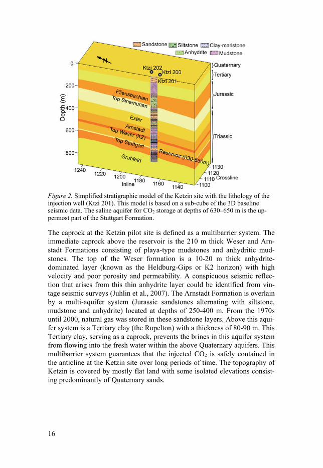
Figure 2. Simplified stratigraphic model of the Ketzin site with the lithology of the injection well (Ktzi 201). This model is based on a sub-cube of the 3D baseline seismic data. The saline aquifer for CO2 storage at depths of 630–650 m is the up-permost part of the Stuttgart Formation.

The caprock at the Ketzin pilot site is defined as a multibarrier system. The immediate caprock above the reservoir is the 210 m thick Weser and Arn-stadt Formations consisting of playa-type mudstones and anhydritic mud-stones. The top of the Weser formation is a 10-20 m thick anhydrite-dominated layer (known as the Heldburg-Gips or K2 horizon) with high velocity and poor porosity and permeability. A conspicuous seismic reflec-tion that arises from this thin anhydrite layer could be identified from vin-tage seismic surveys (Juhlin et al., 2007). The Arnstadt Formation is overlain by a multi-aquifer system (Jurassic sandstones alternating with siltstone, mudstone and anhydrite) located at depths of 250-400 m. From the 1970s until 2000, natural gas was stored in these sandstone layers. Above this aqui-fer system is a Tertiary clay (the Rupelton) with a thickness of 80-90 m. This Tertiary clay, serving as a caprock, prevents the brines in this aquifer system from flowing into the fresh water within the above Quaternary aquifers. This multibarrier system guarantees that the injected CO2 is safely contained in the anticline at the Ketzin site over long periods of time. The topography of Ketzin is covered by mostly flat land with some isolated elevations consist-ing predominantly of Quaternary sands.

17

3. Previous seismic monitoring

A wide range of geophysical methods (Martens et al., 2014; Bergmann et al., 2016), such as well logging, seismic and electro-magnetic techniques have been applied to the Ketzin pilot site in order to map the geologic structure and the distribution of the injected CO2 plume. Other methods like geochem-ical (Zimmer et al., 2011) and geodetic (Lubitz and Motagh, 2013) meas-urements were also used to implement further monitoring. A brief overview of the seismic methods previously used in this project is given below.

3.1 Vertical seismic profiling Vertical seismic profiling (VSP) is a seismic method, which records seismic waves generated by a source with receivers deployed in a borehole. A VSP survey is implemented to correlate between surface seismic data and subsur-face stratigraphy since it can provide higher resolution subsurface images within the vicinity of the wellbore. At the Ketzin site, swept source (VIB-SIST-1000/3000 with a hydraulic driven concrete breaking hammer) was used to acquire time-lapse zero-offset VSP and offset-VSP data (Yang et al., 2010). Baseline VSP data were recorded in 2007 prior to the CO2 injection, while one repeat zero-offset VSP survey in 2011 and two repeat offset-VSP surveys in 2009/2011 were performed. The results show that in comparison with surface seismics, the imaged reflections have higher vertical and lateral resolutions.

Fibre-optic Distributed Acoustic Sensing (DAS) is a relatively new tool with the use of optical fiber cable for measuring strain changes of the fiber within acoustic frequencies. DAS-VSP data were also tested at the Ketzin site and showed promising image quality (Daley et al., 2013).

3.2 Crosshole seismic surveys In cross-hole seismic surveys, seismic waves generated in a borehole are acquired by receivers in other boreholes. At the Ketzin site, a time-distributed VIBSIST piezoelectric borehole source was used in the Ktzi 200

18

borehole while 12 hydrophones were placed at depths of 464-726 m in the Ktzi 202 borehole. From May 2008 to August 2008, one baseline and two repeat surveys were performed (Zhang et al., 2012). At the times of the two repeat surveys, approximately 660 and 1750 tons of CO2 had been injected into the saline aquifer, respectively. However, no clear observable time-lapse changes were recognized since a very small amount of CO2 had migrated through the imaging plane, but not yet arrived at Ktzi 202.

3.3 Passive seismic interferometry Seismic interferometry is a technique that cross-correlates seismic signals observed at different locations in order to reconstruct useful reflection re-sponses from subsurface layers. Since seismic interferometry uses ambient seismic noise instead of an active seismic source, it is a relatively cost-effective and environmentally friendly methodology. Ambient noise data were measured at the Ketzin pilot site in February 2011 (Xu et al., 2012), August 2013 (Zhang et al., 2015) and October 2015. Compared with passive and active stacked sections, similar seismic reflections, especially from the shallower subsurface, can be identified.

3.4 Permanent seismic array Permanent seismic array is a seismic monitoring system using permanently installed receivers. To record both active and passive seismic data from Ketzin, multicomponent geophones/hydrophones were permanently placed at 50 m depth and at the surface (Arts et al., 2011). The continuously record-ing passive seismic data were used for monitoring the injection-induced seismic activity and ambient-noise seismic interferometry (Boullenger et al., 2014). This system maximizes the repeatability of the recording conditions. Analysis of the buried data shows an increased frequency bandwidth up to 300 Hz (Arts et al., 2011). Due to the absence of baseline data before CO2 injection, further investigation is required to verify the potential of monitor-ing CO2 migration.

3.5 2D time-lapse seismic surveys 2D time-lapse seismic data were acquired along seven 2D lines with a radial acquisition geometry around the injection well Ktzi 201. Seismic data along all the 2D lines with receiver station spacing of 24 m were acquired simulta-neously by activating the VIBSIST source. In this way, sparse 3D time-lapse seismic images were obtained. To increase the fold around the injection site,

19

two shorter receiver lines were deployed in the vicinity of the site. The base-line survey was conducted in November 2005 while two repeat surveys were conducted in September 2009 and February 2011 after the CO2 injection of 22 and 45 kt, respectively. In comparison with the results from the 3D seis-mic surveys, the CO2-induced amplitude anomalies in the sparse 3D images exhibit similar migration trends of the CO2 plume, but with a reduced extent and intensity and higher levels of noise (Ivandic et al., 2012). This may be due to the uneven distribution of the acquisition geometry.

3.6 4D seismic surveys Compared with the other seismic surveys, wide-ranging coverage of the subsurface and higher lateral resolution are the advantages of 3D seismic surveys. At the Ketzin pilot site, there have been three full 3D seismic sur-veys from 2005 to 2012.

The baseline 3D survey was acquired in the autumn of 2005 prior to the start of the CO2 injection in order to image the structural geometry of the reservoir (Juhlin et al., 2007). To monitor the movement of the CO2 plume, two repeat 3D surveys were conducted in the autumns of 2009 and 2012, after injection of approximately 22-25 and 61 kt of CO2, respectively (Ivanova et al. 2012, Ivandic et al. 2015). The same acquisition template scheme was used in all the 3D seismic surveys. The baseline survey area includes 41 templates (~ 14 km2) located around the injection site while the two repeat survey areas include 20 (~ 7 km2) and 31 (~ 10 km2) templates, respectively. The same processing steps (except for static corrections) were applied to the baseline (Juhlin et al., 2007) and two repeat surveys (Ivanova et al. 2012, Ivandic et al. 2015) for improving time-lapse seismic repeatability. Results from the 4D seismic surveys show that the seismic amplitude anomaly caused by the injected CO2 plume was concentrated around the injection well with a predominantly westward propagation (Ivanova et al. 2012, Ivandic et al. 2015). CO2 mass estimates at the times of the two repeat surveys were consistent with the actual injected mass of CO2 but with considerable uncertainty. No systematic amplitude anomalies were detected within the overburden.

20

4. Methodology

This section summarizes the methods applied to 3D time-lapse seismic data in order to characterize the reservoir at the Ketzin pilot site.

4.1 Building detailed 3D seismic property models Compared with 3D seismic data, which contain information over a large area and have limited vertical resolution, well-log data provide information with higher vertical resolution, but only at the well location. By integrating bore-hole data and 3D seismic data, detailed seismic property models within the target area encompassing the CO2 migration can be constructed (Huang et al., 2015).

4.1.1 Property models for the baseline survey Considering the highly heterogeneous reservoir at the Ketzin site, it is a re-quirement to build pseudo-boreholes between and beyond well control to constraint the interpolation, when building seismic property models. Three wells (Ktzi 200, Ktzi 201 and Ktzi 202) are available for building baseline property models, the other two wells (P300 and Ktzi 203) were drilled and measured after CO2 injection. Varying quality of well-log data can be found in the three available wells because of borehole breakouts, missing data and noise due to drill mud management activities (Norden and Frykman, 2013). For instance, when comparing synthetic and real traces, the Ktzi 201 well shows the best cross-correlation coefficient within the reservoir and immedi-ate caprock formations, whereas the Ktzi 202 well shows the best cross-correlation coefficient above the caprock. Therefore an idealized borehole, combining data from both of these wells was simulated and used as a refer-ence for the other pseudo-boreholes.

The first step was to construct a 10-layer depth model derived from seis-mic horizons corresponding to the top of the Pliensbachian, Sinemurian, Exter, Arnstadt, Weser, Stuttgart and Grabfeld formations, as well as the base of the K2 and reservoir horizons. The Quaternary and Tertiary for-mations were merged into one layer due to the lack of sonic borehole data and the relatively poor near surface image in the seismic data. Assuming almost constant facies in each layer, log data within one layer can be trans-

21

ferred from the existing boreholes to the pseudo-boreholes by performing linear interpolation. In order to build the idealized borehole the density and sonic data were used from the Ktzi 201 well, with the exception of the data from the reservoir and immediate caprock formations, where data from the Ktzi 202 well was used. In this way, the idealized borehole data for the well Ktzi 202 was constructed. The well data at every 5th CDP were then interpo-lated using the horizons to define the variation of thickness away from the idealized borehole. A good match between the original and transferred logs for the Ktzi 200 well (Figure 3) verifies the effectiveness of this method.

Figure 3. Comparison of the well Ktzi 200 (red) and the corresponding pseudo-borehole (blue). Left two columns: density logs (RHOB); right two columns: sonic logs (DT). The green lines represent the density and sonic logs of the idealized bore-hole for the well Ktzi 202. Red and blue lines represent the original and transferred logs for the well Ktzi 200, respectively. Dotted lines mark the correlation of hori-zons in the wells.

Due to the lack of data in the very shallow part of the well a time shift exists between the synthetic seismogram generated from the pseudo-borehole and the composite seismogram, generated by averaging the real traces within +/-1 CDP of the corresponding location. The prominent and continuous K2 horizon was set as the reference horizon to perform calibration for the sonic logs of the pseudo-boreholes. The synthetic trace was shifted so that the strong K2 reflection matched the K2 reflection in the surface seismic data. The main reflections present in both the synthetic and real traces were set as control points. Like calibration using check shots in a VSP survey, the syn-thetic trace was matched to the corresponding composite trace by performing a spline interpolation between two control points. Consequently, the cali-

22

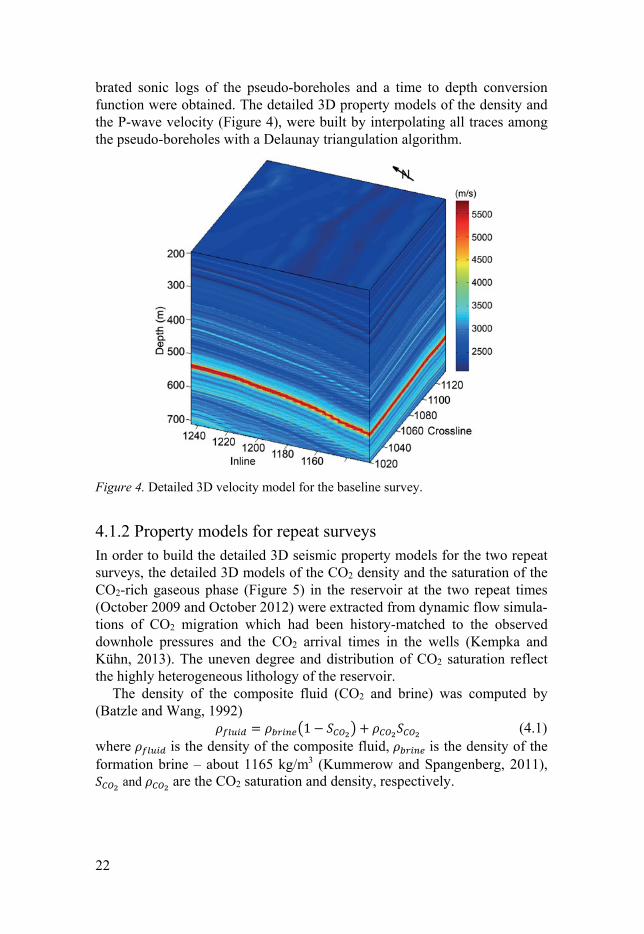
brated sonic logs of the pseudo-boreholes and a time to depth conversion function were obtained. The detailed 3D property models of the density and the P-wave velocity (Figure 4), were built by interpolating all traces among the pseudo-boreholes with a Delaunay triangulation algorithm.

Figure 4. Detailed 3D velocity model for the baseline survey.

4.1.2 Property models for repeat surveys In order to build the detailed 3D seismic property models for the two repeat surveys, the detailed 3D models of the CO2 density and the saturation of the CO2-rich gaseous phase (Figure 5) in the reservoir at the two repeat times (October 2009 and October 2012) were extracted from dynamic flow simula-tions of CO2 migration which had been history-matched to the observed downhole pressures and the CO2 arrival times in the wells (Kempka and Kühn, 2013). The uneven degree and distribution of CO2 saturation reflect the highly heterogeneous lithology of the reservoir.

The density of the composite fluid (CO2 and brine) was computed by (Batzle and Wang, 1992)

= 1 − + (4.1) where is the density of the composite fluid, is the density of the formation brine – about 1165 kg/m3 (Kummerow and Spangenberg, 2011),

and are the CO2 saturation and density, respectively.

23

Figure 5. Saturation of CO2-rich gaseous phase at the first repeat time (left) and the second repeat time (right).

Considering that the reservoir rock at the Ketzin site mainly consists of clay-rich arkosic sandstone (Norden et al., 2010) and the dry-out zone is only near the injection well, a more reasonable assumption is that CO2 saturation is related to the effective porosity rather than total porosity. Therefore, the equation for estimating the density of the rock in the brine/composite fluid can be written as = ∅ + ∅ − ∅ + (1 − ∅ ) , (4.1) where ∅ and ∅ represent the effective and total porosities, which were derived from porosity data in the three wells (Norden et al., 2010), and represents the matrix density. can be calculated from the measured bulk density of the rock ( ) which is fully saturated with brine using equation (4.2) (Ivanova et al., 2013b)

= ∅∅ . (4.2)

Petrophysical experiments on reservoir rock were conducted at the Ketzin site (Kummerow and Spangenberg, 2011; Ivanova et al., 2013b) and showed a near linear velocity-saturation relationship which follows = −0.46 , (4.3)

where is the P-wave velocity before CO2 injection and Δv is change in P-wave velocity. This velocity-saturation relationship was used to estimate P-wave velocity after CO2 injection. Given that a very minor change (2%) in S-wave velocity was observed and that this study focuses on changes in the amplitude of P-wave reflectivity, changes in the S-wave velocity were ne-glected.

24

4.2 Complex spectral decomposition This section first gives a brief introduction to spectral decomposition tech-niques. The theory and application of complex spectral decomposition (CSD) which is used in this thesis is then discussed.

4.2.1 Introduction to spectral decomposition Seismic signals which are non-stationary contain a lot of useful frequency-dependent information. However, conventional seismic methods cannot ex-tract this frequency-dependent information. Like a prism splitting light into different colors, spectral decomposition is a powerful and advanced tool, to decompose a non-stationary seismic signal into its constituent frequency components. It enables the interpreter to observe amplitude and phase tuned to specific wavelengths. This decomposed frequency information is useful for seismic imaging and interpretation, like mapping the temporal thickness of thin beds and detecting hydrocarbon reservoirs.

The methodology and applications of spectral decomposition have devel-oped quickly in the past few decades. The discrete Fourier transform (DFT) is one of the most fundamental and widely used mathematical methods. It transforms a discrete-time signal into a discrete set of phase and frequency pairs. However, the DFT is not sensitive to time-varying changes in frequen-cy. To gain understanding of variations in frequency content with time the short-time Fourier transform (STFT) method, which uses a constant time window for the Fourier transform was proposed. A special case of STFT is Gabor transform which uses the Gabor function for the windowing (Gabor, 1946a). The constant length of the window fixes the time and frequency resolutions for all the components and may also lead to truncation errors (Hall, 2006). The continuous wavelet transform (CWT) (Haar, 1910) is a potential solution for this limitation. It divides the signal into wavelets with varying scales and translations. The length of the window changes with the signal frequency. Therefore, acceptable temporal resolution for high fre-quency components and acceptable frequency resolution for low frequency components can be obtained (Kumar and Foufoula-Georgiou, 1997). To solve different problems, a range of other time-frequency decomposition methods like matching pursuit, Wigner-Ville distribution (WVD), S trans-form and the synchrosqueezing transform have also been developed (Tary et al., 2014).

Complex spectral decomposition (CSD) (Bonar and Sacchi, 2010) utilizes inversion strategies to decompose the seismic signal into a series of complex wavelets with distinct frequencies and phases. In comparison with the con-ventional spectral decomposition methods, the complex time–frequency spectrum generated by CSD is less constrained by the Heisenberg-Gabor

25

uncertainty principle (Gabor, 1946b) and contains wavelet phase infor-mation.

4.2.2 Complex spectral decomposition A seismic trace containing multiple wavelets can be regarded as the summa-tion of convolutions of several wavelets with the corresponding reflectivity sequences (Bonar et al., 2010). Considering a realistic seismic trace con-taminated with noise, the seismic trace can be represented by

= ∑ ∗ + (4.1) where is the number of wavelets, ∗ denotes convolution, represents the th wavelet with dominant frequency f in the wavelet library, represents

the corresponding reflectivity series and represents noise in the trace. Using convolution matrices, equation 4.1 can be equally written as

= ( ⋯ ) ⋮ + (4.2)

where is the convolution matrix of the wavelet . The simplified expression of equation 4.2 is = + (4.3)

where is the convolution matrix of the wavelet library and is the corre-sponding reflectivity series.

In order to provide the phase information, the real-valued wavelet library can be transformed to the complex wavelet library by performing the Hilbert transform. Using zero-phase wavelets in the wavelet library, the phase in-formation of the seismic trace can consequently be maintained in the com-plex reflectivity series (Bonar and Sacchi, 2010; Han et al., 2015; Liu et al., 2015).

To determine the complex time–frequency spectrum by solving equa-tion 4.3 is an underdetermined inverse problem. By utilizing the L2-norm to measure data misfit and the L1-norm to improve sparsity, the cost function can be constructed as

= ‖ − ‖ + ‖ ‖ , > 0 (4.4)

where λ is the regularization parameter that controls the sparsity of solutions. A comparison of the time-frequency spectra obtained by the Gabor trans-

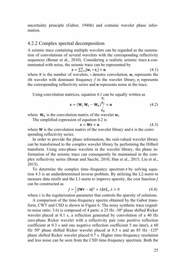
form, CWT and CSD is shown in Figure 6. The noisy synthetic trace (signal-to-noise ratio: 3.6) is composed of 4 parts: a 25 Hz -30º phase shifted Ricker wavelet placed at 0.1 s, a reflection generated by convolution of a 40 Hz zero-phase Ricker wavelet with a reflectivity pair (one positive reflection coefficient at 0.3 s and one negative reflection coefficient 5 ms later), a 60 Hz 50º phase shifted Ricker wavelet placed at 0.5 s and an 85 Hz -125º phase shifted Ricker wavelet placed 0.7 s. Higher time-frequency resolution and less noise can be seen from the CSD time-frequency spectrum. Both the

26

frequency and phase information of the seismic traces are correctly identi-fied. The reflectivity pair of the second reflection is also clearly recogniza-ble.

Figure 6. Comparison of the time-frequency spectra obtained by Gabor transform, CWT and CSD. (a) Synthetic trace contaminated with random noise, (b) Gabor spectrum, (c) CWT spectrum, (d) CSD reflectivity spectrum, (e) CSD wavelet phase spectrum. Inset shows a close-up image of the second reflection.

4.2.3 Thickness determination The thickness of the main-reservoir sandstone in the upper part of the Stuttgart Formation at the Ketzin site is in the range of 9-20 m (Förster et al., 2010), which is generally below 1/4 of the dominant wavelength. Therefore, conventional band-limited seismic reflection data have difficulties in deter-mining the thickness of the thin layers. Partyka et al. (1999) presented that the relationship between two-way temporal thickness t of the layer and the period of the amplitude spectrum in the frequency domain Pf follows t=1/Pf=1/2f, where f is the first tuning frequency. The amplitude spectrum of the thin layer can be obtained by transforming the seismic reflection from the thin layer over a given time window. In practice, truncation errors may be introduced after windowing due to incomplete separation from the adja-cent reflections (Hall, 2006), especially for closely placed reflections. With the aim to decrease the truncation errors, the reflectivity amplitude data which were obtained using CSD and have higher resolution than the conven-tional seismic reflection data are used to determine the tuning frequency. In this way, the zone of interest can be more easily and correctly delineated. The discrete-frequency reflectivity amplitude data within the delineated zone (the zone of the reservoir layer) are converted into the frequency domain. After multiplying the corresponding amplitude spectrum of the wavelet in the complex wavelet library and summing all the monochromatic amplitude spectra, the amplitude spectrum of the thin layer is generated. To extract thin-bed interference which can be used to determine tuning frequency, the source wavelet overprint needs to be removed from the amplitude spectrum

27

(Partyka et al., 1999). In order to do this, the amplitude spectrum is balanced by the extracted wavelet.

To verify the effectiveness of this method, a synthetic time-lapse case was tested. The velocity and density of the baseline model (Figure 7a) was de-rived from the log data from the Ktzi 201 well (Norden et al., 2010). The second layer represents the reservoir sandstone. The tuning frequency related to the second layer was determined from the amplitude spectrum after apply-ing CSD to the synthetic baseline data. Figures 7b and 7c show that the de-termined tuning frequency and temporal thickness are consistent with theo-retical values. CO2 was injected into the second layer which generates a new layer with a lower velocity (Figure 8a). To calculate the temporal thickness of the CO2 plume, the tuning frequency was determined from the amplitude spectrum after applying CSD to the synthetic time-lapse amplitude differ-ence. Figures 8b and 8c show reasonable agreement with the theoretical val-ues, but with increased error due to the impact of the base of the reservoir. Note that the location of the first tuning frequency corresponds to the first trough of the balanced amplitude spectrum for the reservoir top and base with the same polarity (Figure 7b), whereas the location of the first tuning frequency corresponds to the first peak of the balanced amplitude spectrum for the reservoir top and base with the opposite polarity (Figure 8b). For the seismic data from the Ketzin pilot site, the polarity of the reservoir top and base is undetermined because of the reservoir heterogeneity. To solve this problem, both the first peaks of the balanced amplitude spectrum and the balanced amplitude spectrum multiplied by -1 were determined. The mini-mum between these two first peaks corresponds to the proper first tuning frequency.

Figure 7. (a) Velocity model of baseline, (b) amplitude spectrum of trace 92 and the determined tuning frequency (green triangle), (c) comparison of theoretical (red) and determined (blue) temporal thickness.

28

Figure 8. (a) Velocity model of repeat, (b) amplitude spectrum of trace 92 and the determined tuning frequency (green triangle), (c) comparison of theoretical (red) and determined (blue) temporal thickness.

4.3 Acquisition and processing of the first post-injection seismic survey In order to track the migration of the injected CO2 in the post-closure phase at the Ketzin pilot site, the third 3D repeat seismic survey, also known as the first post-injection survey, was acquired in autumn 2015. This section pre-sents the acquisition and processing of the first post-injection seismic survey.

4.3.1 Acquisition The same template-based acquisition scheme (Figure 9), as for the previous 3D seismic surveys, was employed in the first post-injection seismic survey, with the aim of keeping the utmost repeatability of receiver coupling and positioning between the baseline and repeat surveys. The template system was numbered with an origin in the lower left hand corner of the survey area. Each template has the same acquisition geometry (Juhlin et al., 2007). One template consisted of five receiver lines with twelve perpendicular source lines. Receiver line spacing was 96 m and station spacing was 24 m. The first post-injection survey includes 33 templates, covering an area of approx-imately 11 km2. Two new templates (Templates 5.0 and 6.0) were added in the westernmost part in order to expand the baseline survey into an area where the CO2 plume is anticipated to later propagate. Templates with the same first number (e.g., Templates 6:1, 6:2, 6:3 etc.) belong to the same swath. The acquisition parameters are summarized in Table 4.1.

29

Figure 9. Template-based acquisition scheme used in the first post-injection (third repeat) 3D survey. Magenta lines outline the survey area. Green isolines denote the topography of the storage formation. Red and yellow dots represent the locations of the injection well (Ktzi 201) and three observation wells (Ktzi 200, 202, and 203), respectively.

Table 4.1 Template acquisition parameters.

Parameter Value

Receiver line spacing/number per template 96 m/5Receiver station spacing/channels per template 24 m/48Source line spacing/number per template 48 m/12Source point spacing 24 m or 72 mCDP bin size 12 m × 12 mNominal fold 25Geophones 28 Hz singleSampling rate 1 msRecord length 3 sSource 240 kg accel. weight drop, 8 hits per

shot pointAcquisition unit Sercel 428 XL

Acquisition of the first post-injection survey, using an accelerated weight drop began in template 9:5 on September 2, 2015 and proceeded through the survey area in a snake-like manner. Typically 8 hits were stacked for each shot point to obtain better signal to noise ratio. For points in noisy or wet conditions the number of hits was increased. When moving receiver lines from one template to another template within a swath (e.g. Templates 8:2, 8.3), half of the receiver stations remained. Half of the source points over-lapped between two adjacent templates within two swaths (e.g. Templates 5:1, 6.1). Ideally this overlapping template scheme generates an even fold of

30

25 over the survey area. However, in practice the fold (Figure 10) does not reach 25 due to limitations like roads, farmland or nature reserves where the source was not activated. After 58 days of active acquisition the survey end-ed in template 2:3 on November 14. A total of approximately 5700 source points were activated.

Figure 10. Actual CDP fold of the first post-injection (third repeat) survey. The green and magenta dashed lines represent inlines and crosslines, respectively. Black and grey dots represent the locations of the injection well (Ktzi 201) and three ob-servation wells (Ktzi 200, 202, and 203), respectively.

4.3.2 Data processing from prestack to poststack In order to improve time-lapse repeatability (e.g. fold and azimuthal cover-age), only the common traces between baseline and repeat surveys were included in the processing and analysis. The same processing workflow and parameters were applied to the baseline (Juhlin et al., 2007) and repeat sur-veys (Ivanova et al., 2012; Ivandic et al., 2015; Huang et al., 2016a) using the Globe Claritas software. The processing steps were designed to be com-paratively simple to allow the data to be processed quickly and to introduce fewer processing related artifacts (Juhlin et al., 2007). Although all the 3D surveys were performed in the same season, differences in the near surface

31

were present due to human activities and environmental factors such as pre-cipitation (Kashubin et al., 2011; Bergmann et al., 2014). Therefore, the static corrections of the repeat data were re-evaluated. The processing work-flow for the third repeat survey is presented in Table 4.2. A comparison of common shot gathers from the baseline and third repeat surveys at the same location shows good repeatability. The corresponding amplitude spectra of the same shot gathers also show similar frequency content.

Table 4.2 Processing steps applied to the first post-injection (third repeat) dataset.

Step Processing workflow and parameters

1 Read raw SEGD data2 Vertical diversity stack3 Bulk static shift (correction for instrument delay)4 Extract and apply geometry5 Trace editing6 Notch filter: 50 Hz7 Spherical divergence correction8 Band-pass filter: 7-14-120-200 Hz9 Surface consistent deconvolution: 120 ms, gap 16 ms, white noise 0.1%10 Ground roll mute11 Spectral equalization: 20–35–80–110 Hz12 Band-pass filter: 0–300 ms: 15–30–75–115 Hz;

350–570 ms: 14–28–70–110 Hz; 620–1000 ms: 12–25–60–95 Hz

13 Zero-phase filter: converts an average near minimum-phase wavelet of the weight drop source to a wavelet being closer to zero phase

14 Time-lapse difference static correction (with reference to baseline survey)

15 Trace balance using data window16 NMO17 Residual statics18 Stack19 Trace balance20 FX-Decon: inline and crossline directions21 Trace balance22 Migration: 3D FD using smoothed stacking velocities

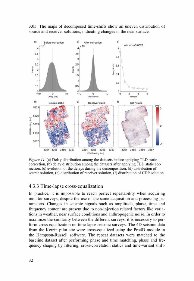
For the second and third repeat surveys, static shifts were derived from the time-lapse differences (Bergmann et al., 2014) instead of re-picking first-breaks for individual survey. By cross-correlating prestack traces between the baseline and repeat surveys within a fixed time window, the time-lapse differences (TLD) were obtained. This data-driven TLD static correction method shows time-efficiency and less time-lapse noise. Figure 11 shows the application of TLD static corrections to the third repeat survey. It is clearly seen that the initial time-lapse bias of about -1 ms among the datasets is re-moved. After 5 iterations the root-mean-square (RMS) decreases from 3.9 to

32

3.05. The maps of decomposed time-shifts show an uneven distribution of source and receiver solutions, indicating changes in the near surface.

Figure 11. (a) Delay distribution among the datasets before applying TLD static correction, (b) delay distribution among the datasets after applying TLD static cor-rection, (c) evolution of the delays during the decomposition, (d) distribution of source solution, (e) distribution of receiver solution, (f) distribution of CDP solution.

4.3.3 Time-lapse cross-equalization In practice, it is impossible to reach perfect repeatability when acquiring monitor surveys, despite the use of the same acquisition and processing pa-rameters. Changes in seismic signals such as amplitude, phase, time and frequency content are present due to non-injection related factors like varia-tions in weather, near surface conditions and anthropogenic noise. In order to maximize the similarity between the different surveys, it is necessary to per-form cross-equalization on time-lapse seismic surveys. The 4D seismic data from the Ketzin pilot site were cross-equalized using the Pro4D module in the Hampson-Russell software. The repeat datasets were matched to the baseline dataset after performing phase and time matching, phase and fre-quency shaping by filtering, cross-correlation statics and time-variant shift-

33

ing, and cross-normalization. A calibration window above the target reser-voir zone was utilized, as ideally, changes in the data, between surveys are not expected above the reservoir. In addition, the near-surface data (around 0-150 ms) were not included since no obvious seismic reflections exist in this interval. After application of time-lapse cross-equalization, changes associated with the movement of fluids in the subsurface can be recognized by subtracting the repeat volume from the baseline volume. The results of the time-lapse 3D surveys will be presented and discussed in Chapter 5.

The match quality can be measured by calculating normalized root-mean-square (NRMS) deviations between the cross-equalized time-lapse volumes (Kragh and Christie, 2002). Larger NRMS values mean lower repeatability. Figure 12 shows the map of the NRMS values between the baseline and third repeat sub-volumes after cross-equalization. Most of the NRMS values range from 0.2 to 0.4 over the survey area, indicating good repeatability (Miller and Helgerud, 2009). Larger NRMS values are present at the edges of the survey area because of lower fold. Larger NRMS values in the vicinity of the injection site are caused by the injected CO2 and lower fold.

Figure 12. NRMS map of the baseline and first post-injection (third repeat) sub-volumes after cross-equalization. Black dot represents the location of the injection well.

34

4.4 CO2 mass estimation CO2 geological storage projects must prove that CO2 injected is contained within the reservoir. Therefore, quantitative assessment of the injected CO2 mass is very important for understanding the risk of leakage. If CO2 leakage is detected, assessment of the mass of CO2 which has leaked is necessary for designing the most optimal remedial solution.

4.4.1 Seismic-well log approach Generally, the seismic-well log approach can be divided into two parts (Fig-ure 13). Firstly, a relationship between CO2 saturations ( ) and time-lapse amplitude changes (∆ ) is derived from pulsed neutron-gamma (PNG) log data measured in wells (Ivanova et al., 2012; Ivandic et al., 2015). Using this CO2 saturation-amplitude change relationship, the CO2 saturation of each CDP over the whole survey area can be estimated. Secondly, the reservoir velocity at a given CO2 saturation is calculated using the linear ve-locity-saturation relationship (equation 4.3). Consequently, the thickness of the CO2 layer (ℎ) can be obtained using equation

ℎ = ∆ ∙ ∙ ∙∆ (4.5)

where ∆ is the time-delay calculated between the baseline and repeat sur-veys over windows above and below the reservoir (Ivandic et al., 2015), is the reservoir velocity fully saturated with brine and ∆ is velocity difference between and .

The total estimated CO2 mass ( ) is calculated using the following equation (Arts et al., 2002) = ∑ ℎ ∙ ∙ ∅ ∙ ∙ ∙ (4.6) where is the total number of CDP bins, represents the CDP index, ∅ is the porosity, is the CO2 density and ∙ determines the CDP bin area.

For the field data, thresholds for time-lapse amplitudes and time shifts need to be set up in order to exclude the impact from non-repeatable noise which is spread throughout the survey area (Ivandic et al., 2015).

35

Figure 13. The workflow of the seismic-well log approach used at the Ketzin site (Ivanova et al., 2012; Ivandic et al., 2015).

4.4.2 Time-shift approach The mass estimation using the seismic-well log approach relies on two as-sumptions. The first is that the CO2 saturation-amplitude change relationship derived from the PNG logging data is representative for the whole survey area. The second is that accurate thresholds for time-lapse amplitudes and time shifts are set up. Additionally, uncertainty exists in this mass estimation method due to uncertainty in the reservoir parameters. At the Ketzin pilot site, the petrophysical model has several limitations, such as the limited number of core samples used to construct the model, the highly heterogene-ous lithology and the difference in frequency range used for laboratory and surface-seismic experiments.

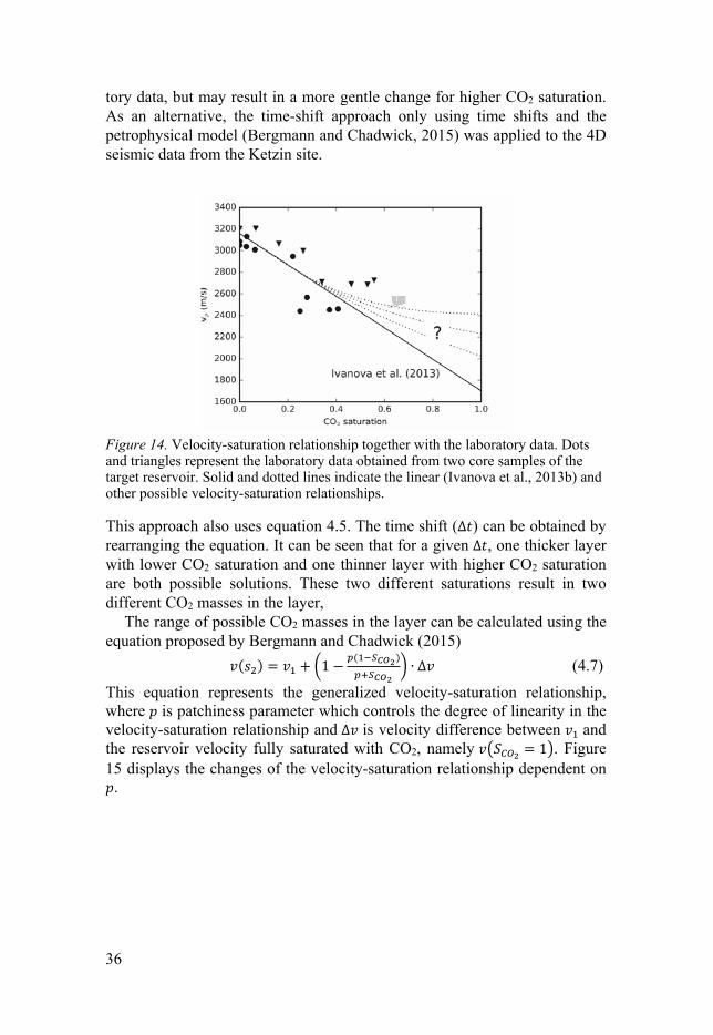
Figure 14 shows the velocity-saturation relationship together with the la-boratory data. Note that the linear relationship fits the laboratory data with CO2 saturation levels of up to 51%, but does not fit well for higher satura-tions. However, CO2 saturations of more than 60 % (up to 100% locally in the Ktzi 201 well) have been retrieved from PNG logging data (Ivanova et al., 2012). Therefore, it raises the question of whether the linear patchy satu-ration model is the most appropriate method for CO2 mass estimation. A Gassmann-type model is another possible approach which fits to the labora-

36

tory data, but may result in a more gentle change for higher CO2 saturation. As an alternative, the time-shift approach only using time shifts and the petrophysical model (Bergmann and Chadwick, 2015) was applied to the 4D seismic data from the Ketzin site.

Figure 14. Velocity-saturation relationship together with the laboratory data. Dots and triangles represent the laboratory data obtained from two core samples of the target reservoir. Solid and dotted lines indicate the linear (Ivanova et al., 2013b) and other possible velocity-saturation relationships.

This approach also uses equation 4.5. The time shift (∆ ) can be obtained by rearranging the equation. It can be seen that for a given ∆ , one thicker layer with lower CO2 saturation and one thinner layer with higher CO2 saturation are both possible solutions. These two different saturations result in two different CO2 masses in the layer,

The range of possible CO2 masses in the layer can be calculated using the equation proposed by Bergmann and Chadwick (2015)

( ) = + 1 − ( ) ∙ ∆ (4.7)

This equation represents the generalized velocity-saturation relationship, where is patchiness parameter which controls the degree of linearity in the velocity-saturation relationship and ∆ is velocity difference between and the reservoir velocity fully saturated with CO2, namely = 1 . Figure 15 displays the changes of the velocity-saturation relationship dependent on

.

37

Figure 15. Set of velocity-saturation relationships derived from equation 4.7 using a variable patchiness parameter (marked graphs) after Bergmann and Chadwick (2015).

Once the generalized velocity-saturation relationship has been calibrated against the pre-existing petrophysical model, the upper and lower bounds of CO2 mass can be determined by time shifts. The upper and lower bounds of the total estimated CO2 mass can be computed using the following two equa-tions

= −( ∙ ) ∙ ∙∅∙ ∙( ∆ )∆ ∙ ∑ ∆ (4.8)

and

= −( ∙ ) ∙ ∑ ∙∅∙ ∙ ∙(∆ ∙( ) )∙ ∙∆ ( )∙∆ ∙ ∙ ∆ (4.9)

where ℎ is the maximum thickness of the CO2 layer equal to the thick-ness of the reservoir. For and , if is less than the patchiness parame-ter for the linear velocity-saturation relationship ( = −( + ∆v)/∆v), the former represents the upper bound and the latter represents the lower bound, and vice versa.

38

5. Seismic characterization of the reservoir at the Ketzin pilot site

5.1 Synthetic time-lapse seismograms Simulation of time-lapse seismic responses is an important method in order to understand and predict changes due to injected CO2 in the reservoir. In order to simulate the migrated seismic responses for the baseline 3D survey, synthetic zero-offset seismograms were generated by convolving the extract-ed 40 Hz zero-phase wavelet with reflection coefficients obtained from the baseline property models (Paper I). In comparison with the other 3D simula-tions which require large computational cost, this simulation can be imple-mented in an efficient way without introducing processing artifacts. Figure 16 shows the synthetic baseline sections compared with the real baseline sections which are close to the CO2 injection well. The seismic characteris-tics such as arrival times, amplitudes and polarities between the synthetic and real data are in good agreement, although the real data exhibit more lat-eral variation. To evaluate the similarity, the cross-correlation coefficients between synthetic and real data ranging from 240 to 580 ms were extracted before and after calibration (Figure 17). The improved cross-correlation co-efficients after calibration are clearly recognizable. The average cross-correlation coefficient before calibration is about 0.6, whereas the average value is up to 0.75 after calibration.

39

Figure 16. Synthetic baseline sections (top panel) compared with the real baseline sections (bottom panel). From left to right: inline 1166 and crossline 1098. The red line shows the sonic log of the injection well. The blue line indicates the K2 horizon.

Figure 17. Maps (left panel) and histograms (right panel) of the cross-correlation coefficient between synthetic and real data before (top panel) and after (bottom panel) calibration. Black dot indicates the location of the injection well.

Similarly, the synthetic migrated seismic responses for the first and second repeat surveys were obtained by using the convolution method. Seismic sec-tions from the synthetic and real data at two repeat times are compared in Figure 18. Increases in reflection amplitudes due to the increased impedance contrast after CO2 injection can be observed at the nearly identical positions in both the synthetic and real data.

40

Figure 18. Synthetic repeat sections (top panel) compared with the real repeat sec-tions (bottom panel) along crossline 1098. From left to right: first repeat and second repeat. The red line represents the sonic log of injection well. The blue line indicates the K2 horizon. The green rectangle denotes the target zone.

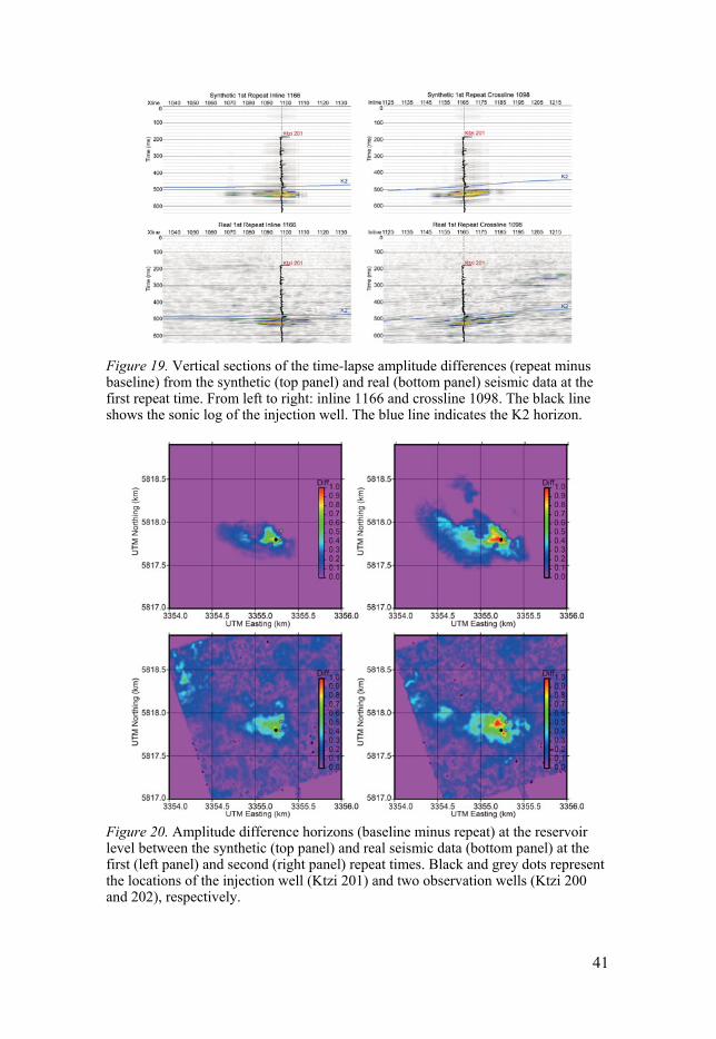
To compare the amplitude anomalies associated with the injected CO2, the vertical sections of the time-lapse amplitude differences from the synthetic and real seismic data at the first repeat time (Figure 19) were acquired by subtracting the repeat volume from the baseline volume. Obvious amplitude anomalies between 515 and 535 ms around the injection well (Ivandic et al., 2012; Ivandic et al., 2013; Ivandic et al., 2015) are comparable between the synthetic and real data. Weak amplitude anomalies observed at deeper levels are related to the push-down effect due to the decrease in reservoir velocity after CO2 injection. In addition, minor anomalies slightly above the reser-voir, but below the K2 reflector, can be seen, despite no CO2 leakage within the overburden. This anomaly may be due to different interference effects of the thin reservoir sandstone before and after CO2 injection, and also non-repeatable noise and processing artifacts in the real data. Figure 20 shows the amplitude difference horizon at the reservoir level between the synthetic and real seismic data at two repeat times. Certain similar features can be found between the synthetic and real maps. The extent of the amplitude anomaly increases from the first repeat time to the second repeat time. More and stronger amplitude anomalies are mapped in the vicinity of the injection well with an increasing amount of injected CO2. The asymmetric distribution of the anomaly is due to the reservoir heterogeneity. However, some differ-ences between the synthetic and real maps are still present. For instance, the size of the synthetic amplitude anomaly which consistently reflects the re-sults of the dynamic flow simulations is smaller than that of the real data, especially at the first repeat time.

41

Figure 19. Vertical sections of the time-lapse amplitude differences (repeat minus baseline) from the synthetic (top panel) and real (bottom panel) seismic data at the first repeat time. From left to right: inline 1166 and crossline 1098. The black line shows the sonic log of the injection well. The blue line indicates the K2 horizon.

Figure 20. Amplitude difference horizons (baseline minus repeat) at the reservoir level between the synthetic (top panel) and real seismic data (bottom panel) at the first (left panel) and second (right panel) repeat times. Black and grey dots represent the locations of the injection well (Ktzi 201) and two observation wells (Ktzi 200 and 202), respectively.

42

5.2 Wavelet phase anomalies related to CO2 injection CSD was applied to the 3D time-lapse datasets with the aim of investigating the changes of the wavelet phase related to the injected CO2 in the reservoir. The vertical sections of the wavelet phase at all frequency bands along an inline close to the injection well were extracted from the baseline, first and second repeat surveys (Figure 21). The range of wavelet phase anomalies in the target area coincides with that of the time-lapse amplitude anomalies in Figure 19. However, a minor amplitude anomaly is seen above the reservoir top, whereas almost no wavelet phase anomaly is detected outside the target area. This implies that the wavelet phase is a stable seismic attribute to de-lineate the top of the CO2 plume. For the baseline survey prior to CO2 injec-tion, the wavelet phase in the sandstone reservoir generally ranges from 60º to 180º, equivalent to yellow, red and magenta colors in the colorbar. -180º and 180º phase are denoted by the same color because a complete cycle is 360 degrees. The wavelet phase horizons are generally continuous despite the lower continuity around the injection well due to the reduced fold. More continuous phase horizons around the injection well are shown after CO2 injection. A wavelet phase of around -120º (blue color) underlying the 180º phase in the reservoir is seen. Utilizing the wavelet phases from 120º to 180º, one can define the location of the reservoir top. The range of the top of the CO2 plume in the reservoir can be further recognized by using the underlying -120º phase. No systematic changes in wavelet phase are detected within the caprock, verifying the integrity of the reservoir. Similar features of wavelet phase anomalies related to CO2 injection are also observed along the other inlines and crosslines close to the injection well (Huang et al., 2016c). A group of monochromatic phase sections were extracted from the first repeat survey in order to investigate the changes of wavelet phase anomalies with frequencies. Results indicate that phase anomalies are mainly concentrated between 30 and 45 Hz (Huang et al., 2016c). The wavelet phases ranging from 120º and 180º with the overlying 60º phase are mainly observed at 30 and 35 Hz, whereas most of the underlying -120º phase is seen at 40 and 45 Hz.

43

Figure 21. Vertical sections of the wavelet phase at all frequency bands along inline 1166 at the (a) baseline, (b) first repeat and (c) second repeat times. The red line represents the location of injection well. The blue lines indicate the approximate locations of the reservoir top and base. The black rectangle denotes the target zone.

44

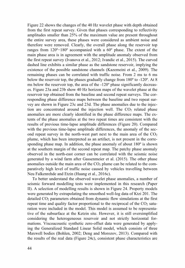
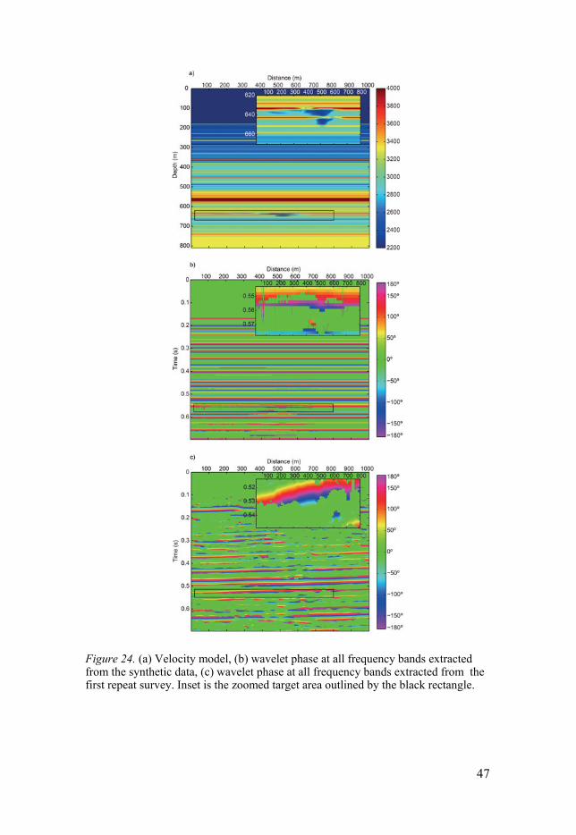
Figure 22 shows the changes of the 40 Hz wavelet phase with depth obtained from the first repeat survey. Given that phases corresponding to reflectivity amplitudes smaller than 25% of the maximum value are present throughout the entire survey area, these phases were considered as ambient noise and therefore were removed. Clearly, the overall phase along the reservoir top ranges from 120º−180º accompanied with a 60º phase. The extent of the main phase area is in agreement with the amplitude anomaly observed from the first repeat survey (Ivanova et al., 2012; Ivandic et al., 2015). The curved dashed line exhibits a similar phase as the sandstone reservoir, implying the existence of the possible sandstone channels (Kazemeini et al., 2009). The remaining phases can be correlated with traffic noise. From 2 ms to 6 ms below the reservoir top, the phases gradually change from 180º to -120º. At 8 ms below the reservoir top, the area of the -120º phase significantly decreas-es. Figure 23a and 23b show 40 Hz horizon maps of the wavelet phase at the reservoir top obtained from the baseline and second repeat surveys. The cor-responding phase difference maps between the baseline and two repeat sur-vey are shown in Figure 23c and 23d. The phase anomalies due to the injec-tion are concentrated around the injection well. The CO2 related phase anomalies are more clearly identified in the phase difference maps. The ex-tents of the phase anomalies at the two repeat times are consistent with the results of previous time-lapse amplitude differences (Figure 20). Compared with the previous time-lapse amplitude differences, the anomaly of the sec-ond repeat survey in the north-west part next to the main area of the CO2 plume, which has been interpreted as an artifact, is not present in the corre-sponding phase map. In addition, the phase anomaly of about 180º is shown at the southern margin of the second repeat map. The patchy phase anomaly observed in the north-east corner can be correlated with the seismic noise generated by a wind farm after Gassenmeier et al. (2015). The other phase anomalies outside the main area of the CO2 plume can be related to the com-paratively high level of traffic noise caused by vehicles travelling between Neu Falkenrehde and Etzin (Huang et al., 2016c).

To better understand the observed wavelet phase anomalies, a number of seismic forward modelling tests were implemented in this research (Paper II). A selection of modelling results is shown in Figure 24. Property models were generated by extrapolating the smoothed well-log data of Ktzi 201. The detailed CO2 parameters obtained from dynamic flow simulations at the first repeat time and quality factor proportional to the reciprocal of the CO2 satu-ration were included in the model. This model is assumed to be representa-tive of the subsurface at the Ketzin site. However, it is still oversimplified considering the heterogeneous reservoir and not strictly horizontal for-mations. Viscoacoustic synthetic zero-offset data were generated by apply-ing the Generalized Standard Linear Solid model, which consists of three Maxwell bodies (Bohlen, 2002; Deng and Morozov, 2013). Compared with the results of the real data (Figure 24c), consistent phase characteristics are

45

observed in the synthetic data (Figure 24b). The lateral range of the -120º phase almost coincides with the distribution of the CO2 plume in the reser-voir. Phases of 120º−180º accompanied with a 60º phase are also observed. In addition, analysis of the simulation results reveals that the phase anoma-lies related to CO2 injection at the Ketzin site can be mainly attributed to interference rather than an offset-dependent effect. This was proved by the identical phase results obtained from the real data within only near-offsets and all offsets.

Figure 22. Changes of the 40 Hz wavelet phase with depth obtained from the first repeat survey. From top to bottom: at the top of the reservoir, 2 ms, 4 ms, 6 ms, and 8 ms below the top of the reservoir. The white solid line represents the outline of the imaged CO2 plume for the first repeat survey. The curved dashed represents possible sandstone channels. Black and grey dots represent the locations of the injection well (Ktzi 201) and three observation wells (Ktzi 200, 202 and 203), respectively.

46

Figure 23. 40-Hz horizon maps of the wavelet phase at the top of the reservoir for (a) baseline, (b) second repeat. (c) and (d) are the corresponding wavelet phase dif-ference, respectively. The white solid lines represent the outlines of the imaged CO2 plume for the first and second repeat surveys. The curved dashed lines represents possible sandstone channels. Black and grey dots represent the locations of the injec-tion well (Ktzi 201) and three observation wells (Ktzi 200, 202 and 203), respective-ly.

47

Figure 24. (a) Velocity model, (b) wavelet phase at all frequency bands extracted from the synthetic data, (c) wavelet phase at all frequency bands extracted from the first repeat survey. Inset is the zoomed target area outlined by the black rectangle.

48

5.3 Reservoir thickness A number of spectral decomposition methods like CWT and WVD have been performed to estimate the thickness of the injected CO2 using the tun-ing frequency-temporal thickness relationship at the Sleipner project site and the Snøhvit gas field (Chadwick et al., 2010; Ravazzoli and Gómez, 2014). At the Ketzin site, Kazemeini et al. (2009) previously used the CWT method to qualitatively analyze the reservoir details. Given several limitations at the Ketzin site (such as thin sandstone layers, limited resolution of band-limited conventional seismic data, inevitable noise in a semi-urban site and presence of the thin high-velocity anhydrite layer), the CSD method with higher time-frequency resolution and less sensitivity to noise is the optimal option for quantitatively evaluating the thickness of the reservoir.

We extracted a batch of monochromatic reflectivity amplitude sections which were aimed at providing a first visual estimate of reservoir thicknesses for tuning frequency extraction (Paper III). A comparison of the convention-al baseline sections and the corresponding reflectivity amplitude sections are shown in Figure 25. The reflectivity amplitude sections detail the structure with higher temporal resolution. The discontinuity imaged at east and south of the injection well coincides with the reservoir heterogeneity and can be used to interpret the preferred orientation of CO2 propagation (Ivandic et al., 2015). The source wavelet extracted from well logging and seismic data within 200-800 ms in the vicinity of the injection site was then used to bal-ance the amplitude spectrum of the reservoir.

Figure 26 shows the tuning frequencies of the sandstone units determined from the balanced spectrum of the baseline survey. The range of tuning fre-quency is 50-80 Hz, equivalent to a two-way temporal thickness of 6.3-10 ms. The thickness of the reservoir sandstone can be calculated using the average velocity of the reservoir sandstone fully saturated with brine at the Ketzin site (3135 m/s) (Ivanova et al., 2012). The calculated thickness rang-es from 9.7 m to 17.4 m, which is in good agreement with the sandstone thickness of 9–20 m measured from logging data (Förster et al., 2010).

49

Figure 25. Comparison of the conventional baseline sections (top panel) and the corresponding reflectivity amplitude sections (bottom panel). From left to right: inline 1166 and crossline 1098. The black vertical line represents the location of injection well. The black horizontal lines indicate the approximate locations of the K2 horizon and reservoir.

Figure 26. Tuning frequencies of sandstone units extracted from the baseline survey. White and grey dots represent the locations of the injection well (Ktzi 201) and three observation wells (Ktzi 200, 202 and 203), respectively.

50

Figure 27 shows the tuning frequencies of gaseous CO2 determined from the balanced amplitude spectra of the time-lapse amplitude differences at two repeat times. The extent of the gaseous CO2 was defined by using an amplitude threshold of 0.25 at the reservoir level to exclude the remaining non-repeatable noise (Ivandic et al., 2015). Much higher tuning frequencies, which are present at north, south and east of the injection site, can be as-sumed as the low-permeability CO2 migration pathways to explain the pre-dominant WNW trend of the gaseous CO2 movement. The calculated tem-poral thicknesses of the gaseous CO2 plume at four wells (Ktzi 200, 201, 202 and 203) are presented in Table 5.1. There is no determined tuning frequen-cy for the Ktzi 200 well at the first repeat time. From the first repeat time to the second repeat time, the increased temporal thicknesses of the gaseous CO2 are found in all four wells, while a greater increase is observed in the Ktzi 203 well. This shows that more CO2 moves towards the north of the injection well, namely the up-dip direction. The calculated temporal thick-nesses at the second repeat time reflect the variation of sandstone thickness in four wells. The velocity of the reservoir saturated with 50% CO2 was used to estimate the thicknesses of the gaseous CO2 in the Ktzi 201 well at two repeat times. The estimated values (21.7 and 23.3 m) are a bit higher than the actual net thickness of the reservoir sandstone in the Ktzi 201 well (19 m) but reasonable since CO2 was also observed in a thinner silt- and sandstone layer beneath the main-reservoir sandstone in the injection well (Ivanova et al., 2012; Baumann et al., 2014).

Figure 27. Tuning frequencies of gaseous CO2 extracted from the first (left panel) and second (right panel) repeat surveys. White and grey dots represent the locations of the injection well (Ktzi 201) and three observation wells (Ktzi 200, 202 and 203), respectively.

51

Table 5.1. Thickness of the reservoir sandstone compared with calculated temporal thickness of the gaseous CO2 plume.

Well Reservoir sandstone (m)

Gaseous CO2 plume (ms)1st repeat 2nd repeat

Ktzi 200 16 - 14.2Ktzi 201 19 18.3 19.7Ktzi 202 9 8.3 8.5Ktzi 203 18 7.5 17.1

5.4 Discrimination between CO2 saturation and pressure changes The amplitude anomalies caused by the pressure and fluid saturation changes can be discriminated by using time-lapse amplitude variation with offset (AVO) (Landrø, 2001; Landrø et al., 2003; Grude et al., 2013). However, this approach has not achieved success at the Ketzin site (Ivanova et al., 2013a) because of limited signal-to-noise ratio, relatively short offsets and the presence of a thin but high-velocity anhydrite layer.

After CO2 injection, pore pressure increases and consequently effective stress in the formation decreases. This gives a rise to decrease in seismic velocity. Therefore, similar changes in seismic amplitude as those caused by CO2 saturation may occur in the formation. Given the assumption that the change of the pore pressure spreads in the entire reservoir height and the gaseous CO2 saturation is mainly present within the upper reservoir interval (White et al., 2015), it is possible to utilize distinct tuning to discriminate the saturation and pressure effects. Considering that there is no available S-wave data in the 4D seismic from the Ketzin site, discrimination between CO2 saturation and pressure changes using tuning frequency of P-wave data is feasible.

Based on the sandstone thickness determined from the baseline survey (Figure 26), the tuning frequencies of the corresponding sandstone fully saturated with CO2 were estimated from simulation results (Section 4.2.3). These estimates were considered as the theoretical lower limits of the tuning frequencies after CO2 injection. If the tuning frequency from the repeat sur-veys are larger than the threshold, it indicates that the saturation effect over-whelms the pressure effect, and vice-versa (Huang et al., 2016b). In this way, the pressure and fluid saturation changes can be separated from each other. Anomaly maps of CO2 saturation and apparent pressure at two repeat times are shown in Figure 28. In comparison with the second repeat survey, more pressure related anomalies are mapped from the first repeat survey, which is in agreement with the significant reduction in downhole pressure measured at the second repeat time (Martens et al., 2014). It is clearly seen

52

that the majority of the amplitude anomaly is caused by CO2 saturation at the Ketzin site, implying the presence of the connected sandstone channels mainly in the west and north of the injection site.

Quantitative assessment of the CO2 mass was implemented based on the determined tuning frequency instead of the time delays which were used in the previous studies. Compared with the time delays estimated from the con-ventional seismic reflections, the tuning frequency is not influenced by the phase distortion during the data processing and can determine the thickness of thin layers below the conventional seismic resolution. In addition, pres-sure related anomalies can be excluded when calculating CO2 mass. Howev-er, a discrepancy between the injected and calculated CO2 mass still exists due to several uncertainties: ongoing CO2 dissolution, error of determined tuning frequency, reservoir heterogeneity, etc (Paper III).

Figure 28. Anomaly maps of CO2 saturation (left panel) and apparent pressure (right panel) at two repeat times. From top to bottom: the first and second repeat times. White and grey dots represent the locations of the injection well (Ktzi 201) and three observation wells (Ktzi 200, 202 and 203), respectively.

53

5.5 Time-lapse analysis of the first post-injection survey Vertical sections of the time-lapse amplitude difference close to the injection well for three repeat surveys are shown in Figure 29. The accumulation of CO2 within the reservoir is imaged by the notable amplitude changes be-tween 515 ms and 535 ms two-way traveltime (TWT) (Ivanova et al., 2012; Ivandic et al., 2015). From the first repeat time to the second repeat time, further growth and migration of the amplitude anomaly in the reservoir was observed. The first post-injection survey shows a decrease in intensity and in the extent of the amplitude anomaly with a weaker push-down effect at deeper levels compared to the second repeat survey. In agreement with the previous results, a tendency of movement in the up-dip direction within the reservoir is revealed. No systematic anomalies above the K2 are observed.

Figure 29. Vertical sections of time-lapse amplitude difference (repeat minus base-line) for three repeat surveys along inline 1166 (left panel) and crossline 1100 (right panel). From top to bottom: first repeat, second repeat and first post-injection (third repeat) results. The black line shows the location of the injection well. The red line indicates the K2 horizon.

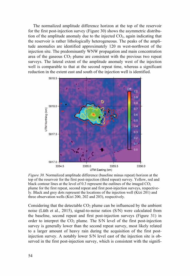
54

The normalized amplitude difference horizon at the top of the reservoir for the first post-injection survey (Figure 30) shows the asymmetric distribu-tion of the amplitude anomaly due to the injected CO2, again indicating that the reservoir is rather lithologically heterogeneous. The peaks of the ampli-tude anomalies are identified approximately 120 m west-northwest of the injection site. The predominantly WNW propagation and main concentration area of the gaseous CO2 plume are consistent with the previous two repeat surveys. The lateral extent of the amplitude anomaly west of the injection well is comparable to that at the second repeat time, whereas a significant reduction in the extent east and south of the injection well is identified.

Figure 30. Normalized amplitude difference (baseline minus repeat) horizon at the top of the reservoir for the first post-injection (third repeat) survey. Yellow, red and black contour lines at the level of 0.3 represent the outlines of the imaged CO2 plume for the first repeat, second repeat and first post-injection surveys, respective-ly. Black and grey dots represent the locations of the injection well (Ktzi 201) and three observation wells (Ktzi 200, 202 and 203), respectively.

Considering that the detectable CO2 plume can be influenced by the ambient noise (Lüth et al., 2015), signal-to-noise ratios (S/N) were calculated from the baseline, second repeat and first post-injection surveys (Figure 31) in order to interpret the CO2 plume. The S/N level of the first post-injection survey is generally lower than the second repeat survey, most likely related to a larger amount of heavy rain during the acquisition of the first post-injection survey. A notably lower S/N level east of the injection site is ob-served in the first post-injection survey, which is consistent with the signifi-

55

cant reduction of the amplitude anomaly in the corresponding area. This indicates that the lower S/N level may be one of the factors related to the decrease in amplitude anomaly in this area.

Figure 31. Maps of ratio of S/N. Top: 2012/2005, bottom: 2015/2005. Red dot rep-resents the location of the injection well.

Seismic simulation based on the detailed 3D seismic property models for the first post-injection survey was performed in order to better understand the changes in amplitude anomaly (Paper IV). The amplitude difference horizon at the reservoir level for the synthetic first post-injection survey is shown in Figure 32. Almost the same extents of the synthetic amplitude anomalies at the second repeat and first post-injection times are mapped, consistent with the similar features observed west of the injection site in field data (Figure 30). According to the dynamic flow simulations, up to 27 % of the CO2 was dissolved at the relevant times and is undetectable for 4D seismic measure-ments. Considering the wide-ranging CO2-brine contact in the heterogeneous reservoir and comparatively low injection rates, the relatively high CO2 dis-solution rate is reasonable. The dynamic flow simulations also reveal that the areal extent of thin layers has increased by 30 % since the second repeat time. This indicates that a dynamic balance between newly injected CO2 (6 kt more injected after the second repeat time) and the CO2 undergoing disso-lution/diffusion was reached by the time of the first post-injection survey.

56

Figure 32. Amplitude difference horizon at the reservoir level for the synthetic first post-injection (third repeat) survey. Red and black contour lines at the level of 0.1 represent the outlines of the imaged CO2 plume for the second repeat and first post-injection surveys. Black and grey dots represent the locations of the injection well (Ktzi 201) and three observation wells (Ktzi 200, 202 and 203), respectively.

5.6 Quantitative assessment of the CO2 mass Time-delays by calculating the time difference between the baseline and first post-injection surveys over windows above and below the reservoir are shown in Figure 33. Note that few obvious time-delays exist near the injec-tion site, whereas amplitude anomalies are mapped in the amplitude differ-ence horizon from the first post-injection survey (Figure 30). This could be related to the impact of the brine injection in the CO2 storage horizon from October 2015 to January 2016 (Möller et al., 2016).

57

Figure 33. Time-delays by calculating the time difference between the baseline and first post-injection (third repeat) surveys. Black dot represents the location of the injection well. The black rectangle denotes the area used for CO2 mass quantifica-tions.

The detectable masses of the gaseous CO2 plume at three repeat times were firstly estimated by using the seismic-well log approach. The same parame-ters except for the density of CO2 derived from a different pres-sure/temperature were used for all the surveys. In the previous studies at the Ketzin site (Ivanova et al., 2012; Ivandic et al., 2015), CO2 saturations re-trieved from the PNG logs at the relevant times were used (Ivanova et al., 2012; Ivandic et al., 2015). In this study, the same saturation model which was previously used for the first repeat survey was applied to all three repeat surveys with the aim of providing a consistent methodology for CO2 mass estimation (Table 5.2). These saturations are close to the values obtained from the PNG logging data, but do not correspond exactly to them. The total estimated CO2 mass for the first post-injection survey is 10.8 kt, which is 16 % of the actual injected amount of CO2. This discrepancy (84 %) is much larger than for the first and second repeat surveys (10-15 %). The difference between the estimated CO2 mass in this study and in the previous study (Ivanova et al., 2012) can be ascribed to interpolation from geographic coor-dinates. Using saturations retrieved from the PNG logging data which were acquired at the time of the first post-injection survey, the total estimated CO2 mass is 13 kt, still significantly smaller than the actual injected amount of CO2. However, this estimate is not unreasonable since a dramatic reduction in mass with time is also observed in the simulations. In addition to limited understanding of the heterogeneous reservoir, several factors, such as CO2 dissolution and diffusion, limited seismic resolution and ambient noise, lead to the significant decrease in mass estimate. The brine injection may also

58

have influence on the mass due to the absent time-delays around the injec-tion well. Figure 34 shows that the different choices of uncertain reservoir parameters result in mass variation of the first post-injection survey. The estimated mass is most susceptible to the choices of time-delay cutoff and reservoir velocity.

Table 5.2. Respective parameter choices for the three repeat surveys.

Conversion of normal-ized 4D amplitude (Δ ) to CO2 saturation ( )

Density of CO2 (kg/m3)

Poro-sity (%)

Normalized 4D ampli-tude threshold

Time shift Threshold (ms)

Calculated mass (kt)

Repeat 1 (Ivanova et al., 2012)

= 33%, Δ 0.442%, 0.4 Δ 0.648%, Δ > 0.6266.62 20 0.3 1.5 23.83

Repeat 2 (Ivandic et al., 2015)

= 50% 215 20 0.3 1.5 52.51

Repeat 1 (this study)

= 33%, Δ 0.442%, 0.4 Δ 0.648%, Δ > 0.6266.62 20 0.3 1.5 26.84

Repeat 2 (this study)

= 33%, Δ 0.442%, 0.4 Δ 0.648%, Δ > 0.6215 20 0.3 1.5 55.66

Repeat 3 (this study) = 33%, Δ 0.442%, 0.4 Δ 0.648%, Δ > 0.6

184.2 20 0.3 1.5 10.80

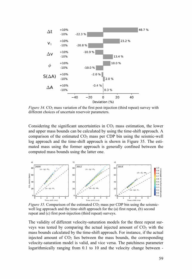
59

Figure 34. CO2 mass variation of the first post-injection (third repeat) survey with different choices of uncertain reservoir parameters.

Considering the significant uncertainties in CO2 mass estimation, the lower and upper mass bounds can be calculated by using the time-shift approach. A comparison of the estimated CO2 mass per CDP bin using the seismic-well log approach and the time-shift approach is shown in Figure 35. The esti-mated mass using the former approach is generally confined between the computed mass bounds using the latter one.

Figure 35. Comparison of the estimated CO2 mass per CDP bin using the seismic-well log approach and the time-shift approach for the (a) first repeat, (b) second repeat and (c) first post-injection (third repeat) surveys.

The validity of different velocity-saturation models for the three repeat sur-veys was tested by comparing the actual injected amount of CO2 with the mass bounds calculated by the time-shift approach. For instance, if the actual injected amount of CO2 lies between the mass bounds, the corresponding velocity-saturation model is valid, and vice versa. The patchiness parameter logarithmically ranging from 0.1 to 10 and the velocity change between -

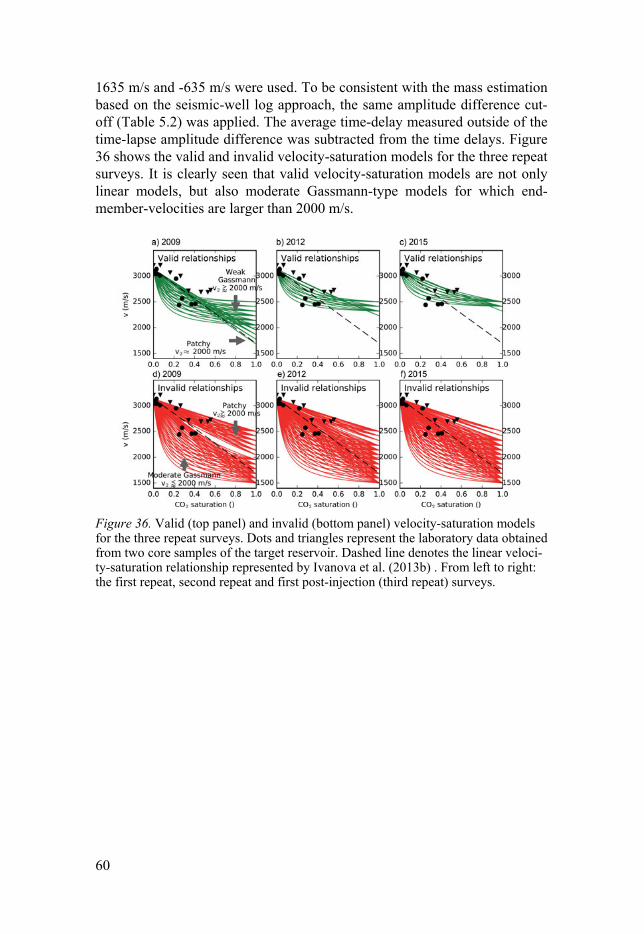
60

1635 m/s and -635 m/s were used. To be consistent with the mass estimation based on the seismic-well log approach, the same amplitude difference cut-off (Table 5.2) was applied. The average time-delay measured outside of the time-lapse amplitude difference was subtracted from the time delays. Figure 36 shows the valid and invalid velocity-saturation models for the three repeat surveys. It is clearly seen that valid velocity-saturation models are not only linear models, but also moderate Gassmann-type models for which end-member-velocities are larger than 2000 m/s.

Figure 36. Valid (top panel) and invalid (bottom panel) velocity-saturation models for the three repeat surveys. Dots and triangles represent the laboratory data obtained from two core samples of the target reservoir. Dashed line denotes the linear veloci-ty-saturation relationship represented by Ivanova et al. (2013b) . From left to right: the first repeat, second repeat and first post-injection (third repeat) surveys.

61

6. Conclusions and outlook

6.1 Conclusions This thesis provides a number of studies with respect to utilizing 3D time-lapse analysis of seismic reflection data to characterize the reservoir at the Ketzin pilot site. The following overall conclusions are drawn with regards to the four objectives addressed in Chapter 1. 1. To efficiently integrate the existing borehole data and the 3D seismic

data to build detailed 3D seismic property models for seismic simulation at the Ketzin pilot site:

• Detailed 3D property models were built by integrating borehole data and 3D reflection seismic data in an efficient way. Changes in P-wave velocity and density at repeat times were calculated using CO2 satura-tions and densities derived from history-matched dynamic flow simu-lations.

• Pseudo-boreholes between and beyond well control were constructed. Comparison of the pseudo- and original logs for the Ktzi 200 well shows a good agreement.

• Time-lapse synthetic zero-offset seismograms were achieved using the convolution method with the aim of efficient implementation without introducing processing artifacts. Good similarity between real and synthetic data at times of the baseline and repeat surveys indicates that the constructed 3D property models are, in general, reliable represen-tations of the subsurface conditions in the vicinity of the site. Some differences between the synthetic and real time-lapse results still exist, mainly due to non-representative parameterization and poor quality of the seismic data in the near-wellbore area of less coverage.

2. To investigate the feasibility of utilizing wavelet phase changes related to the CO2 plume to reduce the uncertainty in monitoring CO2 distribu-tion:

• Continuous horizons of wavelet phase were obtained from the 3D time-lapse seismic data after application of complex spectral decom-position, despite this procedure being performed trace by trace.

• Changes in wavelet phase related to the CO2 plume were observed. The lateral range of the CO2 plume in the reservoir was identified us-ing the vertical sections of wavelet phase, consistent with the results

62

of the previous time-lapse amplitude differences. Additionally, the top of the reservoir was better delineated.

• A series of seismic modelling tests were performed and show con-sistent phase results as observed from the field data. The phase anomaly related to CO2 at the Ketzin site was most likely due to the interference effect in the thin sandstone reservoir.

• Distinguished phase anomalies associated with noise and the CO2 plume were mapped using the phase difference horizon at the reser-voir level. Combining wavelet phase characteristics with the ampli-tude attribute can decrease uncertainty in detecting the CO2 plume in the reservoir.

3. To determine tuning frequency to quantitatively assess the thickness and mass of the gaseous CO2 and to attempt the discrimination between pres-sure effect and CO2 saturation:

• Tuning frequencies were determined by applying complex spectral decomposition to the 3D time-lapse seismic data. The calculated thicknesses reflect the thickness variation of the reservoir sandstone and gaseous CO2.

• Compared with the conventional 3D data, reflectivity amplitude sec-tions show more layer details with higher temporal resolution. Ab-normally high tuning frequencies to the north, south and east of the in-jection site were observed in the tuning frequency maps at two repeat times, supporting the predominant WNW trend of the gaseous CO2 migration.

• The amplitude anomalies caused by the pressure and CO2 saturation changes were discriminated, showing that the amplitude anomaly at the Ketzin site is mainly due to CO2 saturation. Quantitative assess-ment of the CO2 mass based on the tuning frequency related to CO2 saturation was performed but contains some uncertainties.

4. To evaluate the recent development of the CO2 plume in the post-closure phase and to estimate CO2 mass using two different models (patchy and non-patchy saturation models):

• The first post-injection (third repeat) survey with approximately 5700 source points was acquired and processed. Time-lapse analysis of the first post-injection survey indicates that the intensity and size of the amplitude anomaly have decreased since the second repeat survey. In agreement with the previous time-lapse results, a preferred WNW ten-dency of CO2 movement in the up-dip direction is observed. No evi-dence of systematic anomalies above the caprock is detected.

• Seismic simulation reveals that a dynamic balance between the newly injected CO2 after the second repeat time and the CO2 undergoing dis-solution/diffusion was reached by the time of the first post-injection survey.

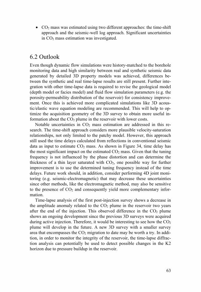
63

• CO2 mass was estimated using two different approaches: the time-shift approach and the seismic-well log approach. Significant uncertainties in CO2 mass estimation was investigated.

6.2 Outlook Even though dynamic flow simulations were history-matched to the borehole monitoring data and high similarity between real and synthetic seismic data generated by detailed 3D property models was achieved, differences be-tween the synthetic and real time-lapse results are still present. Further inte-gration with other time-lapse data is required to revise the geological model (depth model or facies model) and fluid flow simulation parameters (e.g. the porosity-permeability distribution of the reservoir) for consistency improve-ment. Once this is achieved more complicated simulations like 3D acous-tic/elastic wave equation modeling are recommended. This will help to op-timize the acquisition geometry of the 3D survey to obtain more useful in-formation about the CO2 plume in the reservoir with lower costs.

Notable uncertainties in CO2 mass estimation are addressed in this re-search. The time-shift approach considers more plausible velocity-saturation relationships, not only limited to the patchy model. However, this approach still used the time delays calculated from reflections in conventional seismic data as input to estimate CO2 mass. As shown in Figure 34, time delay has the most significant impact on the estimated CO2 mass. Given that the tuning frequency is not influenced by the phase distortion and can determine the thickness of a thin layer saturated with CO2, one possible way for further improvement is to use the determined tuning frequency instead of the time delays. Future work should, in addition, consider performing 4D joint moni-toring (e.g. seismic-electromagnetic) that may decrease these uncertainties since other methods, like the electromagnetic method, may also be sensitive to the presence of CO2 and consequently yield more complementary infor-mation.

Time-lapse analysis of the first post-injection survey shows a decrease in the amplitude anomaly related to the CO2 plume in the reservoir two years after the end of the injection. This observed difference in the CO2 plume shows an ongoing development since the previous 3D surveys were acquired during active injection. Therefore, it would be interesting to see how the CO2 plume will develop in the future. A new 3D survey with a smaller survey area that encompasses the CO2 migration to date may be worth a try. In addi-tion, in order to monitor the integrity of the reservoir, the time-lapse diffrac-tion analysis can potentially be used to detect possible changes in the K2 horizon due to pressure buildup in the reservoir.

64

7. Summary in Swedish

Denna avhandling omfattar ett flertal studier som karakteriserar koldioxidreservoaren vid Ketzin’s pilotanläggning och hur den förändras med tiden genom analys av reflektionsseismiskt 3D data. Fyra övergripande objektiv definieras här nedan och utifrån dessa har ett flertal slutsatser dragits.

1. Integrera befintliga borrhålsdata med 3D seismiskt data på ett effektivt

sätt för att konstruera en detaljerad 3D modell av seismiska egenskaper för seismiska simuleringar vid Ketzin’s pilotanläggning.

• En detaljerad 3D modell av seismiska egenskaper har konstruerats genom att effektivt integrera borrhålsdata med reflektionsseismiskt 3D data. Förändringar i P-vågshastighet och densitet beräknades vid tidpunkterna för de återkommande seismiska undersökningar utifrån koldioxidmättnad och densitet som uppskattats genom dynamiska flödessimuleringar.

• Utifrån denna modell har syntetiska borrhål skapats mellan och bortanför de verkliga borrhålen. Vid jämförelse visar syntetiska loggar från de syntetiska borrhålen god överensstämmelse med verkliga loggar från borrhålet Ktzi 200.

• Syntetiska seismogram med gemensam källa och mottagare (zero-offset) som visar förändringar i tiden har konstruerats på ett effektivt sätt utan att introducera databehandlingsartefakter genom att använda faltning. Syntetiskt och verkligt data från tidpunkterna för den ursprungliga och de efterföljande upprepade mätningarna stämmer väl överens. Detta tyder på att den konstruerade 3D modellen över seismiska egenskaper generellt sett representerar förhållandena under jordytan väl i området runt anläggningen. Vissa skillnader finns dock på grund av en icke representativ parameterisering samt en lägre seismisk datakvalité precis vid borrhålen eftersom färre instrument kunde placeras där.

2. Undersöka om det är lämpligt att använda de fasförändringar som orsakas av koldioxidutbredningen för att reducera osäkerheterna vid övervakning av förändringar i koldioxidens utbredning.

65

• Komplex spektral upplösning (decomposition) har använts för att, utifrån 3D seismiska data från de upprepade mätningarna, skapa kontinuerliga horisonter av vågformernas fas. Denna procedur är dock krävande då den måste utföras separat för varje seismogram.

• Förändringar i vågformernas fas observeras i direkt relation till koldioxidutbredninen. Den horisontella utbredningen av injicerat CO2 i reservoaren identifierades i vertikala sektioner över vågformernas fas och överensstämmer väl med de amplitudförändringar som tidigare observerats med tiden. Dessutom har reservoarens takgräns kunnat definieras tydligare.

• En serie seismiska modelleringstester visar på att de observerade faserna stämmer väl överens med resultaten från insamlade data. Fasanomalin som är kopplad till det CO2 som injicerats vid anläggningen i Ketzin orsakas troligtvis av interferenseffekter i den tunna sandstensreservoaren.

• Utifrån horisonter av fasskillnader på djup motsvarande reservoaren, har fasanomalier som associeras med brus respektive injicerat CO2 identifierats och kartlagts. Osäkerheter i att identifiera injicerat CO2 kan minimeras genom att kombinera vågformernas fas- och amplitudegenskaper.

3. Göra en kvantitativ uppskattning av mängden injicerat CO2 och dess massa genom beräkning av frekvensen där mest konstruktiv interferens sker (tuning frequency), samt särskilja mellan effekter orsakade av förändringar i tryck och koldioxidmättnad.

• Tuningfrekvenser har bestämts med hjälp av komplex spektral upplösning av seismiska 3D data från upprepade mätningar. Den beräknade tjockleken representerar variationer i både reservoarsandstenens tjocklek och mängden koldioxid i gasfas.

• Sektioner som visar reflektivitetsamplituder har högre vertikal upplösning och visar mer detaljer jämfört med konventionella 3D data. Onormalt höga tuningfrekvenser i områdena till norr, söder och öster om anläggningen kan ses i horisontella tvärsnitt över tuningfrekvensen vid två upprepade mätningar. Detta stämmer överens med den observerade utbredningen av den gasformiga koldioxiden mot västnordväst.

• Amplitudanomalier som orsakas av förändringar i tryck respektive koldioxidmättnad har urskilts och visar att amplitudanomalin vid anläggningen i Ketzin huvudsakligen kan härledas till mättnaden av CO2. Baserat på tuningfrekvensen, som påverkas av koldioxidmättnad, har en kvantitativ bedömning av den injicerade koldioxidens massa gjorts, dock med viss osäkerhet.

4. Bestämma koldioxidens utbredning efter avslutad injicering och uppskatta den injicerade koldioxidens massa med hjälp av två olika modeller; de så kallade "patchy" och "non-patchy" mättnadsmodellerna.

66

• Den första seismiska mätningen efter avslutad injektion genomfördes med ca 5700 källpunkter och den efterföljande processeringen är slutförd. Analys av förändringar med tiden efter avslutad injektion tyder på en minskad intensitet och horisontell utbredning jämfört med den andra upprepade mätningen under pågående injektion. Precis som med föregående mätningar verkar koldioxiden ha en benägenhet att migrera mot västnordväst. Inga tecken på anomalier kan observeras ovanför caprocken.

• Seismiska simuleringar visar att det, vid tidpunkten för den första mätningen efter avslutad injektion, uppstått en dynamisk balans mellan koldioxiden som injicerades efter den andra upprepade mätningen och koldioxiden som håller på att lösas upp eller spridas.

• Den injicerade koldioxidens massa har uppskattats både med tidsförskjutningsmetoden och med log-seismik metoden. Även osäkerheter i dessa uppskattningar har undersökts.

67

Acknowledgements

Performing PhD research is a privileged journey not only because of the invaluable knowledge and skills one gains, but also because of a wonderful people one meets on the path to progress. This thesis would not have been possible without the encouragement, support and help from many friendly individuals during the four years.

Above all I would like to thank my main supervisor Christopher Juhlin for guiding and supporting me in getting to this point. You are a great super-visor on both the academic and personal level. I appreciate that you intro-duced me to academic life and always had time to discuss my research. You always gave swift feedback about my questions. Whenever I sent a manu-script to you, within one or two days I would get the revised one with signif-icant improvement of the English and structure. Your time management skill and enthusiasm for research inspired me. You gave me the freedom to pur-sue my interested studies. I feel very fortunate to be your PhD student. I would also like to thank my co-supervisors Alireza Malehmir and Ari Tryggvason for your time, ideas and advice. I learned a lot from the lectures you presented and the chats we had. I am very thankful to Martin Landrø for providing me the opportunity to visit Norwegian University of Science and Technology (NTNU). Your valuable comments and suggestions enhanced my understanding of seismic reservoir characterization. Thank you Thomas Kalscheuer for your discussion about electromagnetic methods.

Special thanks to Hans Palm for your excellent organizational abilities and fieldwork knowledge. I still clearly remember that on the first day when I arrived at Ketzin, you taught me the working principle of the field equip-ment and how to plant geophones. You are my field supervisor. I would also like to thank you for inviting us to celebrate the Swedish mid-summer and Christmas festivals with you. I will keep all the wonderful gifts you gave for missing you forever.

Thank you Monika Ivandic and Fengjiao Zhang, for providing great help throughout my PhD journey. Without your help with seismic processing, I cannot imagine how tough it would be when I commenced my project. I would like to thank Daniel Sopher for your kind collaboration and important discussions. I am grateful to the other co-authors, Stefan Lüth, Thomas Kempka, Ben Norden, Alexandra Ivanova, Jan Henninges from GFZ Ger-man Research Centre, Li Han from CNOOC Research Institute and Wubing Deng from University of Saskatchewan for collaborating with me and giving

68

useful feedback on my work. I am also thankful to Peter Bergmann for shar-ing your codes and taking time to discuss with me. Thank you Dibakar Ghosal and Jochen Kamm for all the useful discussions. Thanks to Shibo Xu, Qi Hao and Sissel Grude for helping me during my stay at NTNU. I would like to thank all the editors and reviewers for their constructive com-ments that helped to improve my papers.

I want to especially thank Peter Hedin, Daniel Sopher, Monika Ivandic and Magnus Andersson for proof reading this thesis and contributing with constructive criticisms.

Over these years, I really enjoyed sharing office with Peter, Harbe and Ping. All the laughs, talks and arguments, I had great memories with you. Thank you Daniel and Magnus for teaching me how to ride a unicycle during fieldworks. You guys told me many interesting idioms like “pappa betalar” and “every family should have a black sheep”. Thank you Magnus also for demonstrating how to fix bad geophones and cables. I am grateful to the other people who also participated in the fieldworks with me and shared various funny stories: Monika, Fengjiao, Alireza, Azita, Harbe, Remi, Théo, Omid, Silvia, Emil, Bojan and Sverker. I would like to thank my present and former colleagues in our seismic group for your constructive comments and suggestions during the meetings. I am grateful to all the people at the De-partment of Earth Sciences for all your help and interesting talks during fika time. You helped me feel at home.

I want to thank my former supervisor Prof. Liguo Han for your guidance and patience. Thank you for giving me the opportunity to study in Sweden.

How could I forget my other friends I met in Uppsala: Shunguo Wang, Lichuan Wu, Le Gao, Fusheng Yu, Fan Zheng, Jianliang Wang, Haizhou Wang, Chunling Shan, Liang Tian, Caihong Xiu, Keqiang Guo, Wen Huang, Mingzhi Jiao, Lebing Gong, Zhibing Yang, Zhina Liu, Hongling Deng, Peng He, Peng Yi, Lanyun Miao, Yonghe Sun, Qin Peng, Lei Liu, Liren Jiang, Liguo Wang, Fengping Yang, Lin Shi, Jingyang Zhang, Elias Broman and John Lööf Green. Thank you all for dinners, trips and happy memories.

The China Scholarship Council (CSC) is acknowledged for providing a scholarship for my PhD study. Sederholm, Nordic travel scholarship, Liljewalch travel scholarship, Wallenberg Foundation, IPGP (Institut de Physique du Globe de Paris) PhD Grant and EAGE Travel Grant are acknowledged for financial support.

Last but not least, I would like to give special thanks to my family Kewen Huang, Xiaoxia He, Cheng Huang, Qian Gao and Na Xiu. Without your constant love and support, I would never be where I am today. Thank you Na for standing beside me throughout my PhD. You has been my motivation and inspiration for moving forward. Having you with me is my biggest hap-piness for my whole life.

Fei Huang, Uppsala, August 2016

69

References

Arts, R., Elsayed, R., Van Der Meer, L., Eiken, O., Ostmo, S., Chadwick, A., Kirby, G., Zinszner, B., 2002. Estimation of the mass of injected CO2 at Sleipner using time-lapse seismic data, 64th EAGE Conference & Exhibition, Florence, Italy.

Arts, R., Meekes, J., Brouwer, J., van der Werf, M., Noorlandt, R., Paap, B., Visser, W., Vandeweijer, V., Lüth, S., Giese, R., 2011. Results of a monitoring pilot with a permanent buried multicomponent seismic array at Ketzin. Energy Procedia 4, 3588-3595.

Batzle, M., Wang, Z., 1992. Seismic properties of pore fluids. Geophysics 57, 1396-1408.

Baumann, G., Henninges, J., De Lucia, M., 2014. Monitoring of saturation changes and salt precipitation during CO2 injection using pulsed neutron-gamma logging at the Ketzin pilot site. Int. J. Greenhouse Gas Control 28, 134-146.

Bergmann, P., Chadwick, A., 2015. Volumetric bounds on subsurface fluid substitution using 4D seismic time shifts with an application at Sleipner, North Sea. Geophysics 80, B153-B165.

Bergmann, P., Diersch, M., Götz, J., Ivandic, M., Ivanova, A., Juhlin, C., Kummerow, J., Liebscher, A., Lüth, S., Meekes, S., 2016. Review on geophysical monitoring of CO2 injection at Ketzin, Germany. J. Pet. Sci. Eng. 139, 112-136.

Bergmann, P., Kashubin, A., Ivandic, M., Lüth, S., Juhlin, C., 2014. Time-lapse difference static correction using prestack crosscorrelations: 4D seismic image enhancement case from Ketzin. Geophysics 79, B243-B252.

Bohlen, T., 2002. Parallel 3-D viscoelastic finite difference seismic modelling. Comput. Geosci. 28, 887-899.

Bonar, D., Sacchi, M.D., Cao, H., Li, X.-G., 2010. Time-frequency analysis via deconvolution with sparsity constraints, GeoCanada, Calgary, Canada.

Bonar, D.C., Sacchi, M.D., 2010. Complex spectral decomposition via inversion strategies, 80th SEG Annual Meeting. Society of Exploration Geophysicists, Denver, USA, pp. 1408-1412.

Boullenger, B., Verdel, A., Paap, B., Thorbecke, J., Draganov, D., 2014. Studying CO2 storage with ambient-noise seismic interferometry: A combined numerical feasibility study and field-data example for Ketzin, Germany. Geophysics 80, Q1-Q13.

Chadwick, A., Williams, G., Delepine, N., Clochard, V., Labat, K., Sturton, S., Buddensiek, M.-L., Dillen, M., Nickel, M., Lima, A.L., 2010. Quantitative analysis of time-lapse seismic monitoring data at the Sleipner CO2 storage operation. The Leading Edge 29, 170-177.

Daley, T.M., Freifeld, B.M., Ajo-Franklin, J., Dou, S., Pevzner, R., Shulakova, V., Kashikar, S., Miller, D.E., Goetz, J., Henninges, J., 2013. Field testing of fiber-optic distributed acoustic sensing (DAS) for subsurface seismic monitoring. The Leading Edge 32, 699-706.

71

Deng, W., Morozov, I.B., 2013. New Approach to Finite-Difference Memory Variables by Using Lagrangian Mechanics, CSEG/CWLS/CPG Convention, Calgary, Canada.

Förster, A., Norden, B., Zinck-Jrgensen, K., Frykman, P., Kulenkampff, J., Spangenberg, E., Erzinger, J., Zimmer, M., Kopp, J., Borm, G., 2006. Baseline characterization of the CO2SINK geological storage site at Ketzin, Germany. Environ. Geosci. 13, 145-161.

Förster, A., Schöner, R., Förster, H.-J., Norden, B., Blaschke, A.-W., Luckert, J., Beutler, G., Gaupp, R., Rhede, D., 2010. Reservoir characterization of a CO2 storage aquifer: the Upper Triassic Stuttgart Formation in the Northeast German Basin. Mar. Pet. Geol. 27, 2156-2172.

Götz, J., Lüth, S., Krawczyk, C.M., Cosma, C., 2014. Zero-Offset VSP Monitoring of CO2 Storage: Impedance Inversion and Wedge Modelling at the Ketzin Pilot Site. International Journal of Geophysics 2014.

Gabor, D., 1946a. Theory of communication. Journal of the Institution of Electrical Engineers 93, 429-441.

Gabor, D., 1946b. Theory of communication. Part 1: The analysis of information. Electrical Engineers-Part III: Radio and Communication Engineering, Journal of the Institution of 93, 429-441.

Gassenmeier, M., Sens-Schönfelder, C., Delatre, M., Korn, M., 2015. Monitoring of environmental influences on seismic velocity at the geological storage site for CO2 in Ketzin (Germany) with ambient seismic noise. Geophys. J. Int. 200, 524-533.

Global CCS Institute, 2015. The global Status of CCS 2015. https://www.globalccsinstitute.com/publications/global-status-ccs-2015-summary-report.

Grude, S., Landrø, M., Osdal, B., 2013. Time-lapse pressure–saturation discrimination for CO2 storage at the Snøhvit field. Int. J. Greenhouse Gas Control 19, 369-378.

Haar, A., 1910. Zur theorie der orthogonalen funktionensysteme. Mathematische Annalen 69, 331-371.

Hall, M., 2006. Resolution and uncertainty in spectral decomposition. First Break 24, 43-47.

Han, L., Liu, C., Yuan, S., 2015. Can we use wavelet phase change due to attenuation for hydrocarbon detection?, 85th SEG Annual Meeting, Las Vegas, USA, pp. 2962-2966.

Hansen, O., Gilding, D., Nazarian, B., Osdal, B., Ringrose, P., Kristoffersen, J.-B., Eiken, O., Hansen, H., 2013. Snøhvit: the history of injecting and storing 1 Mt CO2 in the Fluvial Tubåen Fm. Energy Procedia 37, 3565-3573.

Huang, F., Bergmann, P., Juhlin, C., Ivandic, M., Lüth, S., Ivanova, A., Kempka, T., Henninges, J., Sopher, D., Zhang, F., 2016a. The first post-injection seismic monitor survey at the Ketzin CO2 storage pilot site: results from time-lapse analysis. Geophysical Prospecting (under review).

Huang, F., Juhlin, C., Han, L., Kempka, T., Lüth, S., Zhang, F., 2016b. Quantitative evaluation of thin-layer thickness and CO2 mass utilizing seismic complex decomposition at the Ketzin CO2 storage site, Germany. Geophys. J. Int., doi: 10.1093/gji/ggw1274, in press.

Huang, F., Juhlin, C., Han, L., Sopher, D., Ivandic, M., Norden, B., Deng, W., Zhang, F., Kempka, T., Lüth, S., 2016c. Feasibility of utilizing wavelet phase to map the CO2 plume at the Ketzin pilot site, Germany. Geophys. Prospect., doi: 10.1111/1365-2478.12383, in press.

71

Huang, F., Juhlin, C., Kempka, T., Norden, B., Zhang, F., 2015. Modeling 3D time-lapse seismic response induced by CO2 by integrating borehole and 3D seismic data – A case study at the Ketzin pilot site, Germany. Int. J. Greenhouse Gas Control 36, 66-77.

IPCC, 2013. Summary for Policymakers. Climate Change 2013: The Physical Science Basis. Cambridge, United Kingdom and New York, NY, USA.

Ivandic, M., Juhlin, C., Lüth, S., Bergmann, P., Kashubin, A., Sopher, D., Ivanova, A., Baumann, G., Henninges, J., 2015. Geophysical monitoring at the Ketzin pilot site for CO2 storage: New insights into the plume evolution. Int. J. Greenhouse Gas Control 32, 90-105.

Ivandic, M., Juhlin, C., Lueth, S., Bergmann, P., Kashubin, A., 2013. Geophysical Monitoring Of CO2 at the Ketzin Storage Site - The Results of the Second 3D Repeat Seismic Survey, 75th EAGE Conference & Exhibition incorporating SPE EUROPEC 2013.

Ivandic, M., Yang, C., Lüth, S., Cosma, C., Juhlin, C., 2012. Time-lapse analysis of sparse 3D seismic data from the CO2 storage pilot site at Ketzin, Germany. J. Appl. Geophys. 84, 14-28.

Ivanova, A., Bergmann, P., Kummerow, J., Yang, C., Lüth, S., Juhlin, C., 2013a. Seismic Modeling of the AVO/AVA Response to CO2 Injection at the Ketzin Site, Germany. Energy Procedia 40, 490-498.

Ivanova, A., Juhlin, C., Lengler, U., Bergmann, P., Lüth, S., Kempka, T., 2013b. Impact of temperature on CO2 storage at the Ketzin site based on fluid flow simulations and seismic data. Int. J. Greenhouse Gas Control 19, 775-784.

Ivanova, A., Kashubin, A., Juhojuntti, N., Kummerow, J., Henninges, J., Juhlin, C., Lüth, S., Ivandic, M., 2012. Monitoring and volumetric estimation of injected CO2 using 4D seismic, petrophysical data, core measurements and well logging: a case study at Ketzin, Germany. Geophys. Prospect. 60, 957-973.

Juhlin, C., Giese, R., Zinck-Jørgensen, K., Cosma, C., Kazemeini, H., Juhojuntti, N., Lüth, S., Norden, B., Förster, A., 2007. 3D baseline seismics at Ketzin, Germany: the CO2SINK project. Geophysics 72, B121-B132.

Kashubin, A., Juhlin, C., Malehmir, A., Lüth, S., Ivanova, A., Juhojuntti, N., 2011. A footprint of rainfall on land seismic data repeatability at the CO2 storage pilot site, Ketzin, Germany, 81st SEG Annual Meeting, San Antonio, USA, pp. 4165-4169.

Kazemeini, S.H., 2009. Seismic Investigations at the Ketzin CO2 Injection Site, Germany: Applications to Subsurface Feature Mapping and CO2 Seismic Response Modeling. PhD thesis, Uppsala University.

Kazemeini, S.H., Juhlin, C., Zinck‐Jørgensen, K., Norden, B., 2009. Application of the continuous wavelet transform on seismic data for mapping of channel deposits and gas detection at the CO2SINK site, Ketzin, Germany. Geophys. Prospect. 57, 111-123.

Kempka, T., Kühn, M., 2013. Numerical simulations of CO2 arrival times and reservoir pressure coincide with observations from the Ketzin pilot site, Germany. Environmental Earth Sciences 70, 3675-3685.

Kongsjorden, H., Kårstad, O., Torp, T.A., 1998. Saline aquifer storage of carbon dioxide in the Sleipner project. Waste Manage. (Oxford) 17, 303-308.

Kossow, D., Krawczyk, C., McCann, T., Strecker, M., Negendank, J.F., 2000. Style and evolution of salt pillows and related structures in the northern part of the Northeast German Basin. Int. J. Earth Sci. 89, 652-664.

Kragh, E., Christie, P., 2002. Seismic repeatability, normalized rms, and predictability. The Leading Edge 21, 640-647.

72

Kumar, P., Foufoula-Georgiou, E., 1997. Wavelet analysis for geophysical applications. Rev. Geophys. 35, 385-412.

Kummerow, J., Spangenberg, E., 2011. Experimental evaluation of the impact of the interactions of CO2-SO2, brine, and reservoir rock on petrophysical properties: A case study from the Ketzin test site, Germany. Geochem. Geophys. Geosyst. 12, Q05010.

Lüth, S., Ivanova, A., Kempka, T., 2015. Conformity assessment of monitoring and simulation of CO2 storage: A case study from the Ketzin pilot site. Int. J. Greenhouse Gas Control 42, 329-339.

Landrø, M., 2001. Discrimination between pressure and fluid saturation changes from time-lapse seismic data. Geophysics 66, 836-844.

Landrø, M., Veire, H.H., Duffaut, K., Najjar, N., 2003. Discrimination between pressure and fluid saturation changes from marine multicomponent time-lapse seismic data. Geophysics 68, 1592-1599.

Liu, C., Han, L., Zhang, Y., Ye, Y., 2015. Application of Seismic Complex Decomposition on Hydrocarbon Detection, 77th EAGE Conference and Exhibition, Madrid, Spain, p. Tu P6 02.

Lubitz, C., Motagh, M., 2013. TerraSAR-X time-series application to investigate and monitor anthropogenic events: The case studies 'Ketzin' and 'Staufen im Breisgau', 5th TerraSAR-X / 4th TanDEM-X Science Team Meeting, Oberpfaffenhofen, Germany.

Möller, F., Liebscher, A., Schmidt-Hattenberger, C., 2016. Report on the dataset of the Brine Injection at the CO2 Storage Pilot Site Ketzin, Germany. Scientific Technical Report STR; 16/05, Potsdam: GFZ German Research Centre for Geosciences, doi: 10.2312/GFZ.b103-16059.

Martens, S., Möller, F., Streibel, M., Liebscher, A., the Ketzin Group, 2014. Completion of five years of safe CO2 injection and transition to the post-closure phase at the Ketzin pilot site. Energy Procedia 59, 190-197.

Miller, A.C., Helgerud, M.B., 2009. 4D Seismic Repeatability: Lessons From Hoover-Madison-Marshall, 79th SEG Annual Meeting. Society of Exploration Geophysicists, Houston, USA, pp. 3884-3888.

Norden, B., Förster, A., Vu-Hoang, D., Marcelis, F., Springer, N., Le Nir, I., 2010. Lithological and petrophysical core-log interpretation in CO2SINK, the European CO2 onshore research storage and verification project. SPE Reservoir Eval. Engineer. 13, 179-192.

Norden, B., Frykman, P., 2013. Geological modelling of the Triassic Stuttgart Formation at the Ketzin CO2 storage site, Germany. Int. J. Greenhouse Gas Control 19, 756-774.

Partyka, G., Gridley, J., Lopez, J., 1999. Interpretational applications of spectral decomposition in reservoir characterization. The Leading Edge 18, 353-360.

Ravazzoli, C.L., Gómez, J.L., 2014. Seismic reflectivity in carbon dioxide accumulations: A review. Carbon sequestration and valorization: InTech, 343-360.

Tary, J.B., Herrera, R.H., Han, J., van der Baan, M., 2014. Spectral estimation—What is new? What is next? Rev. Geophys. 52, 723-749.

White, J.C., Williams, G.A., Grude, S., Chadwick, R.A., 2015. Utilizing spectral decomposition to determine the distribution of injected CO2 at the Snøhvit Field. Geophys. Prospect. 5, 1213-1223.

Xu, Z., Juhlin, C., Gudmundsson, O., Zhang, F., Yang, C., Kashubin, A., Lüth, S., 2012. Reconstruction of subsurface structure from ambient seismic noise: an example from Ketzin, Germany. Geophys. J. Int. 189, 1085-1102.

73

Yang, C., Juhlin, C., Enescu, N., Cosma, C., Lueth, S., 2010. Moving source profile data processing, modelling and comparison with 3D surface seismic data at the CO2SINK project site, Ketzin, Germany. Near Surf. Geophys. 8, 601-610.

Zhang, F., Juhlin, C., Cosma, C., Tryggvason, A., Pratt, R.G., 2012. Cross-well seismic waveform tomography for monitoring CO2 injection: a case study from the Ketzin Site, Germany. Geophys. J. Int. 189, 629-646.

Zhang, F., Juhlin, C., Sopher, D., Huang, F., Lueth, S., 2015. Feasibility Study of Seismic Interferometry for CO2 Storage Monitoring-An Example from the Ketzin Site, 77th EAGE Conference and Exhibition-Workshops, Madrid, Spain, pp. WS15-C02.

Ziegler, P., 1990. Geological Atlas of Western and Central Europe, Shell Internationale Petroleum Maatschappij BV/Geological Society of London. Elsevier, Amsterdam.

Zimmer, M., Pilz, P., Erzinger, J., 2011. Long-term surface carbon dioxide flux monitoring at the Ketzin carbon dioxide storage test site. Environ. Geosci. 18, 119-130.

Acta Universitatis UpsaliensisDigital Comprehensive Summaries of Uppsala Dissertationsfrom the Faculty of Science and Technology 1407

Editor: The Dean of the Faculty of Science and Technology

A doctoral dissertation from the Faculty of Science andTechnology, Uppsala University, is usually a summary of anumber of papers. A few copies of the complete dissertationare kept at major Swedish research libraries, while thesummary alone is distributed internationally throughthe series Digital Comprehensive Summaries of UppsalaDissertations from the Faculty of Science and Technology.(Prior to January, 2005, the series was published under thetitle “Comprehensive Summaries of Uppsala Dissertationsfrom the Faculty of Science and Technology”.)

Distribution: publications.uu.seurn:nbn:se:uu:diva-301003

ACTAUNIVERSITATIS

UPSALIENSISUPPSALA

2016