3D Super-virtual Refraction Interferometry

Kai LuKing Abdullah University of Science and Technology

Outline

• Introduction and Motivation• Theory: conventional SVI with stationary

phase integration• Synthetic data example• Field data example• Conclusion• Acknowledgement

Outline

• Introduction and Motivation• Theory: conventional SVI with stationary

phase integration• Synthetic data example• Field data example• Conclusion• Acknowledgement

B CA3

dt

A2 A1

dt

dt

1.Stacked Refractions: + Stacking

dt

B C

wA

B C

Common Pair Gather (Dong et al., 2006)

Benefit: SNR = N

d d AB AC ~ d BCA

virtual

~

2D Super-virtual Interferometry

2. Dedatum Virtual Refraction to Known Surface Point

B C B CA B CA

=*

=*

+

d d AB AC

~ d BCAsrc

virtual

real super-virtual

d d AB BC

~ d ACBrec

supervirtual

*virtual

Raw trace Virtual trace(Calvert+Bakulin, 2004)

Super-virtual trace

BrecAsrc

Datuming Dedatuming

2D Super-virtual Interferometry

2D Super-virtual Interferometry Theory and workflow:

Are first arrivals at far-offsets

pickable ?

Window around first arrivals and mute near offset

Correlate and stack to generate virtual refractions

Input Data

Output Data

Convolve and stack to generate Super-virtual refractions

N

Ʃ

Ʃ

Raw Data

Super-virtual refraction Data

Windowed Data Iterative

SVI

Difficulties from 2D to 3D• Difficulty to find locations of stationary sources and receivers

S

A1

Unknown Path

Few sources and receiver available

A2

• Limited number of sources and receivers

Solution

• 2D: all traces are stationary

• 3D: stationary phase integrationA

B

Virtual Trace

Virtual Trace

S1 S2 S3 Sn• • •

S*

Outline

• Introduction and Motivation• Theory: conventional SVI with stationary

phase integration• Synthetic data example• Field data example• Conclusion• Acknowledgement

Stationary Phase IntegrationStationary phase analysis (Bleistein, 1984) applied to the line integral:

𝑓 (𝜔 )=∫−∞

∞

𝑔(𝑥)𝑒𝑖𝜔∅ (𝑥)𝑑𝑥 𝛼𝑒𝑖𝜔∅ (𝑥∗)𝑔 (𝑥∗)

∫𝑆1

𝑆𝑛

𝐺 ( 𝐴|𝑆 )𝐺∗ (𝐵|𝑆 ) 𝑑𝑆 𝐺 (𝐴|𝑆∗)𝐺∗ (𝐵|𝑆∗ )

Applied to SVI:

Virtual trace AB

AB

S1 S2 S3 Sn• • •S*

Cross-correlation Type

AB

CRG A CRG B Cross-correlation Results

Ʃ

Correlation of S*A and S*B

Virtual trace AB

Source1 180

Time (s)

0

4Source1 180 Source1 180 Amplitude-1 1

S1 S1Sn SnS* S*

Virtual Trace Stacking over Source Lines

A

B

S1 S2 S3 Sn

lineN

line1

line2

2D: Stacking over sources:

3D: Stacking over source lines:

∑𝑆1

𝑆𝑛

𝐺 ( 𝐴|𝑆 )𝐺∗(𝐵∨𝑆)∑𝑙𝑖𝑛𝑒 1

𝑙𝑖𝑛𝑒𝑛

❑ 𝐺 (𝐵∨𝐴)𝑣𝑖𝑟𝑡

CA1 B CA1 B C B

=

A2 A2A3 A3

Super Virtual Trace – Convolution Type

A

S

B1B2 B3

Bn

lineN

line1

line2

2D: Stacking over receivers:

3D: Stacking over receiver lines:

∑𝐵 1

𝐵𝑛

𝐺 (𝐵|𝑆 )𝐺(𝐵∨𝐴)𝑣𝑖𝑟𝑡∑𝑙𝑖𝑛𝑒 1

𝑙𝑖𝑛𝑒𝑛

❑ 𝐺 (𝐴∨𝑆)𝑠𝑢𝑝𝑒𝑟−𝑣𝑖𝑟𝑡𝑢𝑎𝑙

CA B1 CA B C B1

* =

B2 B2 B3 B3

Workflow of 3D SVI

Window around the targeted refraction

Generate virtual trace AB:

Input Band-pass filtered Data

Output Data

Generate super-virtual trace SA:

Stack generated from different sources

Stack generated from different receiver lines

Iterative SVI

Outline

• Introduction and Motivation• Theory: conventional SVI with stationary

phase integration• Synthetic data example• Field data example• Conclusion• Acknowledgement

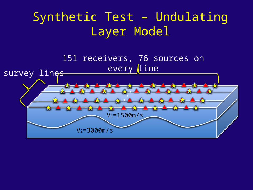
Synthetic Test – Undulating Layer Model

••

•

V1=1500m/s

V2=3000m/s

151 receivers, 76 sources on every line

11 survey lines

Line1

Line11Synthetic Result •••

Original data Data with random noise

Super-virtual refraction Iterative Super-virtual RefractionTrace

Time (s)

0

31 151 Trace

Time (s)

0

31 151

Trace

Time (s)

0

31 151 Trace

Time (s)

0

31 151

Outline

• Motivation: from 2D to 3D• Theory: conventional SVI with stationary

phase integration• Synthetic data example• Field data example• Conclusion• Acknowledgement

19

x [km]

y [k

m]

2 14

-2

18

3D OBS Survey Geometry

400 m

50 m50 m

5 m

• Sihil 3D OBS data– 234 OBS stations– 129 source-lines

• Irregular geometry.

Map view

Field Results 1Raw data

Band-pass filtered data Super-virtual resultTrace

Time (s)

0

41 361

Trace

Time (s)

0

41 361 Trace

Time (s)

0

41 361

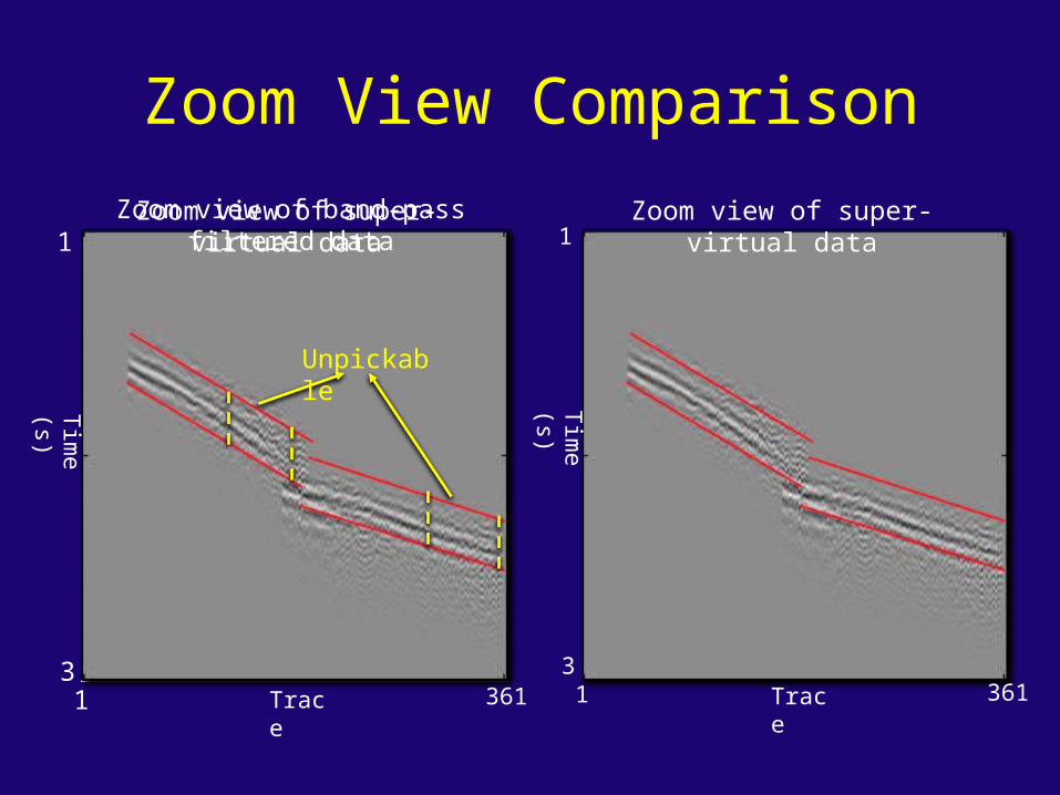
Zoom View ComparisonZoom view of band-pass filtered data Zoom view of super-virtual data

Trace

Time (s)

1

31 361 Trace

Time (s)

1

31 361

Zoom view of super-virtual data

Unpickable

Field Results 2Raw data

Super-virtual result Iterative Super-virtual resultTrace

Time (s)

0

41 361

Trace

Time (s)

0

41 361 Trace

Time (s)

0

41 361

Zoom View ComparisonRaw data

Super-virtual result Iterative Super-virtual resultTrace

Time (s)

0

41 361

Trace

Time (s)

0

41 361 Trace

Time (s)

0

41 361

Unpickable

Unpickable

Outline

• Introduction and Motivation• Theory: conventional SVI with stationary

phase integration• Synthetic data example• Field data example• Conclusion• Acknowledgement

Conclusion• We apply stationary phase integration method

to achieve super-virtual refraction with enhanced SNR in 3D cases.

• Iterative method is an option to further improve SNR when super-virtual refraction is still noisy.

• Artifacts can be produced because of the limited aperture for integration as well as a coarse spacing of sources or receivers.

Thank you !