3D Static Modelling of Pliocene reservoir, Buselli field...

IJISET - International Journal of Innovative Science, Engineering & Technology, Vol. 3 Issue 1, January 2016.

www.ijiset.com

ISSN 2348 – 7968

3D Static Modelling of Pliocene reservoir, Buselli field, Onshore Nile Delta, Egypt.

M. Y. Zein El-Din P

1P, Nabil Abdel Hafez P

2P and Osama Mahrous P

3

[email protected] Professor of petroleum exploration, Geology department, Al Azhar University, Cairo, EgyptP

1

Professor of geology, Geology department, Al Azhar University, Cairo, EgyptP

2 Senior Geologist, DEA Egypt Co., Cairo, EgyptP

3 29TABSTRACT29T:. The Buselli field is Tertiary structure in the lower Pliocene and middle Miocene. The lower Pliocene structure is four way closures bounded by two faults. A giant Abu Qir gas field is the analogue for Buselli gas discovery and the objective is to test similar structure and stratigraphy trap. The objective is to find the potentiality of Pliocene interval and the expected Facies geometry with facies distribution along the field laterally and vertically. as well as provide a dry hole analysis and explanation for El- Hessa exploratory well, however structurally was drilled in up dip comparing to Buselli discovery well, The Pliocene static model was generated using seismic sequence stratigraphy. This technique has been used for picking and tracing seismic reflectors in Pliocene interval in Nile delta. Seismic data for Buselli field reflect a good quality data and its provide one of most important input to define and predict reservoir facies distribution away from well control, using the 3D seismic cubes enables to quantify the distribution of each facies type in the total volume for reservoir calculation., 3D inverted seismic cubes were used to reduce risk associated with facies modelling and associated petrophysical properties. 29TKEYWORDS29T: Nile Delta, sequence stratigraphy, 3D Reservoir model, Seismic, inversion.

INTRODUCTION Buselli field is located onshore Nile Delta about 20 km east of Abu Qir gas field (Fig.1) and some 6 km south of

Rosetta town. Buselli well was drilled by Phillips Oil Company in 1970 with total depth 2693.5 m at Qawasim Formation. At that time it did not represent any economic value. The Buselli structure is a Tertiary structure of lower Pliocene and middle Miocene. The lower Pliocene Structure is a four way dip closure while the Miocene one is a dependent faults closure. The well objective was to test similar structure and stratigraphy in nearby productive Abu Qir gas field. The first target was Abu Madi reservoir which was considered to be well developed north of the Hinge line zone. Also by drilling Buselli well some information will be gained between the wells to the south and to the north and east (Abu Qir and IEOC wells).

The well tested gas bearing sand in Kafr El Sheikh Formation as a good secondary target while the first target

Abu Madi sand proved to be dry. The natural gas was produced from Buselli well at 5300 ft. probably it originated in Kafr El Sheikh Shale; (strong background reading of methane in mud seems to indicate that shale of the northern delta wells (Abu Qir-1x and Buselli -1x) have a good source potential. The pressures indicated that gas was probably produced from sand lens rather than blanket sand, and the closure may be a result of uncertain east west fault.

405

http://www.ijiset.com/


www.ijiset.com

ISSN 2348 – 7968

Figure 1: Buselli well location map

GEOLOGICAL SETTING The Nile delta plays a key role in tectonic evolution of eastern Mediterranean and Levant basin. It lies on the

northern margin with the African plate which extends from the subduction zone adjacent to the Cretan and Cyprus arcs

to the red sea, where it is rifted apart from the Arabian plate. (EGPC, 1984). Structure and deposition are controlled

since Eocene time by vertical movement associated with gradual sinking of the Mediterranean basin and opening of red

sea rift. In addition, the faulting northern coast to Cyrenaica was probably coincident with opening of Gulf of Suez.

An ancestral Nile delta broke into the present delta region in middle –late Miocene. However deltaic progrdation

started in late Pliocene and developed in the Pleistocene. The area of greater Nile delta can be divided from south to

north into four structural sedimentary provinces (Sestini, 1989); the South Delta Province, the North Delta Province,

the Nile Cone and the Levant Platform.

Fig. 2: Main structure elements on Nile Delta (after RWE Dea)

406



www.ijiset.com

ISSN 2348 – 7968

The main feature in delta area is the faulted flexure zone or the hinge line zone (Fig.2), which tectonically affects

pre Miocene formations and extends East -West across the middle onshore part area producing step faults Its age was

dated back to a Jurassic crustal break and about 30-40 km width, representing the boundary between a southern stable

platform and a northern subsided basin.

. The hinge zone has played a dominant role in the stratigraphic and tectonic evolution of the Nile Delta (Said,

1981; Herms and Wary, 1990). North of hinge zone Cretaceous-Middle Eocene carbonate platform drops to the north

with facies changes between platform and slope carbonates that form the westward continuation of the Jurassic-

Cretaceous hinge zone of the north Sinai and Palestine (EGPC, 1994).To the north of the hinge zone there is the

dominant positive structures Abu Madi anticline which appear to correspond to paleo-relief on the Messinian

unconformity surface.

Discussion

The well database comprises Busille-1x and El-Hessa wells with available input data from Wire line logs,

lithology log , petrophysical ELAN analysis, geological well picks .The seismic interpretation of Structure maps

(times, and depth) and fault sticks. 3D seismic amplitude data with Inversion cube used to predict the facies

distribution.

STATIC MODEL USING CORNER POINT GRIDDING Corner point gridding is classical process for making a structural model in Petrel.. The Corner point gridding

process in Petrel is subdivided into three steps: Fault modelling, pillar gridding and make horizon. Fault modelling

starts by defining which faults should be modelled as basis for generating the 3D grid. The Problems with the fault

model are often not appearing till Pillar gridding step, and problems with the pillar grid may not be obvious before

starting to build the surfaces with Make horizons.

Fault modelling

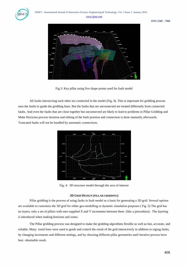
The fault model was built using fault sticks as resulting from seismic interpretation. The faults are named from

fault 1 to fault-13.These faults are used to create structure fault model using key pillars. A key pillar is a vertical, linear,

or curved line described by two, three or five shape points. Two for vertical and linear while three and more for curved

shape. Several key pillars (Fig.3) joined together by these shape points define the fault plane. Fault modelling is the

first step and the key Pillars build along all the faults to incorporate them into the reservoir model. The Fault modelling

process in conjunction with the Pillar griddling process is an iterative process used to solve some Pillar gridding

problems.

407



www.ijiset.com

ISSN 2348 – 7968

Fig.3: Key pillar using five shape points used for fault model

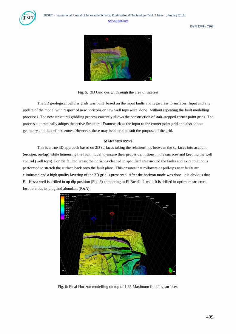
All faults intersecting each other are connected in the model (Fig. 4). This is important for gridding process

uses the faults to guide the gridding lines. But the faults that are unconnected are treated differently from connected

faults. And even the faults that are close together but unconnected are likely to lead to problems in Pillar Gridding and

Make Horizons process iteration and editing of the fault position and connection is done manually afterwards.

Truncated faults will not be handled by automatic connections.

Fig. 4: 3D structure model through the area of interest

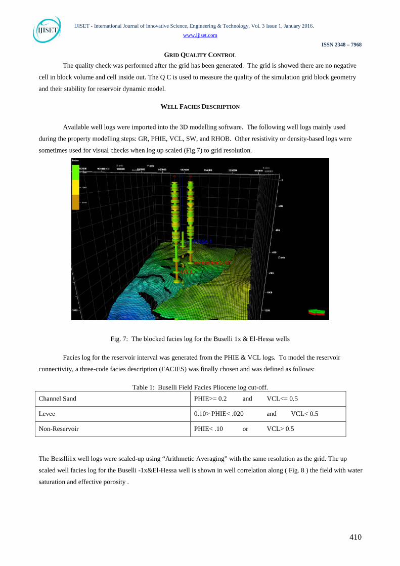
3D GRID DESIGN (PILLAR GRIDDING) Pillar gridding is the process of using faults in fault model as a basis for generating a 3D grid. Several options

are available to customize the 3D grid for either geo-modelling or dynamic simulation purposes ( Fig. 5) The grid has

no layers, only a set of pillars with user-supplied X and Y increments between them (like a pincushion) . The layering

is introduced when making horizons and zones.

The Pillar gridding process was designed to make the gridding algorithms flexible as well as fast, accurate, and

reliable. Many trend lines were used to guide and control the result of the grid interactively in addition to zigzag faults,

by changing increments and different settings, and by choosing different pillar geometries until iterative process have

best obtainable result.

408



www.ijiset.com

ISSN 2348 – 7968

Fig. 5: 3D Grid design through the area of interest

The 3D geological cellular grids was built based on the input faults and regardless to surfaces .Input and any

update of the model with respect of new horizons or new well tops were done without repeating the fault modelling

processes. The new structural gridding process currently allows the construction of stair-stepped corner point grids. The

process automatically adopts the active Structural Framework as the input to the corner point grid and also adopts

geometry and the defined zones. However, these may be altered to suit the purpose of the grid.

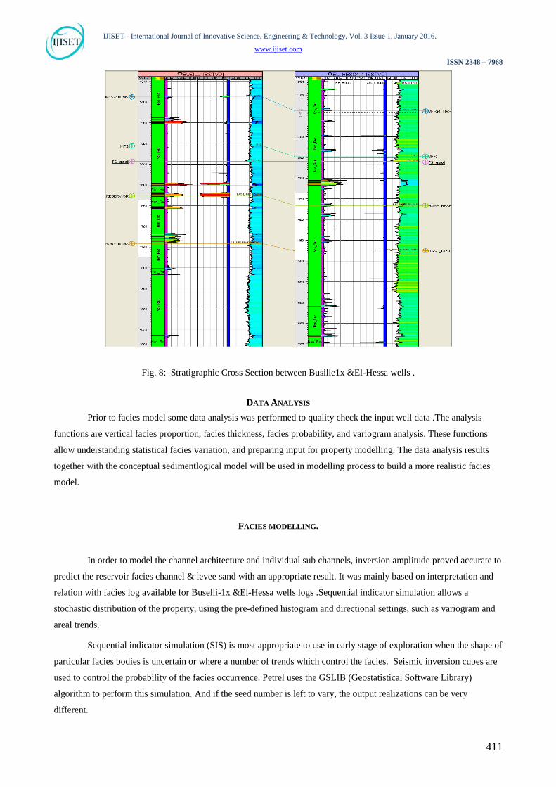
MAKE HORIZONS This is a true 3D approach based on 2D surfaces taking the relationships between the surfaces into account

(erosion, on-lap) while honouring the fault model to ensure their proper definitions in the surfaces and keeping the well

control (well tops). For the faulted areas, the horizons cleaned in specified area around the faults and extrapolation is

performed to stretch the surface back onto the fault plane. This ensures that rollovers or pull-ups near faults are

eliminated and a high quality layering of the 3D grid is preserved. After the horizon mode was done, it is obvious that

El- Hessa well is drilled in up dip position (Fig. 6) comparing to El Buselli-1 well. It is drilled in optimum structure

location, but its plug and abundant (P&A).

Fig. 6: Final Horizon modelling on top of 1.63 Maximum flooding surfaces.

409



www.ijiset.com

ISSN 2348 – 7968

GRID QUALITY CONTROL The quality check was performed after the grid has been generated. The grid is showed there are no negative

cell in block volume and cell inside out. The Q C is used to measure the quality of the simulation grid block geometry

and their stability for reservoir dynamic model.

WELL FACIES DESCRIPTION

Available well logs were imported into the 3D modelling software. The following well logs mainly used

during the property modelling steps: GR, PHIE, VCL, SW, and RHOB. Other resistivity or density-based logs were

sometimes used for visual checks when log up scaled (Fig.7) to grid resolution.

Fig. 7: The blocked facies log for the Buselli 1x & El-Hessa wells

Facies log for the reservoir interval was generated from the PHIE & VCL logs. To model the reservoir

connectivity, a three-code facies description (FACIES) was finally chosen and was defined as follows:

Table 1: Buselli Field Facies Pliocene log cut-off.

Channel Sand PHIE>= 0.2 and VCL<= 0.5

Levee 0.10> PHIE< .020 and VCL< 0.5

Non-Reservoir PHIE< .10 or VCL> 0.5

The Besslli1x well logs were scaled-up using “Arithmetic Averaging” with the same resolution as the grid. The up

scaled well facies log for the Buselli -1x&El-Hessa well is shown in well correlation along ( Fig. 8 ) the field with water

saturation and effective porosity .

410



www.ijiset.com

ISSN 2348 – 7968

Fig. 8: Stratigraphic Cross Section between Busille1x &El-Hessa wells .

DATA ANALYSIS Prior to facies model some data analysis was performed to quality check the input well data .The analysis

functions are vertical facies proportion, facies thickness, facies probability, and variogram analysis. These functions

allow understanding statistical facies variation, and preparing input for property modelling. The data analysis results

together with the conceptual sedimentlogical model will be used in modelling process to build a more realistic facies

model.

FACIES MODELLING.

In order to model the channel architecture and individual sub channels, inversion amplitude proved accurate to

predict the reservoir facies channel & levee sand with an appropriate result. It was mainly based on interpretation and

relation with facies log available for Buselli-1x &El-Hessa wells logs .Sequential indicator simulation allows a

stochastic distribution of the property, using the pre-defined histogram and directional settings, such as variogram and

areal trends.

Sequential indicator simulation (SIS) is most appropriate to use in early stage of exploration when the shape of

particular facies bodies is uncertain or where a number of trends which control the facies. Seismic inversion cubes are

used to control the probability of the facies occurrence. Petrel uses the GSLIB (Geostatistical Software Library)

algorithm to perform this simulation. And if the seed number is left to vary, the output realizations can be very

different.

411



www.ijiset.com

ISSN 2348 – 7968

In this study the reservoir facies geometry was observed from seismic data to provide valuable information

used in modelling process. stochastic facies including high quality connected channel and associated levees distributed

using particular algorithm SIS and guided by 3D inversion seismic cubes. For facies model using 3D seismic data two

products of AVO inversion cubes were used. Impedance and the Poisson's ratio are used to allocate sand bodies. In

Buselli field it was necessary to have absolute dimension for reservoir elements .But limited well data, and lack of core

and sedimentary study give more weight to seismic data which give an image for individual channel within Buselli

field, width, sinuosity, amplitude and azimuth. The facies probability function was used to help the modelling software

to accurately locate reservoir facies based on seismic data. The Poisson's ratio cubes is the geophysical measure of rock

properties, density and saturation with direct relation to reservoir properties and facies, so the inversion cubes hav been

analyzed and correlated statistically to facies log and resulted function from relation between facies and seismic as

facies probability plot.

A detailed rock physics analysis was conducted using the extensive log suites from the existing wells. The

sandstone reservoirs are Pliocene, deposited as channel sands and levees. The range of the PR and VP/Vs were taken

from facies probability function to help the modelling software to accurately locate reservoir facies based on seismic

data.

During the modelling Petrel software start to look for seismic cubes in all cells simultaneously. With

probability function (Fig .9 ) when a particular seismic value indicates specific facies rock type, the software populates

the cell with this seismic value by this facies rock code type

Fig. 9: Facies probability function of Facies with poisson ratio attributes

The Pliocene zone at well location indicates limited sand facies and high shale content. The facies model

conditioned to inversion seismic data shows that the channel direction North West south east and running along Buselli

well and at the location of El Hessa was not drilled in optimum location along the channel and there is fairway sand

distribution into northern direction (Fig. 10)

412



www.ijiset.com

ISSN 2348 – 7968

Fig. 10: Sequential indicator simulation Facies model conditioned to poisson ratio

Also Pliocene zone shows Relationship between a discrete property facies log and secondary seismic attribute

Using Vp/ Vs with facies log in probability function curve is used to define a different Facies scenario

(Fig.11).This relationship shows that more levees sediments have been deposited associated with channel and splay.

Fig. 11: Facies probability function of Facies with Vp Vs ratio attributes

Using 3D volume trend to guide the Pliocene sand distribution, this trend has been noticed from seismic

attribute map. Assuming that sand deposited as channel trending NW-SE direction controlled by main bounding fault

(Fig.12).

413



www.ijiset.com

ISSN 2348 – 7968

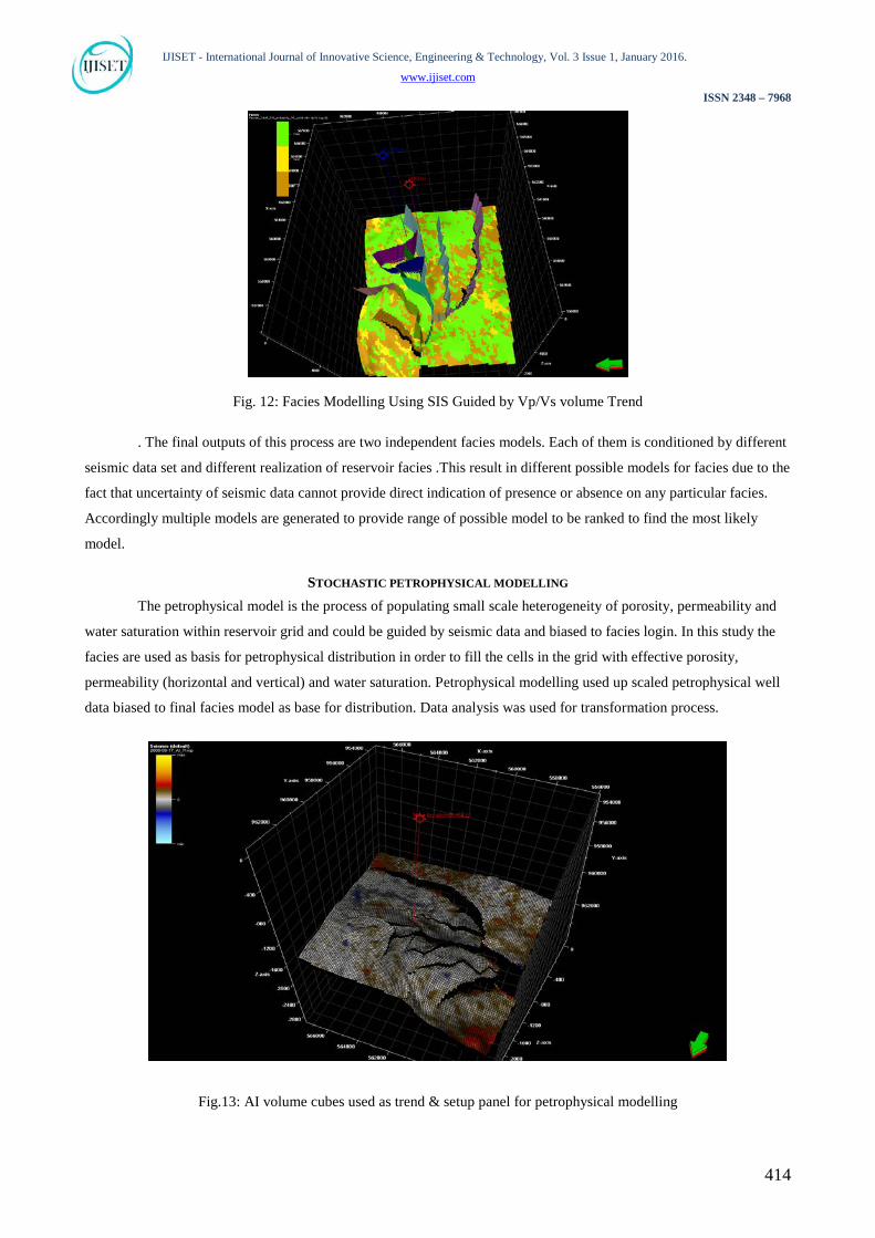
Fig. 12: Facies Modelling Using SIS Guided by Vp/Vs volume Trend

. The final outputs of this process are two independent facies models. Each of them is conditioned by different

seismic data set and different realization of reservoir facies .This result in different possible models for facies due to the

fact that uncertainty of seismic data cannot provide direct indication of presence or absence on any particular facies.

Accordingly multiple models are generated to provide range of possible model to be ranked to find the most likely

model.

STOCHASTIC PETROPHYSICAL MODELLING The petrophysical model is the process of populating small scale heterogeneity of porosity, permeability and

water saturation within reservoir grid and could be guided by seismic data and biased to facies login. In this study the

facies are used as basis for petrophysical distribution in order to fill the cells in the grid with effective porosity,

permeability (horizontal and vertical) and water saturation. Petrophysical modelling used up scaled petrophysical well

data biased to final facies model as base for distribution. Data analysis was used for transformation process.

Fig.13: AI volume cubes used as trend & setup panel for petrophysical modelling

414



www.ijiset.com

ISSN 2348 – 7968

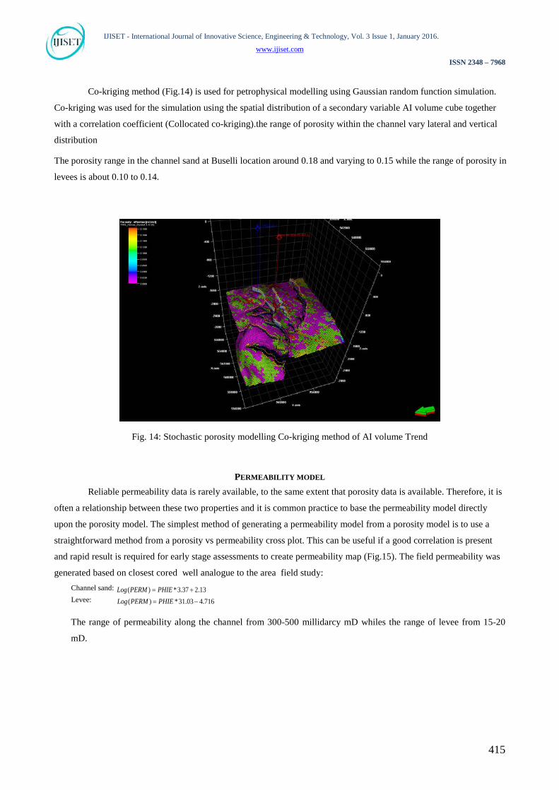
Co-kriging method (Fig.14) is used for petrophysical modelling using Gaussian random function simulation.

Co-kriging was used for the simulation using the spatial distribution of a secondary variable AI volume cube together

with a correlation coefficient (Collocated co-kriging).the range of porosity within the channel vary lateral and vertical

distribution

The porosity range in the channel sand at Buselli location around 0.18 and varying to 0.15 while the range of porosity in

levees is about 0.10 to 0.14.

Fig. 14: Stochastic porosity modelling Co-kriging method of AI volume Trend

PERMEABILITY MODEL Reliable permeability data is rarely available, to the same extent that porosity data is available. Therefore, it is

often a relationship between these two properties and it is common practice to base the permeability model directly

upon the porosity model. The simplest method of generating a permeability model from a porosity model is to use a

straightforward method from a porosity vs permeability cross plot. This can be useful if a good correlation is present

and rapid result is required for early stage assessments to create permeability map (Fig.15). The field permeability was

generated based on closest cored well analogue to the area field study: Channel sand: 13.237.3*)( += PHIEPERMLog Levee: 716.403.31*)( −= PHIEPERMLog The range of permeability along the channel from 300-500 millidarcy mD whiles the range of levee from 15-20

mD.

415



www.ijiset.com

ISSN 2348 – 7968

Fig. 15: Permeability modelling based on direct relation with 3D porosity model

SATURATION MODEL For volumetric calculation estimate the saturation (Fig.16) of Pliocene reservoir have been created with

stochastic approach in each reservoir Facies types. Average channel saturation = .015 and average levee saturation =

0.45 and in sensitivity analysis the saturation parameter will be given different range with different percentage facies

rock type.

Fig. 16: Water Saturation modelling based on direct relation with 3D porosity model

FACIES CONNECTIVITY

Buselli reservoir is considered as multi reservoir channels and associated levee, the

connectivity property (Fig.17) parameter is defined the connected sand body laterally and vertically.

416



www.ijiset.com

ISSN 2348 – 7968

Fig. 17: Cross section shows the Facies connectivity along Buselli field

CONCLUSION The Pliocene static model is used to define potentiality of Buselli field, Buselli reservoir is considered as multi

reservoir channels and associated levee, the connectivity property parameter is defined the connected sand body laterally and vertically. With levees, the connected facies gives clear indication of potentiality in the Buselli field. This will help to estimate the numbering of wells and amount of reservoir to be penetrated by proposal wells. However Hessa well was not drilled in the optimum location and drilled off the channel belt. Pliocene static model confirm presence of new upside potential in Buselli Field. The use of conditional Reservoir model is reduced the associated exploration risk around the field.

REFERENCES Robertson, 1983; Hull, 1988): Robertson, A.H.F., Dixon, J.E., 1984. Introduction: aspects of the geological evolution of the Eastern Mediterranean. In: Dixon,J.E., Robertson, A.H.F. (Eds.), The Geological Evolution of the Eastern Mediterranean, Geological Society Special Publication,vol. 17, pp. 1 –74. Sestini, G. (1989): Geomorphology of the Nile Delta: Proceedings of seminar on Nile Delta sedimentology. UNESCO/ASR/UNDP. Alexandria. Said, 1981; Herms and Wary, 1990: stratigraphic and tectonic evolution of the Nile Delta

Said, R. (1981): The geological Evolution of the River Nile -Springer, 151pp.Texas, USA.. Schlumberger (1984): Geology of Egypt pp.1-64. - Paper presented at the Well Evaluation Conference, Schlumberger, and Cairo.

Sestini, G. (1989): Geomorphology of the Nile Delta: Proceedings of seminar on Nile Delta sedimentology. UNESCO/ASR/UNDP. Alexandria. Schlumberger (2010): Petrel user manual for property distribution.

417


3D Static Modelling of Pliocene reservoir, Buselli field...

Documents

Transcript of 3D Static Modelling of Pliocene reservoir, Buselli field...