TO DOWNLOAD A COPY OF THIS POSTER, VISIT WWW.WATERS.COM/POSTERS ©2013 Waters Corporation

OVERVIEW

We present numerical simulation of ions from a gas cell through an exit aperture and into a quadrupole mass filter

The method includes simulation of gas flow through the exit aperture and modelling of the quadrupole entrance fringe fields in 3D

We find generally good agreement between the simulated results and experimental data from a tandem quadrupole instrument

INTRODUCTION

The quadrupole mass filter (QMF) is widely used as a mass

analyser. Numerical simulation of quadrupole mass filter performance is demanding owing to a number of factors:

Highly accurate fields are required to correctly determine

stable ion trajectories through the filter.

Ion motion is strongly affected by the entrance fringe fields,

hence the fields must be solved in 3D.

Ion motion is strongly dependent on the initial conditions of

the ions on entry to the quadrupole.

Due to these difficulties prior quadrupole simulations were

often restricted to 2D fields, with approximations used for the 3D fringe fields and for the initial ion distributions. While such

2D calculations often show good general agreement with experimental results they are rarely quantitatively accurate.

Owing to recent advances in computing power and numerical

methods it is now feasible to fully simulate QMFs in 3D on typical desktop computers. In this poster we present the

simulation of ions from a stacked ring ion guide (SRIG)

through an aperture plate into a quadrupole mass filter. Figure 1 shows a schematic of the geometry used for the

simulation, corresponding to the collision cell and second analyser in a tandem quadrupole mass spectrometer.

3D SIMULATION OF QUADRUPOLE MASS FILTER PERFORMANCE WITH REALISTIC ION INPUT CONDITIONS

David Langridge

Waters Corporation, Manchester, UK

METHODS

Simulation

Ions are created in the SRIG gas cell and are driven towards the exit aperture by a low amplitude T-Wave. To speed up

repeated calculations the ions are recorded at a plane near the exit end of the SRIG gas cell, these ion initial conditions can

then be re-used for further calculations where we have the same ion mass/charge and SRIG gas cell settings. The SRIG

gas cell is typically at 2.6e-3 torr while the quadrupole analyser is at 1.9e-5 torr. Gas flow through the exit aperture

was modeled using the Direct Simulation Monte-Carlo (DSMC) method [1], hence in the region of the exit aperture we have

variation in the pressure, temperature and velocity of the

background gas. Figure 2 shows an example of the calculated pressure and axial gas velocity distributions. A hard sphere

collision model was used for the interaction of the ions with the background gas.

References

1. G. A. Bird, Molecular Gas Dynamics and the Direct Simulation of Gas Flows (Oxford University Press, Oxford, 1994).

2. SIMION 3D v8.1, Scientific Instrument Services Ltd.

3. Gibson, J.R., Evans, K.G., Sarfaraz U.S., Maher S., Taylor, S.: A Method of Computing Accurate 3D Fields of a Quadrupole Mass Filter and Their Use for Prediction of Filter Behavior. J. Am. Soc. Mass. Spectrom. 23, 1593–1601 (2012)

RESULTS

Figure 4 plots the experimental and simulated resolution vs

transmission curves for singly charged ions of m/z 175, 556

and 732, with the ion energy set at 10eV (i.e. a 10V DC drop from the SRIG to the quadrupole). Transmission is given as a

percentage of the peak height vs the unresolved peak height, resolution is calculated as m/ m where m is the FWHM of

the peak.

The results are in relatively good agreement. For the m/z 175 ion the simulated results give 10-15% higher transmission at a

given resolution, while m/z 556 and 732 are in very good agreement except at the higher resolution settings where the

experimental results tend to drop in transmission. This is not unexpected as any mechanical or electrical imperfections in

the quadrupole field will limit the physical system as we narrow the transmission window at the apex of the stability

diagram. There is considerable scatter in the experimental

results since we cannot acquire resolved and unresolved data simultaneously, we have to compare consecutive acquisitions

leading to possible errors if the signal intensity varies.

Figure 5 plots the experimental and simulated peaks for the 10eV m/z 556 ion at two resolution settings (about 650 and

1400 m/ m). The peak height and resolution are consistent as

shown in the previous plot, however we can also see that the

peak shape is almost identical between the experimental data and the simulation. Given that there are no empirical

corrections applied to the simulated data (beyond correction for the mass position on the mass scale) this level of

agreement is very encouraging.

10eV is significantly higher than the usual operating ion energy of a tandem quadrupole, hence the resolution is quite poor and

the peak shapes have large tails. At 10eV we might expect

small variations in the actual experimental ion energy and any on-axis RF effects to be minimised relative to the high ion

energy, thus there is likely to be better agreement between experiment and simulation.

CONCLUSION

We demonstrate simulation of ion motion from a gas

cell into a quadrupole mass filter

Generally good agreement between experiment and

simulation, although further work is required to determine the source of discrepancies

Allows rapid prototyping of new analyser designs

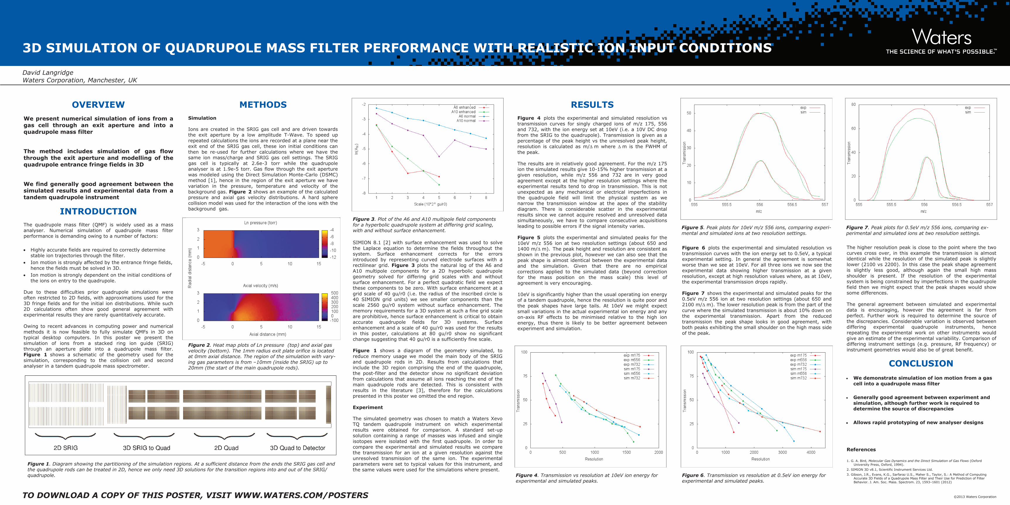
Figure 3. Plot of the A6 and A10 multipole field components

for a hyperbolic quadrupole system at differing grid scaling, with and without surface enhancement.

Figure 1. Diagram showing the partitioning of the simulation regions. At a sufficient distance from the ends the SRIG gas cell and

the quadrupole rods can be treated in 2D, hence we only need 3D solutions for the transition regions into and out of the SRIG/quadrupole.

Figure 2. Heat map plots of Ln pressure (top) and axial gas

velocity (bottom). The 1mm radius exit plate orifice is located at 0mm axial distance. The region of the simulation with vary-

ing gas parameters is from –10mm (inside the SRIG) up to 20mm (the start of the main quadrupole rods).

SIMION 8.1 [2] with surface enhancement was used to solve

the Laplace equation to determine the fields throughout the system. Surface enhancement corrects for the errors

introduced by representing curved electrode surfaces with a rectilinear grid. Figure 3 plots the natural log of the A6 and

A10 multipole components for a 2D hyperbolic quadrupole geometry solved for differing grid scales with and without

surface enhancement. For a perfect quadratic field we expect these components to be zero. With surface enhancement at a

grid scale of 40 gu/r0 (i.e. the radius of the inscribed circle is 40 SIMION grid units) we see smaller components than the

scale 2560 gu/r0 system without surface enhancement. The memory requirements for a 3D system at such a fine grid scale

are prohibitive, hence surface enhancement is critical to obtain accurate quadrupole fields for 3D systems. Surface

enhancement and a scale of 40 gu/r0 was used for the results

in this poster, calculations at 80 gu/r0 show no significant change suggesting that 40 gu/r0 is a sufficiently fine scale.

Figure 1 shows a diagram of the geometry simulated, to

reduce memory usage we model the main body of the SRIG and quadrupole rods in 2D. Results from calculations that

include the 3D region comprising the end of the quadrupole, the post-filter and the detector show no significant deviation

from calculations that assume all ions reaching the end of the main quadrupole rods are detected. This is consistent with

results in the literature [3], therefore for the calculations presented in this poster we omitted the end region.

Experiment

The simulated geometry was chosen to match a Waters Xevo TQ tandem quadrupole instrument on which experimental

results were obtained for comparison. A standard set-up solution containing a range of masses was infused and single

isotopes were isolated with the first quadrupole. In order to compare the experimental and simulated results we compare

the transmission for an ion at a given resolution against the unresolved transmission of the same ion. The experimental

parameters were set to typical values for this instrument, and the same values were used for the simulations where present.

Figure 4. Transmission vs resolution at 10eV ion energy for

experimental and simulated peaks.

Figure 6. Transmission vs resolution at 0.5eV ion energy for

experimental and simulated peaks.

Figure 6 plots the experimental and simulated resolution vs

transmission curves with the ion energy set to 0.5eV, a typical experimental setting. In general the agreement is somewhat

worse than we see at 10eV. For all three ions we now see the experimental data showing higher transmission at a given

resolution, except at high resolution values where, as at 10eV, the experimental transmission drops rapidly.

Figure 7 shows the experimental and simulated peaks for the

0.5eV m/z 556 ion at two resolution settings (about 650 and 2100 m/ m). The lower resolution peak is from the part of the

curve where the simulated transmission is about 10% down on the experimental transmission. Apart from the reduced

transmission the peak shape looks in good agreement, with both peaks exhibiting the small shoulder on the high mass side

of the peak.

Figure 5. Peak plots for 10eV m/z 556 ions, comparing experi-

mental and simulated ions at two resolution settings.

Figure 7. Peak plots for 0.5eV m/z 556 ions, comparing ex-

perimental and simulated ions at two resolution settings.

The higher resolution peak is close to the point where the two

curves cross over, in this example the transmission is almost identical while the resolution of the simulated peak is slightly

lower (2100 vs 2200). In this case the peak shape agreement is slightly less good, although again the small high mass

shoulder is present. If the resolution of the experimental system is being constrained by imperfections in the quadrupole

field then we might expect that the peak shapes would show some differences.

The general agreement between simulated and experimental

data is encouraging, however the agreement is far from perfect. Further work is required to determine the source of

the discrepancies. Considerable variation is observed between differing experimental quadrupole instruments, hence

repeating the experimental work on other instruments would

give an estimate of the experimental variability. Comparison of differing instrument settings (e.g. pressure, RF frequency) or

instrument geometries would also be of great benefit.