
3D Object Recognition and Pose with Relational Indexing
44
Computer Vision and Image Understanding 79, 364–407 (2000) doi:10.1006/cviu.2000.0865, available online at http://www.idealibrary.com on 3D Object Recognition and Pose with Relational Indexing 1 Mauro S. Costa Boeing Commercial Airplane Group, Seattle, Washington E-mail: [email protected] and Linda G. Shapiro University of Washington, Seattle, Washington E-mail: [email protected] Received September 14, 1998; accepted June 1, 2000 This paper addresses the problem of recognizing 3D objects from 2D intensity images. It describes the object recognition system named RIO (relational indexing of objects), which contains a number of new techniques. RIO begins with an edge image obtained from a pair of intensity images taken with a single camera and two different lightings. From the edge image, a set of new high-level features and relationships are extracted, and a technique called relational indexing is used to efficiently recall 2D view-class object models that have similar relational descriptions from a potentially large database of models. Once a model has been hypothesized, pairs of 2D–3D corresponding features, including point pairs, line–segment pairs, and ellipse–circle pairs, are used in a new linear pose estimation framework to produce a hypothesized transformation from a 3D mesh model of the object to the image. The transformation is either accepted or rejected by a verification procedure that projects the 3D model wireframe to the image and computes a Hausdorff-like distance measure between the projected model and the edge image. The resultant object recognition system is able to recognize 3D objects having planar, cylindrical, and threaded surfaces in complex, multiobject scenes. c 2000 Academic Press 1 This research was supported by the National Science Foundation under Grant IRI-9023977, by the Washington Technology Center, and by the Boeing Commercial Airplane Group. 364 1077-3142/00 $35.00 Copyright c 2000 by Academic Press All rights of reproduction in any form reserved.
Transcript of 3D Object Recognition and Pose with Relational Indexing
Computer Vision and Image Understanding79,364–407 (2000)doi:10.1006/cviu.2000.0865, available online at http://www.idealibrary.com on
3D Object Recognition and Posewith Relational Indexing1
Mauro S. Costa
Boeing Commercial Airplane Group, Seattle, WashingtonE-mail: [email protected]
and
Linda G. Shapiro
University of Washington, Seattle, WashingtonE-mail: [email protected]
Received September 14, 1998; accepted June 1, 2000
This paper addresses the problem of recognizing 3D objects from 2D intensityimages. It describes the object recognition system named RIO (relational indexing ofobjects), which contains a number of new techniques. RIO begins with an edge imageobtained from a pair of intensity images taken with a single camera and two differentlightings. From the edge image, a set of new high-level features and relationships areextracted, and a technique called relational indexing is used to efficiently recall 2Dview-class object models that have similar relational descriptions from a potentiallylarge database of models. Once a model has been hypothesized, pairs of 2D–3Dcorresponding features, including point pairs, line–segment pairs, and ellipse–circlepairs, are used in a new linear pose estimation framework to produce a hypothesizedtransformation from a 3D mesh model of the object to the image. The transformationis either accepted or rejected by a verification procedure that projects the 3D modelwireframe to the image and computes a Hausdorff-like distance measure betweenthe projected model and the edge image. The resultant object recognition systemis able to recognize 3D objects having planar, cylindrical, and threaded surfaces incomplex, multiobject scenes.c© 2000 Academic Press
1 This research was supported by the National Science Foundation under Grant IRI-9023977, by the WashingtonTechnology Center, and by the Boeing Commercial Airplane Group.
364
1077-3142/00 $35.00Copyright c© 2000 by Academic PressAll rights of reproduction in any form reserved.

3D OBJECT RECOGNITION AND RELATIONAL INDEXING 365
1. INTRODUCTION
Three-dimensional object recognition has seen a great deal of activity in the past decade,as has been pointed out in recent surveys [3, 6, 13, 46, 53]. Most systems fall into threemain categories: (1) systems that use intensity data alone [1, 7, 9, 11, 35, 42, 43, 48, 59],(2) systems that use range data alone [5, 10, 24, 26, 27, 38, 30, 37, 40, 50], and (3) systemsthat use both range and intensity (sometimes including color) data [31, 34, 52].
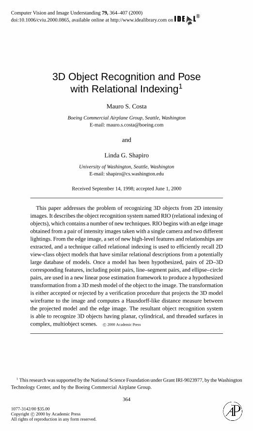
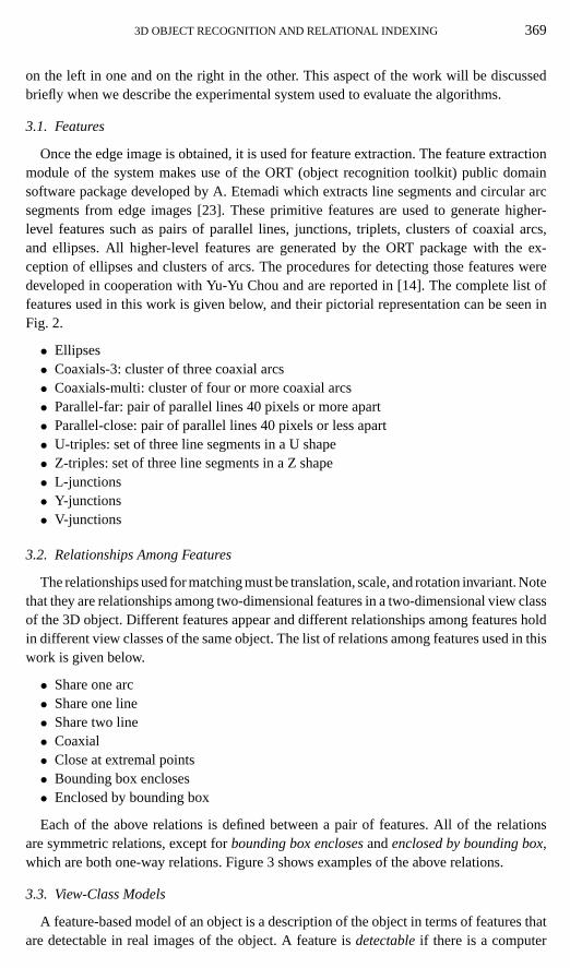
In intensity-image-based systems, points and straight line segments are still the mostcommonly-used features. In fact, the recent popularity of the alignment method [36] hasled to a significant number of systems that blindly match triples of points or line segmentsfrom the image to similar triples from the model, using little or no contextual information.These algorithms all make the assumptions that (a) the points or line segments are reasonablyreliable features of the class of objects to be recognized or located and (b) the pose of theobject can be uniquely determined from a small set of these features. These assumptions areonly true for polyhedral objects or those with a number of sharp, straight edges. They fallapart for most curved-surface objects. Figure 1a shows a polyhedral object where pointsand line segments make good features, and Fig. 1b shows another simple object with bothcurved and planar surfaces where they are not very useful. Our system can recognize objectsthat have planar, cylindrical, and threaded surfaces, and it is designed to handle occlusion.
In range-image-based systems, primitive surfaces (usually planar or quadric) are the mostcommon features, but 3D line segments and points are also used. Because surfaces fromrange data are more reliable than surface regions from grayscale, a number of systemsuse the properties of and relationships among surfaces in matching algorithms. This typeof approach has worked well for simple objects with a small number of simple surfaces.Systems that work with more complex, free-form surfaces generally look for interest pointsand perform point matching. Again, the reliable detection of feature points is crucial tosuccess. The recent work of Johnson and Hebert [40] provides a new and powerful way tohypothesize point correspondences.
This work addresses the problem of recognizing 3D objects from 2D intensity images. Itdescribes the object recognition system named RIO (relational indexing of objects), which
FIG. 1. (a) Image of a polyhedral object whose junctions and line segments make useful features for recognitionand pose estimation. (b) Image of a nonpolyhedral object for which line segments and junctions alone are virtuallyuseless as recognition features.
366 COSTA AND SHAPIRO
performs feature-based alignment and contains a number of new techniques. RIO beginswith an edge image obtained from a pair of intensity images taken with a single camera andtwo different lightings. From the edge image, a set of new high-level features and relation-ships are extracted, and a technique calledrelational indexingis used to efficiently recall2D view-class object models that have similar relational descriptions from a potentiallylarge database of models. Once a model has been hypothesized, pairs of 2D–3D corre-sponding features, including point pairs, line–segment pairs, and ellipse–circle pairs, aresimultaneously used in a new linear pose estimation framework to produce a hypothesizedtransformation from a 3D mesh model of the object to the image. The transformation isoptimized (and subsequently accepted or rejected) by a verification procedure that projectsthe 3D model wireframe onto the image and minimizes a Hausdorff-like distance measurebetween the projected model and the image edges. The resultant object recognition systemis able to recognize 3D objects having planar, cylindrical, and threaded surfaces in complex,multiobject scenes.
This paper describes the major research contributions of the RIO system. Section 2 dis-cusses the related literature. Section 3 defines the features and relations used for recognition.Section 4 gives the relational indexing algorithm and some initial experiments. Section 5describes the new pose-estimation algorithm, and Section 6 discusses the full experimentsand results.
2. RELATED WORK
This section briefly describes a few existing systems which are closely related to thesystem developed in this work. Whenever possible, an attempt has been made to compareor relate characteristics of the system being described to the philosophical aspects of thework described in this paper.
Features can be predicted analytically or by applying graphics software to CAD models[9, 29, 30, 56]. In [30], Gremban and Ikeuchi use the term appearance-based vision to referto methods in which the recognition system analyzes and predicts the appearances of theobject models based on CAD data and on physical sensor models. The prediction can beeither analytical or based on synthesized images of the objects in the model database. Thepredicted appearance is the set of features that are visible under a specific set of viewingconditions. The analysis of the predicted appearance allows for the generation of an objectrecognition program to be used in the online phase of the recognition process. This processis also called VAC (vision algorithm compiler), because it takes a set of object and sensormodels and outputs an executable object recognition program. The framework is general inthe sense that it does not require any specific type of sensor. Their system has successfullyrecognized simple objects from range data in a bin-picking environment. However, there aretwo drawbacks to this approach: (1) analytical prediction is impractical in some domains;and (2) synthetic images are not yet realistic enough for general use. More recently, Doraiand Jain [22] have developed a method of view grouping for free from objects, using rangeimages.
The use of synthetic images also affected the performance of the PREMIO system ofCampset al. [9]. This system utilizes artificially rendered images to predict object appear-ances under various environmental conditions (sensor, lighting, and viewpoint location).The predictions generated by the system did not agree well with the real images acquiredunder the same set of conditions. In order to improve PREMIO’s predictions, Pulli [47]
3D OBJECT RECOGNITION AND RELATIONAL INDEXING 367
developed the TRIBORS system. He initially attempted to improve the predictions by us-ing a better ray tracer, but that was also insufficient. The solution he found was to bootstrapthe prediction process with synthetic images and to train on real images. These new pre-dictions led to better and faster object recognition. The use of real training images seems tobe a step in the right direction. In this paper, the “predictions” are derived exclusively fromreal images of the objects. These predictions are described in detail in Section 2.
Despite the fact that it only deals with two-dimensional objects, Bolles and Cain’s local-feature-focus method [4] is very relevant to the work herein. Their method automaticallyanalyzes the object models and selects the best features for recognition. Typical featuresinclude holes and corners. The basic principle is to locate one relatively reliable feature anduse it to partially define a coordinate system within which a group of other key features islocated. If enough of these secondary features are located and if they can uniquely identifythe focus feature, then the hypothesized position and orientation of the object (of which thisfeature is a part) is determined. A verification step that utilizes template matching is thenperformed to prove or disprove the hypothesis. The system has been proven to efficientlyrecognize and locate a large class of partially visible two-dimensional objects.
The work of Murase and Nayar [43] also involves appearance of objects and the trainingis performed on real images. They argue that since the appearance of an object is dependenton its shape, its reflectance properties, its pose in the scene, and the illumination conditions,the problem of recognizing objects from brightness images is more a problem of appearancematching than of shape matching. They define a compact representation of object appearancethat is parameterized by pose and illumination only, since shape and reflectance are intrinsic(constant) properties. This representation is obtained by acquiring a large set of real imagesof the objects under different lighting and pose configurations and then compressing theset into an eigenspace. A hypersurface in this space represents a particular object. Atrecognition time, the image of an object is projected onto a point in the eigenspace andthe object is recognized based on the hypersurface on which it lies. The exact location ofthe point determines the pose of the object. The major drawback of this method is that itcannot handle multiple-object scenes. Occlusion also adversely affects the performance ofthe system.
Though the work of Bergevin and Levine [2] on generic object recognition does not makeuse of the specific model-based paradigm, it is philosophically related to the work herein.They utilize coarse, qualitative models that represent classes of objects. Their work is basedon the recognition by component (RBC) theory of Biederman. The system is divided intothree main subsystems: part segmentation, part labeling, and object model matching. Thepart segmentation algorithm is boundary-based, and it is independent of the specific shape ofthe parts making up an object. The part (geon) labeling algorithm makes use of the conceptof faces to further categorize the geons into generalized solids. At the matching stage, thelabeled geons are used to index into the database of models. A measure of similarity isdefined in order to discriminate among the models. An important observation made bythe authors themselves is that it is not clear that suitable line drawings may eventually beobtained from real images. All their examples and tests have made use of ideal line drawings.
The evidence-based recognition technique proposed by Jain and Hoffman [38] defines anobject representation and a recognition scheme based on salient features in range images.The objects are represented in terms of their surfaces, boundaries, and edges. The recogni-tion scheme makes use of an evidence rulebase, which is a set of evidence conditions andtheir corresponding weights for various models in the database. The similarity between a set
368 COSTA AND SHAPIRO
of observed image features and the set of evidence conditions for a given object determineswhether there is enough evidence that the particular model is in the image. The modelfeatures must be carefully chosen in order to make possible the distinction between objectclasses.
Geometric hashing [15, 41] is a matching scheme that achieves rapid online matchingperformance via a large offline preprocessing step. In the offline database creation stepof geometric hashing, salient feature points in the object models are converted into anaffine-invariant model representation by using three points as a basis and transforming thecoordinates of the remaining points. These new coordinates are encoded and used as anentry to a hash table where the basis triplet and the model from which the coordinatescame are recorded. This is done for all possible basis triplets in the models. In the matchingstep, salient points in the image are detected, a basis triplet is chosen, and the remainingpoints are transformed with respect to this basis and are used to access the table. For eachbin accessed, votes are cast for the model-basis pairs associated with the bin. After all thepoints are used in this fashion, if a particular model-view has high enough votes, an objectmatch hypothesis is declared found. The recognition part of the system described in thispaper is accomplished by utilizing the high-level features and relationships of an objectin a paradigm called relational indexing. This indexing technique is related to the originalgeometric hashing technique, except that the database of models is indexed by encoding(without quantization) small relational graphs of features, as opposed to affine-invariantpoint coordinates. Because we use symbolic information and because the information westore is much smaller than the information required for geometric hashing, our currentimplementation uses only an array for table lookups, instead of a hash table.
The work of Stein and Medioni [50] is particularly related to our indexing scheme. Intheir structural indexing technique boundaries of objects are approximated by polygonsand groups of consecutive segments are encoded and used to index the database and toretrieve possible hypotheses. In their MULTIHASH system, Grewe and Kak [31] proposean interactive framework for learning the structure of a multiple-attribute hash table for usein the recognition and localization of 3D objects. The system makes use of both qualitativeand quantitative attributes, such as shape of a surface and color, respectively. Decision treesand uncertainty modeling are used in the construction of the hash tables, after a humantrainer shows objects to the vision system and tells the system the identities of the modelscorresponding to the several attributes considered.
The work of Chen and Stockman [12] uses a hypothesize-and-test approach to genericobject recognition. Their recognition system uses an alignment paradigm consisting of threestages: modeling, indexing, and matching. In the first stage, model aspects are constructedfor predicting the object contours visible from an arbitrary viewpoint. Model aspects andpose hypotheses are generated by the indexing module, which makes use of the conceptof “parts.” In the matching stage, verification of model hypotheses is carried out by analignment technique that makes use of Newton’s method along with a Levenberg–Marquardtminimization, to estimate or refine the object pose iteratively. The hypotheses are refutedor supported by the matching results.
3. FEATURES AND RELATIONS
The features used in this work are derived from edge images. These edge images actuallycome from a pair of intensity images taken from the same viewpoint, but with the light source
3D OBJECT RECOGNITION AND RELATIONAL INDEXING 369
on the left in one and on the right in the other. This aspect of the work will be discussedbriefly when we describe the experimental system used to evaluate the algorithms.
3.1. Features
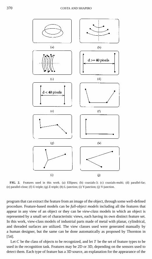
Once the edge image is obtained, it is used for feature extraction. The feature extractionmodule of the system makes use of the ORT (object recognition toolkit) public domainsoftware package developed by A. Etemadi which extracts line segments and circular arcsegments from edge images [23]. These primitive features are used to generate higher-level features such as pairs of parallel lines, junctions, triplets, clusters of coaxial arcs,and ellipses. All higher-level features are generated by the ORT package with the ex-ception of ellipses and clusters of arcs. The procedures for detecting those features weredeveloped in cooperation with Yu-Yu Chou and are reported in [14]. The complete list offeatures used in this work is given below, and their pictorial representation can be seen inFig. 2.
• Ellipses• Coaxials-3: cluster of three coaxial arcs• Coaxials-multi: cluster of four or more coaxial arcs• Parallel-far: pair of parallel lines 40 pixels or more apart• Parallel-close: pair of parallel lines 40 pixels or less apart• U-triples: set of three line segments in a U shape• Z-triples: set of three line segments in a Z shape• L-junctions• Y-junctions• V-junctions
3.2. Relationships Among Features
The relationships used for matching must be translation, scale, and rotation invariant. Notethat they are relationships among two-dimensional features in a two-dimensional view classof the 3D object. Different features appear and different relationships among features holdin different view classes of the same object. The list of relations among features used in thiswork is given below.
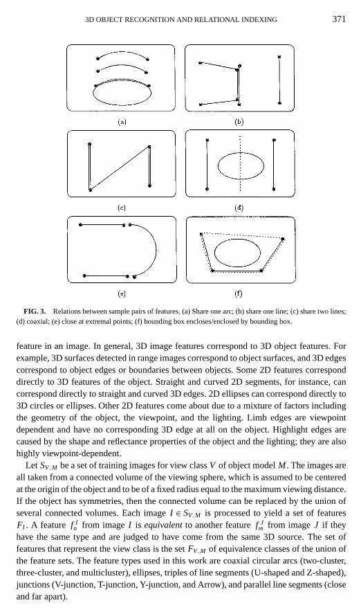
• Share one arc• Share one line• Share two line• Coaxial• Close at extremal points• Bounding box encloses• Enclosed by bounding box
Each of the above relations is defined between a pair of features. All of the relationsare symmetric relations, except forbounding box enclosesandenclosed by bounding box,which are both one-way relations. Figure 3 shows examples of the above relations.
3.3. View-Class Models
A feature-based model of an object is a description of the object in terms of features thatare detectable in real images of the object. A feature isdetectableif there is a computer
370 COSTA AND SHAPIRO
FIG. 2. Features used in this work. (a) Ellipses; (b) coaxials-3; (c) coaxials-multi; (d) parallel-far;(e) parallel-close; (f) U-triple; (g) Z-triple; (h) L-junction; (i) Y-junction; (j) V-junction.
program that can extract the feature from an image of the object, through some well-definedprocedure. Feature-based models can befull-object modelsincluding all the features thatappear in any view of an object or they can beview-classmodels in which an object isrepresented by a small set of characteristic views, each having its own distinct feature set.In this work, view-class models of industrial parts made of metal with planar, cylindrical,and threaded surfaces are utilized. The view classes used were generated manually bya human designer, but the same can be done automatically as proposed by Thornton in[54].
Let C be the class of objects to be recognized, and letT be the set of feature types to beused in the recognition task. Features may be 2D or 3D, depending on the sensors used todetect them. Each type of feature has a 3D source, an explanation for the appearance of the
3D OBJECT RECOGNITION AND RELATIONAL INDEXING 371
FIG. 3. Relations between sample pairs of features. (a) Share one arc; (b) share one line; (c) share two lines;(d) coaxial; (e) close at extremal points; (f) bounding box encloses/enclosed by bounding box.
feature in an image. In general, 3D image features correspond to 3D object features. Forexample, 3D surfaces detected in range images correspond to object surfaces, and 3D edgescorrespond to object edges or boundaries between objects. Some 2D features corresponddirectly to 3D features of the object. Straight and curved 2D segments, for instance, cancorrespond directly to straight and curved 3D edges. 2D ellipses can correspond directly to3D circles or ellipses. Other 2D features come about due to a mixture of factors includingthe geometry of the object, the viewpoint, and the lighting. Limb edges are viewpointdependent and have no corresponding 3D edge at all on the object. Highlight edges arecaused by the shape and reflectance properties of the object and the lighting; they are alsohighly viewpoint-dependent.
Let SV,M be a set of training images for view classV of object modelM . The images areall taken from a connected volume of the viewing sphere, which is assumed to be centeredat the origin of the object and to be of a fixed radius equal to the maximum viewing distance.If the object has symmetries, then the connected volume can be replaced by the union ofseveral connected volumes. Each imageI ∈ SV,M is processed to yield a set of featuresFI . A feature f I
n from imageI is equivalentto another featuref Jm from imageJ if they
have the same type and are judged to have come from the same 3D source. The set offeatures that represent the view class is the setFV,M of equivalence classes of the union ofthe feature sets. The feature types used in this work are coaxial circular arcs (two-cluster,three-cluster, and multicluster), ellipses, triples of line segments (U-shaped and Z-shaped),junctions (V-junction, T-junction, Y-junction, and Arrow), and parallel line segments (closeand far apart).
372 COSTA AND SHAPIRO
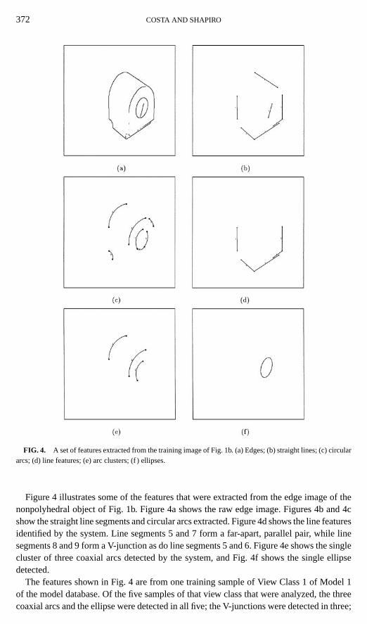
FIG. 4. A set of features extracted from the training image of Fig. 1b. (a) Edges; (b) straight lines; (c) circulararcs; (d) line features; (e) arc clusters; (f ) ellipses.
Figure 4 illustrates some of the features that were extracted from the edge image of thenonpolyhedral object of Fig. 1b. Figure 4a shows the raw edge image. Figures 4b and 4cshow the straight line segments and circular arcs extracted. Figure 4d shows the line featuresidentified by the system. Line segments 5 and 7 form a far-apart, parallel pair, while linesegments 8 and 9 form a V-junction as do line segments 5 and 6. Figure 4e shows the singlecluster of three coaxial arcs detected by the system, and Fig. 4f shows the single ellipsedetected.
The features shown in Fig. 4 are from one training sample of View Class 1 of Model 1of the model database. Of the five samples of that view class that were analyzed, the threecoaxial arcs and the ellipse were detected in all five; the V-junctions were detected in three;
3D OBJECT RECOGNITION AND RELATIONAL INDEXING 373
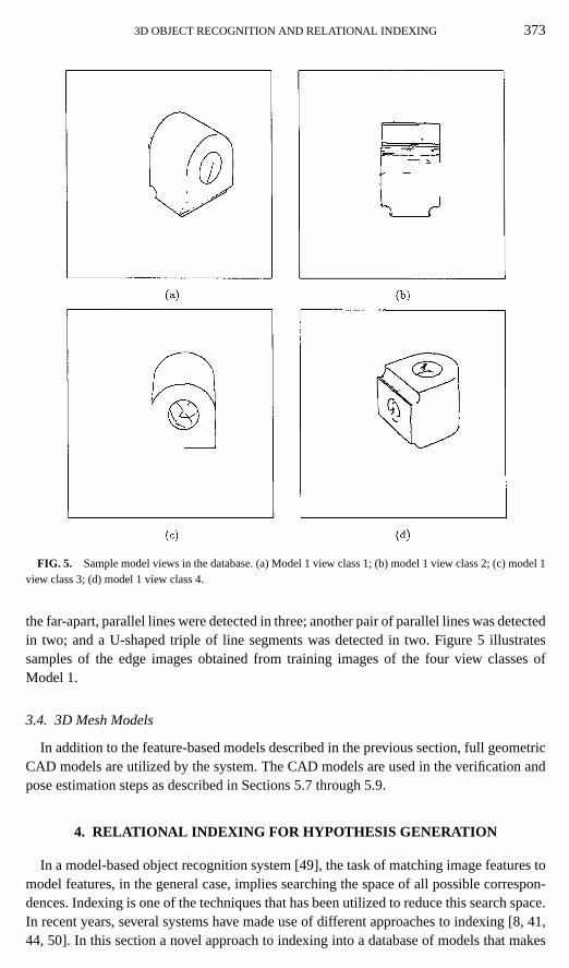
FIG. 5. Sample model views in the database. (a) Model 1 view class 1; (b) model 1 view class 2; (c) model 1view class 3; (d) model 1 view class 4.
the far-apart, parallel lines were detected in three; another pair of parallel lines was detectedin two; and a U-shaped triple of line segments was detected in two. Figure 5 illustratessamples of the edge images obtained from training images of the four view classes ofModel 1.
3.4. 3D Mesh Models
In addition to the feature-based models described in the previous section, full geometricCAD models are utilized by the system. The CAD models are used in the verification andpose estimation steps as described in Sections 5.7 through 5.9.
4. RELATIONAL INDEXING FOR HYPOTHESIS GENERATION
In a model-based object recognition system [49], the task of matching image features tomodel features, in the general case, implies searching the space of all possible correspon-dences. Indexing is one of the techniques that has been utilized to reduce this search space.In recent years, several systems have made use of different approaches to indexing [8, 41,44, 50]. In this section a novel approach to indexing into a database of models that makes
374 COSTA AND SHAPIRO
use of features and the relationships among them is described. This new technique is calledrelational indexing.
In relational indexing each view-class model in the database is described by a relationalgraph of all its features, but small relational subgraphs of the image features are utilized toindex into the database and retrieve appropriate model hypotheses. In this section the useof this new technique for hypothesis generation is demonstrated.
4.1. Relational Indexing Notation
An attributed relational description Dis a labeled graphD = (N, E) whereN is a setof attributed nodes andE is a set of labeled edges. For each attributed noden∈ N, let A(n)denote the attribute vector associated with noden. Each labeled edgee∈ E will be denotedase= (ni , nj , Li, j ), whereni andnj are nodes ofN, andLi, j is the label associated withthe edge between them.Li, j is usually a scalar, but it can also be a vector.
A relational descriptionD = (N, E) can be broken down into subgraphs, each havinga small number of nodes. Subgraphs of two nodes, called2-graphs, are considered. In theworst case, a complete graph ofk nodes has
(k2
)2-graphs, each consisting of a pair of
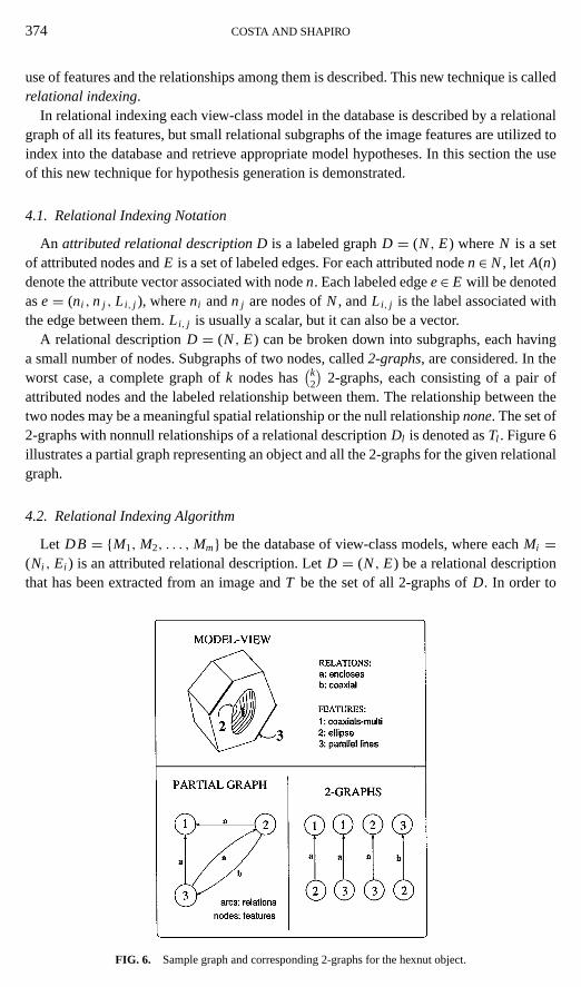
attributed nodes and the labeled relationship between them. The relationship between thetwo nodes may be a meaningful spatial relationship or the null relationshipnone. The set of2-graphs with nonnull relationships of a relational descriptionDl is denoted asTl . Figure 6illustrates a partial graph representing an object and all the 2-graphs for the given relationalgraph.
4.2. Relational Indexing Algorithm
Let DB = {M1,M2, . . . ,Mm} be the database of view-class models, where eachMi =(Ni , Ei ) is an attributed relational description. LetD = (N, E) be a relational descriptionthat has been extracted from an image andT be the set of all 2-graphs ofD. In order to
FIG. 6. Sample graph and corresponding 2-graphs for the hexnut object.
3D OBJECT RECOGNITION AND RELATIONAL INDEXING 375
find the closest models toD two steps are performed: an offline preprocessing step that setsup the indexing mechanism and an online hypotheses generation step. The offline step isas follows. LetT Mi be the set of 2-graphs ofMi . Each elementGMi
l in this set is encodedto produce an indexI Mi
l , which is used to access a lookup table. The bin corresponding toan encoded 2-graphGl stores information about which models gave rise to that particularindex. Whenever a particular 2-graphGMi
l of modelMi produces an index that accesses abin B, modelMi is added to the list of models inB. This encoding and storing of informationin the lookup table is done offline and for all models in the databaseDB.
In the online step the relational indexing procedure keeps an accumulatorAi for eachmodel Mi in the database; all the accumulators are initialized to zero. Each 2-graphGl
in T is encoded to produce an indexIl . The procedure then uses that index to retrievefrom the precomputed lookup table all modelsMi that contain a 2-graph that is identicalto Gl . Identical means that the two nodes have the same attributes and the edge has thesame label. For each 2-graphGl of T , the accumulatorAi of every retrieved modelMi isincremented by one. After the entire voting process, the models whose accumulators havethe highest votes are candidates for further consideration. Since the procedure potentiallygoes through all (k2) 2-graphs ofT and for each one can retrieve a maximum ofm models,the worst-case complexity isO(m( k
2)). However, the work performed on each model is verysmall, merely incrementing its accumulator by one. This is very different from methodsthat perform full relational matching on each model of the database. Furthermore, in realimaging applications, many of the 2-graphs have the null relationship and are not includedin the voting process. The relational indexing algorithm is given below.
RELATIONAL INDEXING ALGORITHM.
Preprocessing (offline) Phase
1. For each modelMi in the databaseDB do:• Encode each 2-graphGMi
l to produce an index.• StoreMi and associated information in the selected bin of the lookup table.
Matching (online) Phase
1. Construct a relational descriptionD for the scene.2. For each 2-graphGl of D do:• Encode it, produce an index, and access the lookup table.• Cast a vote for eachMi associated with the selected bin.
3. SelectMi ’s with enough votes as possible hypotheses.
Since some models share features and relations, it is expected that some of the hypothesesproduced will be incorrect. This indicates that a subsequent verification phase is essentialfor the method to be successful. It is important to mention that the information storedin the lookup table is actually more than just the identity of the model that gave rise to aparticular 2-graph index. It also contains information about which specific features (and theirattributes) are part of the 2-graph. This information is essential for hypothesis verificationand eventual pose estimation.
4.3. Encoding, Indexing, and Voting Schemes
In the scope of this work, only subgraphs of size two nodes were used. This meansthat each index, in the general case, is made up of a combination of two features and two
376 COSTA AND SHAPIRO
FIG. 7. Lookup table and indexing scheme.
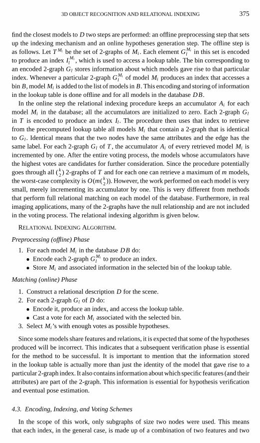
relations, indicating the two-way relationship between the features. In the implementation,each feature type and each relation are represented by distinct labels (integers). Therefore,each subgraph index is uniquely represented by a 4-tuple of integers (f1, f2, r1, r2), whichis used to access a lookup table, as shown in Figure 7. Each entry of the lookup table holdsa linked list of all model-views that gave rise to the particular 2-graph corresponding to thetable indices.
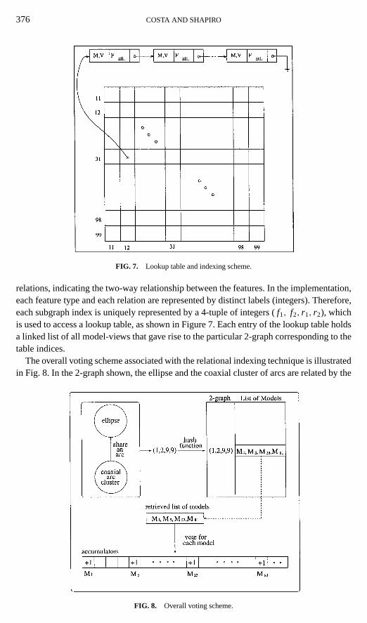
The overall voting scheme associated with the relational indexing technique is illustratedin Fig. 8. In the 2-graph shown, the ellipse and the coaxial cluster of arcs are related by the
FIG. 8. Overall voting scheme.
3D OBJECT RECOGNITION AND RELATIONAL INDEXING 377
two-way relationshare an arc.The ellipse is represented by the label “1” while the coaxialarc cluster is represented by label “2”. The relationshare an arcis represented by label“9”. Therefore, the particular 2-graph illustrated is uniquely represented by the 4-tuple (1,2, 9, 9). This gives rise to the indices used to access the lookup table: (x = 12, y = 99).The indexed bin contains a list of all models in the database which contain the subgraphused to generate the indices. In the example shown, modelsM1, M5, M23, and M81 areretrieved. The accumulators of these models are incremented by one, meaning that eachmodel receives one vote from the specific 2-graph used.
4.4. Matching with Relational Indexing: An Example
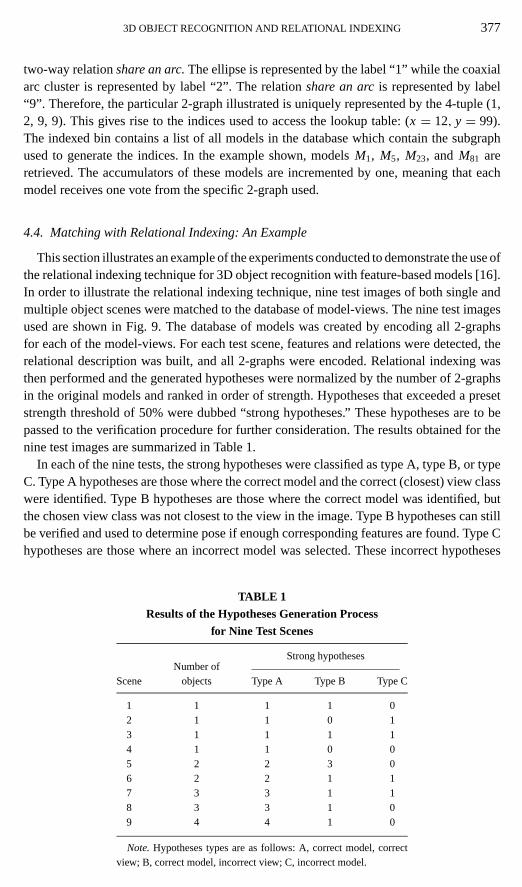
This section illustrates an example of the experiments conducted to demonstrate the use ofthe relational indexing technique for 3D object recognition with feature-based models [16].In order to illustrate the relational indexing technique, nine test images of both single andmultiple object scenes were matched to the database of model-views. The nine test imagesused are shown in Fig. 9. The database of models was created by encoding all 2-graphsfor each of the model-views. For each test scene, features and relations were detected, therelational description was built, and all 2-graphs were encoded. Relational indexing wasthen performed and the generated hypotheses were normalized by the number of 2-graphsin the original models and ranked in order of strength. Hypotheses that exceeded a presetstrength threshold of 50% were dubbed “strong hypotheses.” These hypotheses are to bepassed to the verification procedure for further consideration. The results obtained for thenine test images are summarized in Table 1.
In each of the nine tests, the strong hypotheses were classified as type A, type B, or typeC. Type A hypotheses are those where the correct model and the correct (closest) view classwere identified. Type B hypotheses are those where the correct model was identified, butthe chosen view class was not closest to the view in the image. Type B hypotheses can stillbe verified and used to determine pose if enough corresponding features are found. Type Chypotheses are those where an incorrect model was selected. These incorrect hypotheses
TABLE 1
Results of the Hypotheses Generation Process
for Nine Test Scenes
Strong hypothesesNumber of
Scene objects Type A Type B Type C
1 1 1 1 02 1 1 0 13 1 1 1 14 1 1 0 05 2 2 3 06 2 2 1 17 3 3 1 18 3 3 1 09 4 4 1 0
Note.Hypotheses types are as follows: A, correct model, correctview; B, correct model, incorrect view; C, incorrect model.

378 COSTA AND SHAPIRO
FIG. 9. The nine test scenes used. The labels left and right indicate the direction of the light source. (a) Image 1(left); (b) image 2 (right); (c) image 3 (left); (d) image 4 (left); (e) image 5 (left); (f) image 6 (right); (g) image 7 (left);(h) image 8 (right); (i) image 9 (right).
should be ruled out in the verification step. The results of the nine tests are as follows: allthe objects in the scenes have been correctly recognized (18 type A hypotheses); there werenine type B hypotheses and four type C hypotheses.
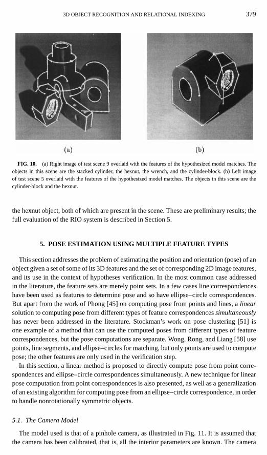
Figure 10a shows the results for test scene 9, which contains four objects: the stackedcylinder, the hexnut, the wrench, and the cylinder-block. The system produced five stronghypotheses; four were correct and are overlaid on the image. These hypothesized modelswere taken through pose computation (affine correspondence of model features and scenefeatures) without verification. The fifth strong hypothesis (not shown) matched the objecthexnut to an incorrect view of the correct object model. The subgraph indices shown inFig. 6 were among those that were used in the matching process.
Figure 10b illustrates the correct (type A) hypotheses generated for test scene 5. Of thethree type B hypotheses generated, one was for the cylinder-block object and two were for
3D OBJECT RECOGNITION AND RELATIONAL INDEXING 379
FIG. 10. (a) Right image of test scene 9 overlaid with the features of the hypothesized model matches. Theobjects in this scene are the stacked cylinder, the hexnut, the wrench, and the cylinder-block. (b) Left imageof test scene 5 overlaid with the features of the hypothesized model matches. The objects in this scene are thecylinder-block and the hexnut.
the hexnut object, both of which are present in the scene. These are preliminary results; thefull evaluation of the RIO system is described in Section 5.
5. POSE ESTIMATION USING MULTIPLE FEATURE TYPES
This section addresses the problem of estimating the position and orientation (pose) of anobject given a set of some of its 3D features and the set of corresponding 2D image features,and its use in the context of hypotheses verification. In the most common case addressedin the literature, the feature sets are merely point sets. In a few cases line correspondenceshave been used as features to determine pose and so have ellipse–circle correspondences.But apart from the work of Phong [45] on computing pose from points and lines, alinearsolution to computing pose from different types of feature correspondencessimultaneouslyhas never been addressed in the literature. Stockman’s work on pose clustering [51] isone example of a method that can use the computed poses from different types of featurecorrespondences, but the pose computations are separate. Wong, Rong, and Liang [58] usepoints, line segments, and ellipse–circles for matching, but only points are used to computepose; the other features are only used in the verification step.
In this section, a linear method is proposed to directly compute pose from point corre-spondences and ellipse–circle correspondences simultaneously. A new technique for linearpose computation from point correspondences is also presented, as well as a generalizationof an existing algorithm for computing pose from an ellipse–circle correspondence, in orderto handle nonrotationally symmetric objects.
5.1. The Camera Model
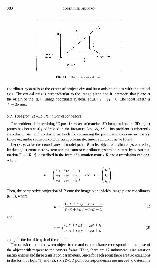
The model used is that of a pinhole camera, as illustrated in Fig. 11. It is assumed thatthe camera has been calibrated, that is, all the interior parameters are known. The camera
380 COSTA AND SHAPIRO
FIG. 11. The camera model used.
coordinate system is at the center of projectivity and itsz-axis coincides with the opticalaxis. The optical axis is perpendicular to the image plane and it intersects that plane atthe origin of the (u, v) image coordinate system. Thus,u0 = v0 = 0. The focal length isf = 25 mm.
5.2. Pose from 2D–3D Point Correspondences
The problem of determining 3D pose from sets of matched 2D image points and 3D objectpoints has been vastly addressed in the literature [28, 55, 32]. This problem is inherentlya nonlinear one, and nonlinear methods for estimating the pose parameters are necessary.However, under some conditions, an approximate, linear solution can be found.
Let (x, y, z) be the coordinates of model pointP in its object coordinate system. Also,let the object coordinate system and the camera coordinate system be related by a transfor-mationT = {R, t}, described in the form of a rotation matrixR and a translation vectort ,where
R= r11 r12 r13
r21 r22 r23
r31 r32 r33
and t =
txty
tz
.Then, the perspective projection ofP onto the image plane yields image plane coordinates(u, v), where
u = fr11x + r12y+ r13z+ txr31x + r32y+ r33z+ tz
(1)
and
v = fr21x + r22y+ r23z+ ty
r31x + r32y+ r33z+ tz, (2)
and f is the focal length of the camera.The transformation between object frame and camera frame corresponds to the pose of
the object with respect to the camera frame. Thus, there are 12 unknowns: nine rotationmatrix entries and three translation parameters. Since for each point there are two equationsin the form of Eqs. (1) and (2), six 2D–3D point correspondences are needed to determine
3D OBJECT RECOGNITION AND RELATIONAL INDEXING 381
all the pose parameters. The resulting system of equations is of the form
Bw = 0, (3)
where
B =
f x1 f y1 f z1 0 0 0 −u1x1 −u1y1 −u1z1 f 0 −u1
0 0 0 f x1 f y1 f z1 −v1x1 −v1y1 −v1z1 0 f −v1
f x2 f y2 f z2 0 0 0 −u2x2 −u2y2 −u2z2 f 0 −u2
0 0 0 f x2 f y2 f z2 −v2x2 −v2y2 −v2z2 0 f −v2...
......
......
......
......
......
...
f x6 f y6 f z6 0 0 0 −u6x6 −u6y6 −u6z6 f 0 −u6
0 0 0 f x6 f y6 f z6 −v6x6 −v6y6 −v6z6 0 f −v6
(4)
and
w = (r11 r12 r13 r21 r22 r23 r31 r32 r33 tx ty tz)T . (5)
However, if one is interested in finding the true pose parameters, and not simply atransformation that aligns the projected model points well to the image points, conditionsneed to be imposed on the elements ofR such that it satisfies all the criteria a true 3Drotation matrix must satisfy. In particular, a rotation matrix needs to be orthonormal: its rowvectors must have magnitude equal to one, and they must be orthogonal to each other. Thiscan be written as:
‖R1‖ = r 211+ r 2
12+ r 213 = 1
‖R2‖ = r 221+ r 2
22+ r 223 = 1 (6)
‖R3‖ = r 231+ r 2
32+ r 233 = 1
and
R1 ◦ R2 = 0
R1 ◦ R3 = 0 (7)
R2 ◦ R3 = 0.
In fact, theoretically, there is an infinite number of transformations of the formT = {R, t}that will produce coordinates (u, v) for a givenP that yield an acceptable “alignment,” butthere is only oneT = {R, t}, for which R and t correspond to the true 3D position andorientation of the object relative to the camera frame.
It can be seen that the conditions imposed onR turn the problem into a nonlinear one.If the conditions on the magnitudes of the row vectors ofR are imposed one at a time,and computed independently, a linear constrained optimization technique similar to the oneused by Faugeras [25] can be used to compute the constrained row vector ofR.
382 COSTA AND SHAPIRO
5.3. Linear Constrained Optimization
Given the system of equations (3), the problem at hand is to find the solution vectorw thatminimizes‖Bw‖ subject to the constraint‖w′‖2 = 1, wherew′ is a subset of the elementsof w. If the constraint is to be imposed on the first row vector ofR, then
w′ = r11
r12
r13
.To solve the above problem, it is necessary to rewrite the original system of equationsBw = 0 in the following form
Cw′ + Dw′′ = 0,
wherew′′ is a vector with the remaining elements ofw. Using the example above, i.e., ifthe constraint is imposed on the first row ofR,
w′′ = (r21 r22 r23 r31 r32 r33 tx ty tz)T .
The original problem can be stated as: minimize the objective functionO = Cw′ + Dw′′,that is
minw′,w′′‖Cw′ + Dw′′‖2, (8)
subject to the constraint‖w′‖2 = 1. Using a Lagrange multiplier technique, the above isequivalent to
minw′,w′′
[‖Cw′ + Dw′′‖2+ λ(1− ‖w′‖2)]. (9)
The minimization problem above can be solved by taking partial derivatives of the objectivefunction with respect tow′ andw′′ and equating them to zero:
∂O
∂w′= 2CT (Cw′ + Dw′′)− 2λw′ = 0 (10)
∂O
∂w′′= 2DT (Cw′ + Dw′′) = 0. (11)
Equation (11) is equivalent to
w′′ = −(DT D)−1DTCw′. (12)
Substituting Eq. (12) into Eq. (10) yields
λw′ = [CTC − CT D(DT D)−1DTC]w′. (13)
It can be seen thatλ is an eigenvector of the matrix
M = CTC − CT D(DT D)−1DTC. (14)
3D OBJECT RECOGNITION AND RELATIONAL INDEXING 383
Therefore, the solution sought forw′ corresponds to the smallest eigenvector associatedwith matrixM . The correspondingw′′ can be directly computed from Eq. (12). It is importantto notice that since the magnitude constraint was imposed only on one of the rows ofR, theresults obtained forw′′ are not reliable and therefore should not be used. However, solutionvectorw′′ provides an important piece of information regarding the sign of the row vectoron which the constraint was imposed. The constraint imposed was‖w′‖2 = 1, but the signof w′ is not restricted by this constraint. Therefore, it is necessary to check whether or notthe resultingw′ yields a solution that is physically possible. In particular, the translationtzmust be positive in order for the object to be located in front of the camera as opposed tobehind it. If the element of vectorw′′ that corresponds totz is negative, it means that themagnitude of the computedw′ is correct, but its sign is not, and it must be changed. Thus,the final expression for the computedw′ is
w′ = sign(w′′9)w′.
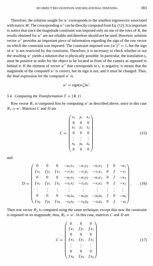
5.4. Computing the Transformation T= {R, t}Row vectorR1 is computed first by computingw′ as described above, since in this case
R1 = w′. MatricesC andD are
C =
x1 y1 z1
0 0 0x2 y2 z2
0 0 0...
......
x6 y6 z6
0 0 0
(15)
and
D =
0 0 0 −u1x1 −u1y1 −u1z1 f 0 −u1
f x1 f y1 f z1 −v1x1 −v1y1 −v1z1 0 f −v1
0 0 0 −u2x2 −u2y2 −u2z2 0 f −u2
f x2 f y2 f z2 −v2x2 −v2y2 −v2z2 0 f −v2...
......
......
......
......
0 0 0 −u6x6 −u6y6 −u6z6 f 0 −u6
f x6 f y6 f z6 −v6x6 −v6y6 −v6z6 0 f −v6
. (16)
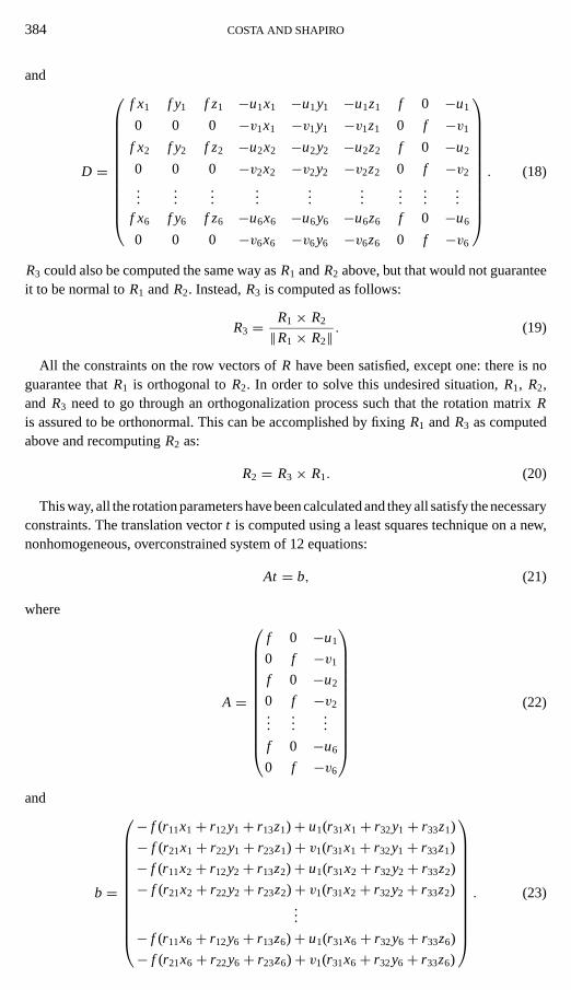
Then row vectorR2 is computed using the same technique, except that now the constraintis imposed on its magnitude; thus,R2 = w′. In this case, matricesC andD are
C =
0 0 0f x1 f y1 f z1
0 0 0f x2 f y2 f z2...
......
0 0 0f x6 f y6 f z6
(17)
384 COSTA AND SHAPIRO
and
D =
f x1 f y1 f z1 −u1x1 −u1y1 −u1z1 f 0 −u1
0 0 0 −v1x1 −v1y1 −v1z1 0 f −v1
f x2 f y2 f z2 −u2x2 −u2y2 −u2z2 f 0 −u2
0 0 0 −v2x2 −v2y2 −v2z2 0 f −v2
......
......
......
......
...f x6 f y6 f z6 −u6x6 −u6y6 −u6z6 f 0 −u6
0 0 0 −v6x6 −v6y6 −v6z6 0 f −v6
. (18)
R3 could also be computed the same way asR1 andR2 above, but that would not guaranteeit to be normal toR1 andR2. Instead,R3 is computed as follows:
R3 = R1× R2
‖R1× R2‖ . (19)
All the constraints on the row vectors ofR have been satisfied, except one: there is noguarantee thatR1 is orthogonal toR2. In order to solve this undesired situation,R1, R2,and R3 need to go through an orthogonalization process such that the rotation matrixRis assured to be orthonormal. This can be accomplished by fixingR1 andR3 as computedabove and recomputingR2 as:
R2 = R3× R1. (20)
This way, all the rotation parameters have been calculated and they all satisfy the necessaryconstraints. The translation vectort is computed using a least squares technique on a new,nonhomogeneous, overconstrained system of 12 equations:
At = b, (21)
where
A =
f 0 −u1
0 f −v1
f 0 −u2
0 f −v2...
......
f 0 −u6
0 f −v6
(22)
and
b =
− f (r11x1+ r12y1+ r13z1)+ u1(r31x1+ r32y1+ r33z1)
− f (r21x1+ r22y1+ r23z1)+ v1(r31x1+ r32y1+ r33z1)
− f (r11x2+ r12y2+ r13z2)+ u1(r31x2+ r32y2+ r33z2)
− f (r21x2+ r22y2+ r23z2)+ v1(r31x2+ r32y2+ r33z2)...
− f (r11x6+ r12y6+ r13z6)+ u1(r31x6+ r32y6+ r33z6)
− f (r21x6+ r22y6+ r23z6)+ v1(r31x6+ r32y6+ r33z6)
. (23)

3D OBJECT RECOGNITION AND RELATIONAL INDEXING 385
5.5. Pose from Ellipse-to-Circle Correspondence
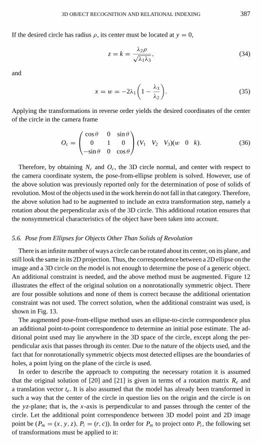
In order to find the 3D position and orientation of a circle from its projection onto theimage plane (an ellipse in the general case) the solution described in [20] and [21] is utilized.The solution consists of a series of 3D transformations to the circle and it is carried out intwo stages: first the orientation of the 3D plane on which the circle lies is determined; andthen the center of the circle is computed.
An ellipse in the image plane is of the following form
a1x2+ a2xy+ a3y2+ a4x + a5y+ a6 = 0. (24)
Since one of the assumptions about the geometry is that the origin is at the principal point,this ellipse defines a cone in 3D,
a1x2+ a2xy+ a3y2+ a4
fxz+ a5
fyz+ a6
fz2 = 0, (25)
where f is the focal length of the camera. Equation (25) above can be written in the formXTC X = 0, where
C =
a1
a22
a42 f
a22 a3
a52 f
a42 f
a52 f
a6f 2
(26)
and
X = (x y z)T . (27)
In order to find the orientation of the plane on which the circle lies, it is necessary to firstreduce the cone equation to
x2
b1+ y2
b2+ z2
f 2= 0.
This is accomplished by a 3D rotation to the eigenvector frame such thatC becomes adiagonal matrix of the form
C′ =
λ1 0 0
0 λ2 0
0 0 λ3
, (28)
whereλ1, λ2, andλ3 are the eigenvalues ofC in ascending order. The rotation matrix thataccomplishes the above is given by
Rλ = (V1 V2 V3), (29)
whereV1, V2, andV3 are the eigenvectors ofC. Then, another rotation about the newy-axisis performed such that the intersection of the cone with the planez= k is a circle. Thus,
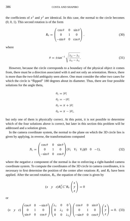
386 COSTA AND SHAPIRO
the coefficients ofx2 and y2 are identical. In this case, the normal to the circle becomes(0, 0, 1). This second rotation is of the form
Rθ =
cosθ 0 sinθ
0 1 0
−sinθ 0 cosθ
, (30)
where
θ = ±tan−1
√λ2− λ1
λ3− λ1. (31)
However, because the circle corresponds to a boundary of the physical object it comesfrom, there must be a direction associated with it and not only an orientation. Hence, thereis more than the two-fold ambiguity seen above. One must consider the other two cases forwhich the circle is “flipped” 180 degrees about its diameter. Thus, there are four possiblesolutions for the angle theta,
θ1 = |θ |θ2 = −|θ |θ3 = π + |θ |θ4 = π − |θ |,
but only one of them is physically correct. At this point, it is not possible to determinewhich of the four solutions above is correct, but later in this section this problem will beaddressed and a solution given.
In the camera coordinate system, the normal to the plane on which the 3D circle lies isgiven by applying, in reverse, the transformations computed
Nc =
cosθ 0 sinθ
0 1 0
−sinθ 0 cosθ
(V1 V2 V3)(0 0 −1), (32)
where the negativez component of the normal is due to enforcing a right-handed cameracoordinate system. To compute the coordinates of the 3D circle in camera coordinates, it isnecessary to first determine the position of the center after rotationsRλ andRθ have beenapplied. After the second rotation,Rθ , the equation of the cone is given by
(x y z)RTθ C′Rθ
xyz
= 0
or
(x y z)
cosθ 0 −sinθ
0 1 0
sinθ 0 cosθ
λ1 0 0
0 λ2 0
0 0 λ3
cosθ 0 sinθ
0 1 0
−sinθ 0 cosθ
x
yz
= 0. (33)
3D OBJECT RECOGNITION AND RELATIONAL INDEXING 387
If the desired circle has radiusρ, its center must be located aty = 0,
z= k = λ2ρ√λ1λ3
, (34)
and
x = w = −2λ1
(1− λ3
λ2
). (35)
Applying the transformations in reverse order yields the desired coordinates of the centerof the circle in the camera frame
Oc = cosθ 0 sinθ
0 1 0−sinθ 0 cosθ
(V1 V2 V3)(w 0 k). (36)
Therefore, by obtainingNc and Oc, the 3D circle normal, and center with respect tothe camera coordinate system, the pose-from-ellipse problem is solved. However, use ofthe above solution was previously reported only for the determination of pose of solids ofrevolution. Most of the objects used in the work herein do not fall in that category. Therefore,the above solution had to be augmented to include an extra transformation step, namely arotation about the perpendicular axis of the 3D circle. This additional rotation ensures thatthe nonsymmetrical characteristics of the object have been taken into account.
5.6. Pose from Ellipses for Objects Other Than Solids of Revolution
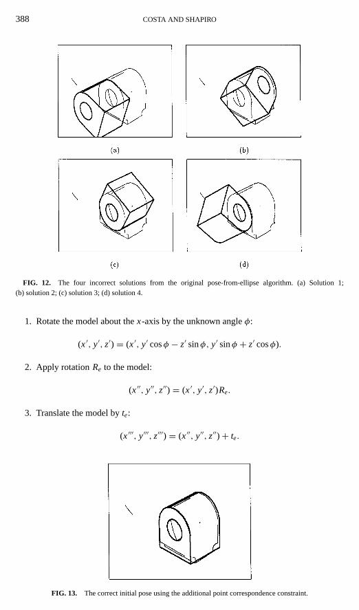
There is an infinite number of ways a circle can be rotated about its center, on its plane, andstill look the same in its 2D projection. Thus, the correspondence between a 2D ellipse on theimage and a 3D circle on the model is not enough to determine the pose of a generic object.An additional constraint is needed, and the above method must be augmented. Figure 12illustrates the effect of the original solution on a nonrotationally symmetric object. Thereare four possible solutions and none of them is correct because the additional orientationconstraint was not used. The correct solution, when the additional constraint was used, isshown in Fig. 13.
The augmented pose-from-ellipse method uses an ellipse-to-circle correspondence plusan additional point-to-point correspondence to determine an initial pose estimate. The ad-ditional point used may lie anywhere in the 3D space of the circle, except along the per-pendicular axis that passes through its center. Due to the nature of the objects used, and thefact that for nonrotationally symmetric objects most detected ellipses are the boundaries ofholes, a point lying on the plane of the circle is used.
In order to describe the approach to computing the necessary rotation it is assumedthat the original solution of [20] and [21] is given in terms of a rotation matrixRe anda translation vectorte. It is also assumed that the model has already been transformed insuch a way that the center of the circle in question lies on the origin and the circle is onthe yz-plane; that is, thex-axis is perpendicular to and passes through the center of thecircle. Let the additional point correspondence between 3D model point and 2D imagepoint be (Pm = (x, y, z), Pi = (r, c)). In order forPm to project ontoPi , the following setof transformations must be applied to it:
388 COSTA AND SHAPIRO
FIG. 12. The four incorrect solutions from the original pose-from-ellipse algorithm. (a) Solution 1;(b) solution 2; (c) solution 3; (d) solution 4.
1. Rotate the model about thex-axis by the unknown angleφ:
(x′, y′, z′) = (x′, y′ cosφ − z′ sinφ, y′ sinφ + z′ cosφ).
2. Apply rotationRe to the model:
(x′′, y′′, z′′) = (x′, y′, z′)Re.
3. Translate the model byte:
(x′′′, y′′′, z′′′) = (x′′, y′′, z′′)+ te.
FIG. 13. The correct initial pose using the additional point correspondence constraint.
3D OBJECT RECOGNITION AND RELATIONAL INDEXING 389
4. Project the translated model onto the image plane:
(r, c) =(
fx′′′
z′′′, f
y′′′
z′′′
), where f is the focal length of the camera.
In order to determine the unknown rotation angleφ, notice that:
r
x′′′= c
y′′′.
The above leads to a trigonometric equation onφ of the formA sinφ + B cosφ + C = 0,which yields the following two solutions,
φ = 2 arctan(−A+
√(A2+ B2− c2))
−B+ C(37)
and
φ = 2 arctan(−A−
√(A2+ B2− c2))
−B+ C, (38)
where
A = y(re31 − kre32
)+ z(kre22 − re21
),
B = y(re21 − kre22
)+ z(re31 − kre32
), (39)
C = x(re11 − kre12
)+ tex − ktey,
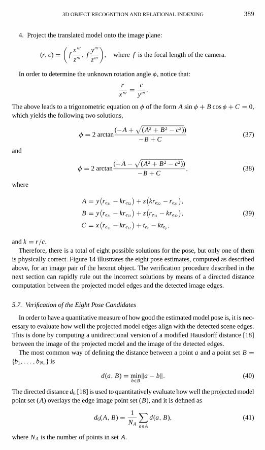
andk = r/c.Therefore, there is a total of eight possible solutions for the pose, but only one of them
is physically correct. Figure 14 illustrates the eight pose estimates, computed as describedabove, for an image pair of the hexnut object. The verification procedure described in thenext section can rapidly rule out the incorrect solutions by means of a directed distancecomputation between the projected model edges and the detected image edges.
5.7. Verification of the Eight Pose Candidates
In order to have a quantitative measure of how good the estimated model pose is, it is nec-essary to evaluate how well the projected model edges align with the detected scene edges.This is done by computing a unidirectional version of a modified Hausdorff distance [18]between the image of the projected model and the image of the detected edges.
The most common way of defining the distance between a pointa and a point setB ={b1, . . . ,bNB} is
d(a, B) = minb∈B‖a− b‖. (40)
The directed distanced6 [18] is used to quantitatively evaluate how well the projected modelpoint set (A) overlays the edge image point set (B), and it is defined as
d6(A, B) = 1
NA
∑a∈A
d(a, B), (41)
whereNA is the number of points in setA.
390 COSTA AND SHAPIRO
FIG. 14. The eight solutions from the constrained pose-from-ellipse algorithm. (a) Solution 1; (b) solution 2;(c) solution 3; (d) solution 4; (e) solution 5; (f ) solution 6; (g) solution 7; (h) solution 8.
For the specific verification task required in this work, the directed distance measure isutilized because it is necessary to account for occlusion as well as extra points in setB,since, in the general case, there are multiple objects in the image. The above measure hasbeen shown to rule out the pose hypotheses that are obviously incorrect. Results to thiseffect are given in Section 6.
5.8. Generalized Pose Computation from Ellipses and Points
In the two previous sections two different methods for computing pose from differentfeatures were described. However, it is desirable to be able to compute pose from morethan one type of featuresimultaneously. The reason is quite obvious: it will provide a moreaccurate solution. This section is devoted to formulating a method of computing pose from2D–3D point correspondences and ellipse–circle correspondences, simultaneously.
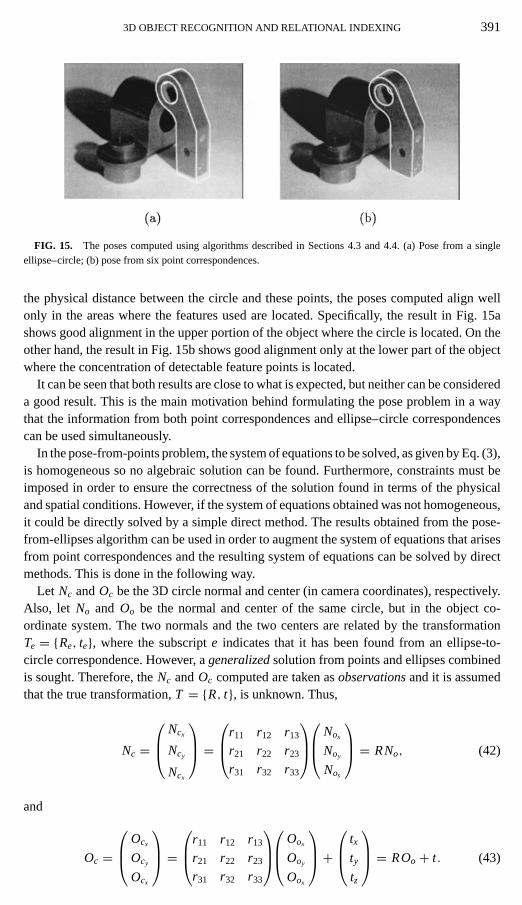
To exemplify the issue of accuracy addressed in the paragraph above, the results of thepose estimation from points alone and from one ellipse are shown in Figs. 15a and 15b,respectively. Notice that due to the localized concentration of detectable feature points and
3D OBJECT RECOGNITION AND RELATIONAL INDEXING 391
FIG. 15. The poses computed using algorithms described in Sections 4.3 and 4.4. (a) Pose from a singleellipse–circle; (b) pose from six point correspondences.
the physical distance between the circle and these points, the poses computed align wellonly in the areas where the features used are located. Specifically, the result in Fig. 15ashows good alignment in the upper portion of the object where the circle is located. On theother hand, the result in Fig. 15b shows good alignment only at the lower part of the objectwhere the concentration of detectable feature points is located.
It can be seen that both results are close to what is expected, but neither can be considereda good result. This is the main motivation behind formulating the pose problem in a waythat the information from both point correspondences and ellipse–circle correspondencescan be used simultaneously.
In the pose-from-points problem, the system of equations to be solved, as given by Eq. (3),is homogeneous so no algebraic solution can be found. Furthermore, constraints must beimposed in order to ensure the correctness of the solution found in terms of the physicaland spatial conditions. However, if the system of equations obtained was not homogeneous,it could be directly solved by a simple direct method. The results obtained from the pose-from-ellipses algorithm can be used in order to augment the system of equations that arisesfrom point correspondences and the resulting system of equations can be solved by directmethods. This is done in the following way.
Let Nc andOc be the 3D circle normal and center (in camera coordinates), respectively.Also, let No and Oo be the normal and center of the same circle, but in the object co-ordinate system. The two normals and the two centers are related by the transformationTe = {Re, te}, where the subscripte indicates that it has been found from an ellipse-to-circle correspondence. However, ageneralizedsolution from points and ellipses combinedis sought. Therefore, theNc andOc computed are taken asobservationsand it is assumedthat the true transformation,T = {R, t}, is unknown. Thus,
Nc =
Ncx
Ncy
Ncx
=r11 r12 r13
r21 r22 r23
r31 r32 r33
Nox
Noy
Nos
= RNo, (42)
and
Oc =
Ocx
Ocy
Ocx
=r11 r12 r13
r21 r22 r23
r31 r32 r33
Oox
Ooy
Oox
+ tx
ty
tz
= ROo + t. (43)
392 COSTA AND SHAPIRO
Furthermore, sinceR−1 = RT , No can be written as
No =
Nox
Noy
Noz
=r11 r21 r31
r12 r22 r32
r13 r23 r33
Ncx
Ncy
Ncz
= RT Nc. (44)
Notice that Eqs. (42) and (44), if used simultaneously, enforce the condition that the unknownrotation matrix be orthonormal. Equations (42)–(44) involve the same 12 unknowns as inthe system of equations (3). Hence, that system is augmented by those three equationsgiving rise to the following new system
B′w = k, (45)
where
B′ =
f x1 f y1 f z1 0 0 0 −u1x1 −u1y1 −u1z1 f 0 −u1
0 0 0 f x1 f y1 f z1 −v1x1 −v1y1 −v1z1 0 f −v1
f x2 f y2 f z2 0 0 0 −u2x2 −u2y2 −u2z2 f 0 −u2
0 0 0 f x2 f y2 f z2 −v2x2 −v2y2 −v2z2 0 f −v2...
......
......
......
......
......
...f x6 f y6 f z6 0 0 0 −u6x6 −u6y6 −u6z6 f 0 −u6
0 0 0 f x6 f y6 f z6 −v6x6 −v6y6 −v6z6 0 f −v6
Nox Noy Nox 0 0 0 0 0 0 0 0 0
0 0 0 Nox Noy Noz 0 0 0 0 0 0
0 0 0 0 0 0 Nox Noy Noz 0 0 0
Oox Ooy Ooz 0 0 0 0 0 0 1 0 0
0 0 0 Oox Ooy Ooz 0 0 0 0 1 0
0 0 0 0 0 0 Oox Ooy Ooz 0 0 1
Ncx 0 0 Ncy 0 0 Ncz 0 0 0 0 0
0 Ncx 0 0 Ncy 0 0 Ncz 0 0 0 0
0 0 Ncx 0 0 Ncy 0 0 Ncz 0 0 0
,
(46)
w = (r11 r12 r13 r21 r22 r23 r31 r32 r33 tx ty tz)T , (47)
and
k = (0 0 . . . 0 0 Ncx Ncy Ncz Ocx Ocy Ocz Nox Noy Noz
)T. (48)
The system above can be solved by a direct least-squares solution of the form
w = (B′T B′)−1B′Tk. (49)
It can be seen that since nine new equations have been added to the system, there is no needfor all six point correspondences in order to solve for the 12 transformation unknowns.However, matrixB′ must be full rank and, therefore, at least three points must be used.
3D OBJECT RECOGNITION AND RELATIONAL INDEXING 393
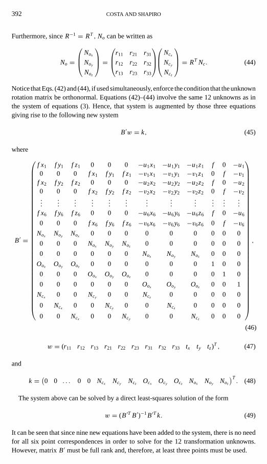
FIG. 16. The pose computed from six point correspondences and one ellipse–circle correspondence using thegeneralized methodology. Note the gap between the object and the projected model at the very top of the object.
Figure 16 illustrates the pose computed for the same image of Figs. 15a and 15b using thegeneralized pose estimation technique and making use of the same six point correspondencesand the same ellipse correspondence previously used.
Visual inspection of the results in Figs. 15a, 15b, and 16 shows the superiority of thenew technique over the other single-feature methods. The projection of the CAD modelonto the image using the transformation matrix obtained using the new technique yieldsa better alignment than those projections obtained using only point correspondences or asingle ellipse–circle correspondence. In order to compare the results quantitatively, Table 2shows the pose transformations obtained for each linear method used. Also shown in thelast row of Table 2 is the final transformation obtained after convergence of the iterative,nonlinear Gauss–Newton method [33]. The nonlinear method requires an initial guess; theresults of the linear methods (points only, circle–ellipse only, and points and circle–ellipsetogether) have been used as such. The final results after convergence of the iterative methodare the same regardless of which initial guess was used; the difference lies in the number ofiterations it took for the method to converge to the final solution. These results are reportedin [39]. The model projection for the solution obtained using the nonlinear method is shownin Fig. 17.
TABLE 2
Pose Results from Different Methods
Method R t
Points only (−43.125−25.511 1232.036)(
0.410 −0.129 −0.9020.606 −0.700 0.376−0.681 −0.701 −0.208
)Circle only (−35.161−15.358 1195.293)
(0.302 0.302 −0.9320.692 −0.628 0.355−0.655 −0.753 −0.054
)Points and circle (−43.077−26.400 1217.855)
(0.398 −0.142 −0.9020.554 −0.667 0.336−0.700 −0.684 −0.201
)Nonlinear (−43.23−28.254 1273.07)
(0.341 −0.156 −0.9270.631 −0.693 0.349−0.697 −0.704 −0.137
)
394 COSTA AND SHAPIRO
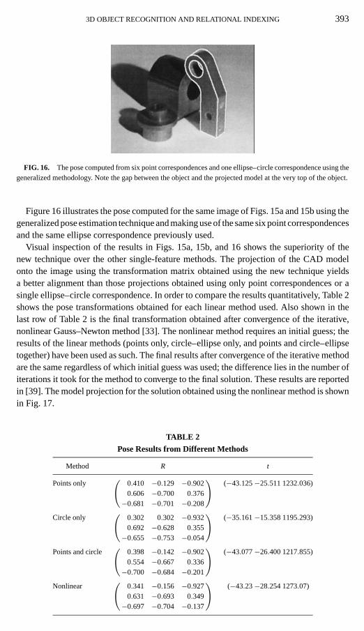
FIG. 17. The final pose obtained using the solution in Fig. 16 as the initial solution to a nonlinear least-squarespose estimation procedure. Note that the gap between the object and its features is now gone.
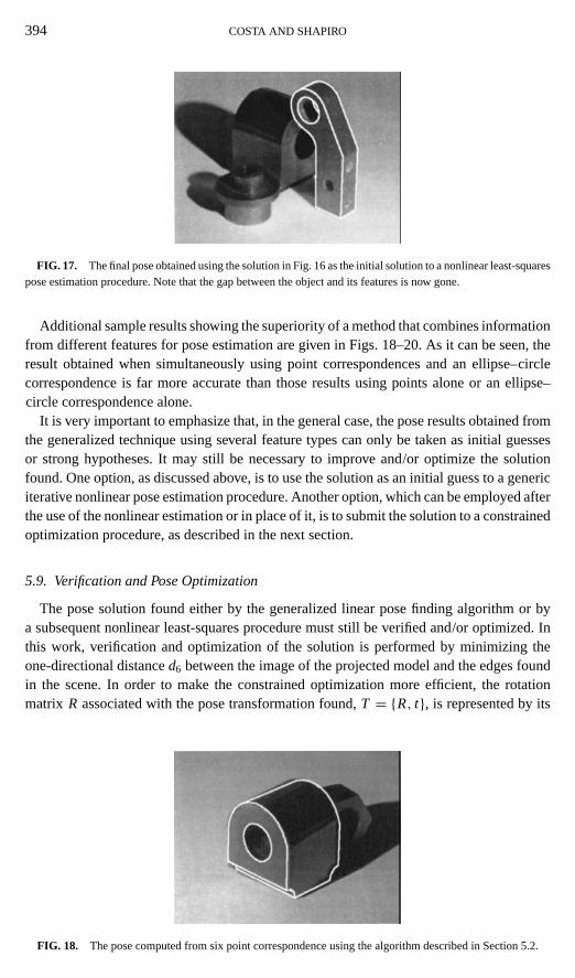
Additional sample results showing the superiority of a method that combines informationfrom different features for pose estimation are given in Figs. 18–20. As it can be seen, theresult obtained when simultaneously using point correspondences and an ellipse–circlecorrespondence is far more accurate than those results using points alone or an ellipse–circle correspondence alone.
It is very important to emphasize that, in the general case, the pose results obtained fromthe generalized technique using several feature types can only be taken as initial guessesor strong hypotheses. It may still be necessary to improve and/or optimize the solutionfound. One option, as discussed above, is to use the solution as an initial guess to a genericiterative nonlinear pose estimation procedure. Another option, which can be employed afterthe use of the nonlinear estimation or in place of it, is to submit the solution to a constrainedoptimization procedure, as described in the next section.
5.9. Verification and Pose Optimization
The pose solution found either by the generalized linear pose finding algorithm or bya subsequent nonlinear least-squares procedure must still be verified and/or optimized. Inthis work, verification and optimization of the solution is performed by minimizing theone-directional distanced6 between the image of the projected model and the edges foundin the scene. In order to make the constrained optimization more efficient, the rotationmatrix R associated with the pose transformation found,T = {R, t}, is represented by its
FIG. 18. The pose computed from six point correspondence using the algorithm described in Section 5.2.
3D OBJECT RECOGNITION AND RELATIONAL INDEXING 395
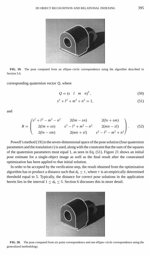
FIG. 19. The pose computed from an ellipse–circle correspondence using the algorithm described inSection 5.6.
corresponding quaternion vectorQ, where
Q = (s l m n)T , (50)
s2+ l 2+m2+ n2 = 1, (51)
and
R=
s2+ l 2−m2− n2 2(lm− sn) 2(ln + sm)
2(lm+ sn) s2− l 2+m2− n2 2(mn− sl)
2(ln − sm) 2(mn+ sl) s2− l 2−m2+ n2
. (52)
Powell’s method [19] in the seven-dimensional space of the pose solution (four quaternionparameters and the translationt) is used, along with the constraint that the sum of the squaresof the quaternion parameters must equal 1, as seen in Eq. (51). Figure 21 shows an initialpose estimate for a single-object image as well as the final result after the constrainedoptimization has been applied to that initial solution.
In order to be accepted by the verification step, the result obtained from the optimizationalgorithm has to produce a distance such thatd6 ≤ τ , whereτ is an empirically determinedthreshold equal to 5. Typically, the distance for correct pose solutions in the applicationherein lies in the interval 1≤ d6 ≤ 5. Section 6 discusses this in more detail.
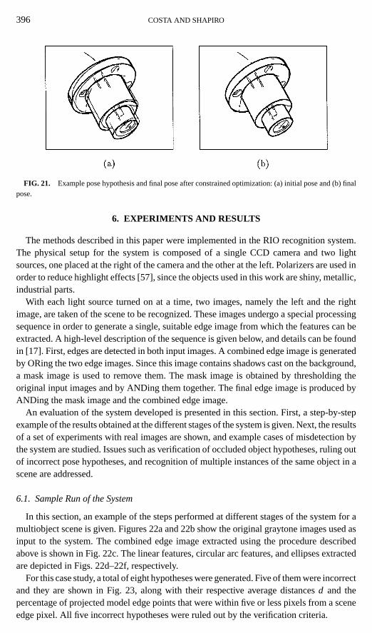
FIG. 20. The pose computed from six point correspondence and one ellipse–circle correspondence using thegeneralized methodology.
396 COSTA AND SHAPIRO
FIG. 21. Example pose hypothesis and final pose after constrained optimization: (a) initial pose and (b) finalpose.
6. EXPERIMENTS AND RESULTS
The methods described in this paper were implemented in the RIO recognition system.The physical setup for the system is composed of a single CCD camera and two lightsources, one placed at the right of the camera and the other at the left. Polarizers are used inorder to reduce highlight effects [57], since the objects used in this work are shiny, metallic,industrial parts.
With each light source turned on at a time, two images, namely the left and the rightimage, are taken of the scene to be recognized. These images undergo a special processingsequence in order to generate a single, suitable edge image from which the features can beextracted. A high-level description of the sequence is given below, and details can be foundin [17]. First, edges are detected in both input images. A combined edge image is generatedby ORing the two edge images. Since this image contains shadows cast on the background,a mask image is used to remove them. The mask image is obtained by thresholding theoriginal input images and by ANDing them together. The final edge image is produced byANDing the mask image and the combined edge image.
An evaluation of the system developed is presented in this section. First, a step-by-stepexample of the results obtained at the different stages of the system is given. Next, the resultsof a set of experiments with real images are shown, and example cases of misdetection bythe system are studied. Issues such as verification of occluded object hypotheses, ruling outof incorrect pose hypotheses, and recognition of multiple instances of the same object in ascene are addressed.
6.1. Sample Run of the System
In this section, an example of the steps performed at different stages of the system for amultiobject scene is given. Figures 22a and 22b show the original graytone images used asinput to the system. The combined edge image extracted using the procedure describedabove is shown in Fig. 22c. The linear features, circular arc features, and ellipses extractedare depicted in Figs. 22d–22f, respectively.
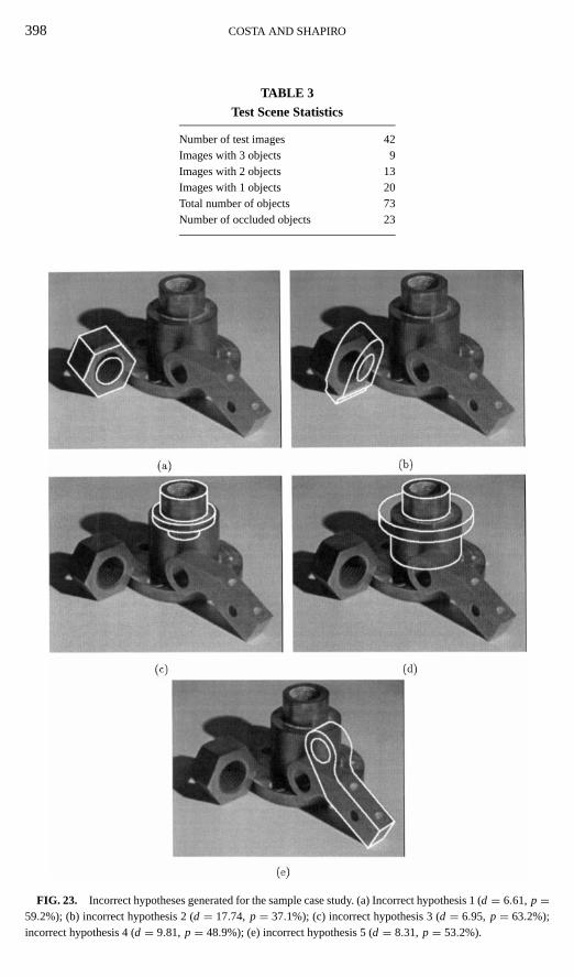
For this case study, a total of eight hypotheses were generated. Five of them were incorrectand they are shown in Fig. 23, along with their respective average distancesd and thepercentage of projected model edge points that were within five or less pixels from a sceneedge pixel. All five incorrect hypotheses were ruled out by the verification criteria.

3D OBJECT RECOGNITION AND RELATIONAL INDEXING 397
FIG. 22. Sample run of the system. (a) Original left image; (b) original right image; (c) combined edge image;(d) linear features detected; (e) circular arc features detected; (f ) ellipses detected.
The correct hypotheses generated by the system are shown in Fig. 24. All three correcthypotheses were accepted as valid by the verification criteria, since they all satisfiedd ≤ 5and p ≥ 65%.
6.2. Experiments on a Set of Real Images
Forty-two pairs of real images were used to evaluate the performance of the overallrecognition system. These images were obtained from scenes containing up to three objects,since the camera configuration we used was not able to accurately detect features in largerscenes; 9 of them contain 3 objects, 13 contain 2 objects, and 20 contain a single object.Of the total number of 73 objects in the test scenes, 23 are partially occluded by one ortwo objects. These statistics about the test images are shown in Table 3. The images were
398 COSTA AND SHAPIRO
TABLE 3
Test Scene Statistics
Number of test images 42Images with 3 objects 9Images with 2 objects 13Images with 1 objects 20Total number of objects 73Number of occluded objects 23
FIG. 23. Incorrect hypotheses generated for the sample case study. (a) Incorrect hypothesis 1 (d = 6.61, p =59.2%); (b) incorrect hypothesis 2 (d = 17.74, p = 37.1%); (c) incorrect hypothesis 3 (d = 6.95, p = 63.2%);incorrect hypothesis 4 (d = 9.81, p = 48.9%); (e) incorrect hypothesis 5 (d = 8.31, p = 53.2%).

3D OBJECT RECOGNITION AND RELATIONAL INDEXING 399
FIG. 24. Correct hypotheses generated for the sample case study (a) Correct hypothesis 1 (d = 3.30, p =83.1%); (b) correct hypothesis 2 (d = 3.84, p = 79.5%); (c) correct hypothesis 3 (d = 3.92, p = 83.5%).
matched to a database of 20 view-class models representing five 3D objects. The size of thelookup table for these experiments was 100× 100.
The hypothesis-generation process, as performed by the relational indexing technique,yielded the results shown in Table 4. Hypotheses were taken as valid if the votes receivedreflected at least 50% of the 2-graphs of the hypothesized model or if they were among thetop five ranked hypotheses, regardless of the votes received. (These “rules” were derivedempirically from experimentation and common sense.) Out of the ten unoccluded cases forwhich the vote threshold was not met, eight were taken as valid hypotheses because theywere among the top five ranked hypotheses generated for the test images they were in. Outof the 40 correct hypotheses that did meet the voting threshold criterion, nine were rankedfirst, and 27 were among the top five ranked, for their respective test images. From the datain Table 4 it can also be seen that out of the total of 73 instances of the objects in the testimages, seven were not among the hypotheses generated by the relational indexing (someof these cases are discussed in more detail in the next section). Five of these seven were
TABLE 4
Hypotheses Generation Statistics
Objects ≥50% <50% ≥50%, top 5 <50%, top 5 1st ranked
Unoccluded objects 40 10 27 8 9Occluded objects 18 5 0 0 0
400 COSTA AND SHAPIRO
TABLE 5
Varification Statistics (66 Hypotheses Tested)
Hypotheses
Correct Incorrect
Successful verification 62 0Unsuccessful verification 4 254Average distanced 4.28 pix 20.13 pixAvg. % points:d ≤ 5 79.04% 39.68%
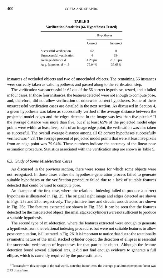
instances of occluded objects and two of unoccluded objects. The remaining 66 instanceswere correctly taken as valid hypotheses and passed along to the verification step.
The verification was successful in 62 out of the 66 correct hypotheses tested, and it failedin four cases. In those four instances, the features detected were not enough to compute pose,and, therefore, did not allow verification of otherwise correct hypotheses. Some of theseunsuccessful verification cases are detailed in the next section. As discussed in Section 4,a given hypothesis was taken as successfully verified if the average distance between theprojected model edges and the edges detected in the image was less than five pixels.2 Ifthe average distance was more than five, but if at least 65% of the projected model edgepoints were within at least five pixels of an image edge point, the verification was also takenas successful. The overall average distance among all 62 correct hypotheses successfullyverified was 4.28. The average percent of projected model points that were at least five pixelsfrom an edge point was 79.04%. These numbers indicate the accuracy of the linear poseestimation procedure. Statistics associated with the verification step are shown in Table 5.
6.3. Study of Some Misdetection Cases
As discussed in the previous section, there were scenes for which some objects werenot recognized. In those cases either the hypothesis-generation process failed to generatesuitable hypotheses or the verification procedure failed due to a lack of suitable featuresdetected that could be used to compute pose.
An example of the first case, where the relational indexing failed to produce a correcthypothesis is illustrated in Fig. 25. The original right image and edges detected are shownin Figs. 25a and 25b, respectively. The primitive lines and circular arcs detected are shownin Fig. 25c. The features extracted are shown in Fig. 25d. It can be seen that the featuresdetected for the misdetected object (the small stacked cylinder) were not sufficient to producea suitable hypothesis.
The second type of misdetection, where the features extracted were enough to generatea hypothesis from the relational indexing procedure, but were not suitable features to allowpose computation, is illustrated in Fig. 26. It is important to notice that due to the rotationallysymmetric nature of the small stacked cylinder object, the detection of ellipses is essentialfor successful verification of hypotheses for that particular object. Although the featuredetection found several elliptical arcs, it did not find enough evidence to generate a fullellipse, which is currently required by the pose estimator.
2 To transform this concept to the real world, note that in our tests, the average pixel/mm conversion factor was2.43 pixels/mm.
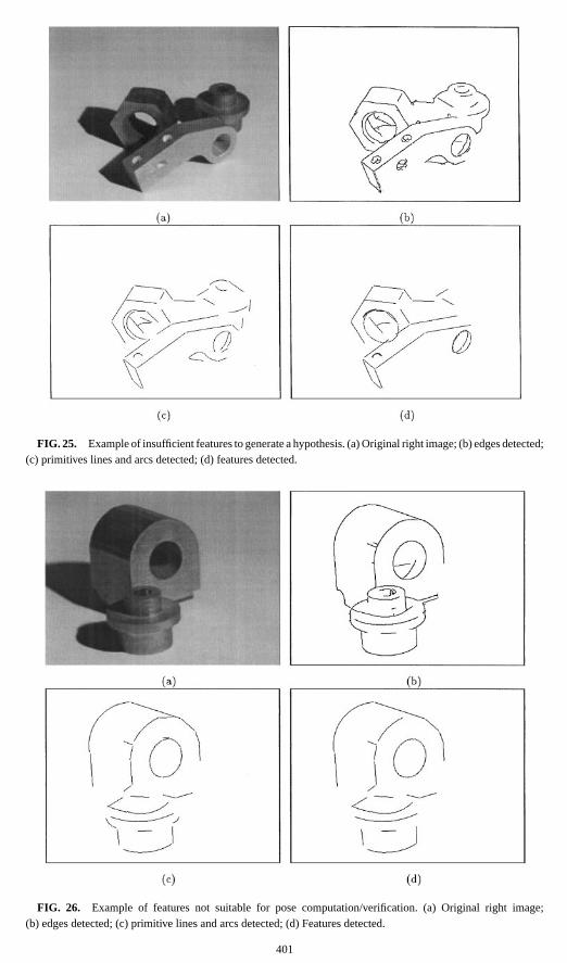
FIG. 25. Example of insufficient features to generate a hypothesis. (a) Original right image; (b) edges detected;(c) primitives lines and arcs detected; (d) features detected.
FIG. 26. Example of features not suitable for pose computation/verification. (a) Original right image;(b) edges detected; (c) primitive lines and arcs detected; (d) Features detected.
401
402 COSTA AND SHAPIRO
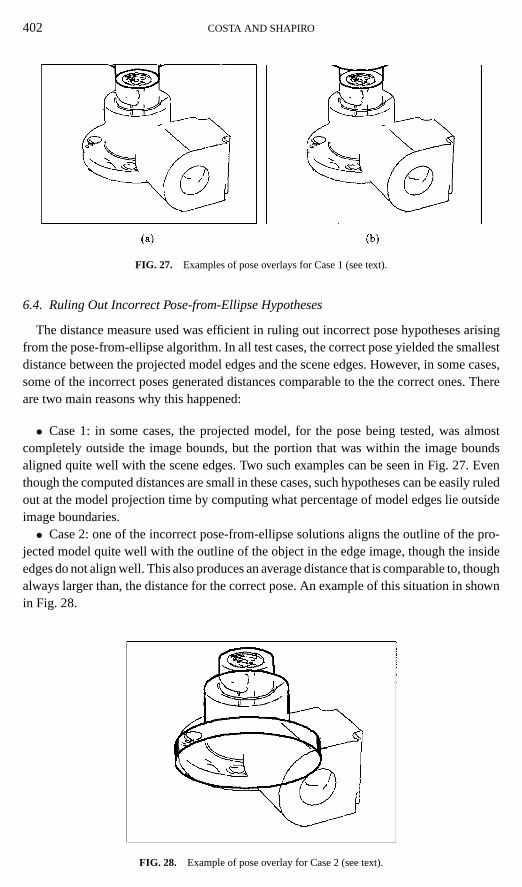
FIG. 27. Examples of pose overlays for Case 1 (see text).
6.4. Ruling Out Incorrect Pose-from-Ellipse Hypotheses
The distance measure used was efficient in ruling out incorrect pose hypotheses arisingfrom the pose-from-ellipse algorithm. In all test cases, the correct pose yielded the smallestdistance between the projected model edges and the scene edges. However, in some cases,some of the incorrect poses generated distances comparable to the the correct ones. Thereare two main reasons why this happened:
• Case 1: in some cases, the projected model, for the pose being tested, was almostcompletely outside the image bounds, but the portion that was within the image boundsaligned quite well with the scene edges. Two such examples can be seen in Fig. 27. Eventhough the computed distances are small in these cases, such hypotheses can be easily ruledout at the model projection time by computing what percentage of model edges lie outsideimage boundaries.• Case 2: one of the incorrect pose-from-ellipse solutions aligns the outline of the pro-
jected model quite well with the outline of the object in the edge image, though the insideedges do not align well. This also produces an average distance that is comparable to, thoughalways larger than, the distance for the correct pose. An example of this situation in shownin Fig. 28.
FIG. 28. Example of pose overlay for Case 2 (see text).

3D OBJECT RECOGNITION AND RELATIONAL INDEXING 403
TABLE 6
Average Distancesd from Pose-from-Ellipse Algorithm
Test image Correct pose Pose 2 Pose 3 Pose 4
1 4.232169 5.905406 38.015209 38.0641822 3.492276 3.836853 5.438044 6.2295563 2.565156 10.072806 75.727005 77.7690814 6.048713 6.095455 7.518664 9.9847725 6.500802 10.659150 12.863460 14.9709146 4.760042 5.682881 37.694584 38.2043767 3.650602 4.853358 22.808851 23.7144788 5.016474 7.895664 45.042072 51.1290519 3.737756 9.964845 15.774166 21.634424
10 5.117007 10.208114 82.480644 84.06028711 6.213883 10.301037 90.775963 92.62401612 2.749343 4.488708 6.710792 11.89696213 6.487325 15.678705 45.408619 49.99157714 1.485621 11.119739 14.899862 18.39723615 5.114830 11.136388 12.420178 14.751463
Table 6 shows the distance measure computed for each four possible pose cases for 15different test images. In all cases, the correct pose yielded the smallest distance.
6.5. Improving the Verification of Occluded Object Hypotheses
It can be seen from the data shown in Fig. 24b that a large part of the projected modeledges do not align well with the scene edges due to the fact that the corresponding portion ofthe model is occluded by another object. Therefore, it is apparent that occlusion adverselyaffects the verification procedure devised. In order to make the verification more effectivefor occluded objects, the following steps may be added to it. First, all unoccluded objectsare identified. This can be done not only by means of the distance measure (d) and thepercentage of points that align well (p), but also from the pose parameters themselveswhich include the exact 3D location of each object. Thus, it is possible to determine whichobjects in the scene are occluded by one or more object. Once the unoccluded objects havebeen identified, their corresponding projected edges are used to generate masks. The masksgenerated for the case study introduced in Section 5.2 can be seen in Figs. 29a and 29b.These masks are used to mask out the predicted occluded regions in the projected model ofthe occluded object as shown in Fig. 29d. Then the masked project model is used to computed and p, which will determine whether the verification succeeds or not. It is shown in thecaptions of Figs. 29e and 29f that bothd andp are greatly improved by this masking process,making the verification more reliable.
7. DISCUSSION AND FUTURE WORK
This paper described the RIO object recognition system. RIO utilizes a number of newtechniques to recognize 3D objects in 2D intensity images. Real images are used in thestage of learning the feature-based relational models of the objects to be recognized. Anew technique called relational indexing is used as an effective database retrieval tool,generating suitable model hypotheses. A new linear pose estimation technique is used to
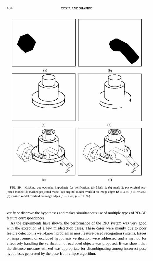
404 COSTA AND SHAPIRO
FIG. 29. Masking out occluded hypothesis for verification. (a) Mask 1; (b) mask 2; (c) original pro-jected model; (d) masked projected model; (e) original model overlaid on image edges (d = 3.84, p = 79.5%);(f ) masked model overlaid on image edges (d = 2.42, p = 91.3%).
verify or disprove the hypotheses and makes simultaneous use of multiple types of 2D–3Dfeature correspondences.
As the experiments have shown, the performance of the RIO system was very goodwith the exception of a few misdetection cases. These cases were mainly due to poorfeature detection, a well-known problem in most feature-based recognition systems. Issueson improvement of occluded hypothesis verification were addressed and a method foreffectively handling the verification of occluded objects was proposed. It was shown thatthe distance measure utilized was appropriate for disambiguating among incorrect posehypotheses generated by the pose-from-ellipse algorithm.

3D OBJECT RECOGNITION AND RELATIONAL INDEXING 405
Even though the verification procedure was proven to be reliable given the criterion used,namely the average distance between projected CAD model edges and scene edges andthe percentage of projected edge pixels that aligned well with scene edge pixels, it is feltthat a more robust verification criterion needs to be developed. Making the assumption thatthe distances between projected model edge points and scene edge points have a Gaussiandistribution, it seems logical to use a chi-squared test (with as many degrees of freedom asthe points in the projected model edges) to decide whether or not the alignment producedby the computed pose is acceptable.
All the experiments run were limited to subgraphs of size 2. As mentioned in Section 4,the smallest size index was used in order to effectively handle occlusion. However, a hier-archical, multilevel indexing approach is also viable and should be investigated. The largerthe subgraphs used, the more reliable the generated hypotheses will be, and the faster theycan be generated. However, in multiobject scenes only single features or small subgraphsmay be detected. Therefore, it is necessary to start at the largest subgraph level and go downas needed. Objects that are unoccluded may be recognized at the highest level of indexing.
Work on investigating the effects of occlusion on the single-object feature-based modelsis in order. The special case of multiple-object scenes that contain a considerable amountof occlusion needs to be studied carefully. It is intuitive that the set of features that can bereliably detected from a real image of a particular model alone is a superset of the features thatcan be detected in a scene where that model is partially occluded. The technique developedwas designed to handle occlusions. However, when the object is partially occluded, it ispossible that some of the original features detected in its training images can change andgive rise to new features that often appear when occlusion is present. It is also possible thatnew relationships between features arise due to occlusion. It seems logical to augment thecurrent single-object feature-based models to include the knowledge obtained by studyinga set of training images where multiple objects and occlusion are present.
A discrete voting technique was associated with the relational indexing method devel-oped in this work. Relational indexing can be performed in the context of a probabilisticframework, as described in [14]. This should considerably improve the hypotheses gen-erated, since the probabilities associated with the features (computed at model generationtime) can be used as weights when computing the votes to be cast.
REFERENCES
1. J. Ben-Arie and A. Z. Meiri, 3-d object recognition by optimal matching search of multinary relations,Comput.Vision Graphics Image Process.37, 1987, 345–361.
2. R. Bergevin and M. D. Levine, Generic object recognition: Building and matching coarse descriptions fromline drawings,IEEE Trans. Pattern Anal. Mach. Intell.15, 1993, 19–36.
3. J. P. Besl and R. C. Jain, Three-dimensional object recognition,ACM Comput. Surveys17, 1985, 75–154.
4. R. C. Bolles and R. A. Cain, Recognizing and locating partially visible objects: The local-feature-focusmethod,Int. J. Robotics Res.1(3), 1982, 57–82.
5. R. C. Bolles and P. Horaud, 3dpo: A three-dimensional part orientation system,Int. J. Robotics Res.5(3),1986, 3–26.
6. J. P. Brady, N. Nandhakumar, and J. K. Aggarwal, Recent progress in object recognition from range data,Image Vision Comput.7(4), 1989, 295–307.
7. J. B. Burns and E. M Riseman, Matching complex images to multiple 3d objects using view descriptionnetworks, inProc. of the IEEE CVPR, pp. 328–334, 1992.

406 COSTA AND SHAPIRO
8. A. Califano and R. Mohan, Multidimensional indexing for recognition of visual shapes,IEEE Trans. PatternAnal. Mach. Intell.16, 1994, 373–482.
9. O. I. Camps, L. G. Shapiro, and R. M. Haralick, Image prediction for computer vision, inThree-dimensionalObject Recognition Systems(A. Jain and P. Flynn, Eds.), Elsevier, Amsterdam/New York, 1993.
10. C. H. Chen and A. C. Kak, A robot vision system for recognizing 3d objects in lower order polynomial time,IEEE Trans. Systems Man Cybernetics19, 1989, 1535–1563.
11. C. H. Chen and P. Mulgaonkar, Automatic vision programming,CVGIP: Image Understanding55, 1992,170–183.
12. J. L. Chen and G. C. Stockman, Matching curved 3d object models to 2d images, inSecond CAD-Based VisionWorkshop(A. Kak and K. Ikeuchi, Eds.), pp. 210–227, 1994.
13. R. T. Chin and C. R. Dyer, Model-based recognition in robot vision,ACM Comput. Surveys18, 1986, 67–108.
14. Y. Chou and L. G. Shapiro, Probabilistic relational indexing, inProceedings of the International Conferenceon Pattern Recognition, Brisbane, Australia, 1997, pp. 1331–1335, 1998.
15. M. S. Costa, R. M. Haralick, and L. G. Shapiro, Optimal affine invariant point matching, inProceedings of10th ICPR, Vol. 1, pp. 233–236, 1990.
16. M. S. Costa and L. G. Shapiro, Scene analysis using appearance-based models and relational indexing, inInternational Symposium on Computer Vision, November 1995, pp. 103–108.
17. M. S. Costa,Object Recognition and Pose Estimation Using Appearance-Based Features and RelationalIndexing, Ph.D. Dissertation, Department of Electrical Engineering, University of Washington, 1997.
18. M.-P. Dubuisson and A. K. Jain, A modified Hausdorff distance for object matching, inProceedings of the12th International Conference on Pattern Recognition, Jerusalem, Israel, 1994.
19. W. H. Presset al., Numerical Recipes in C, Cambridge Univ. Press, Cambridge, UK, 1992.
20. D. Forsythet al., Invariant descriptors for 3-d object recognition and pose,IEEE Trans. Pattern Anal. Mach.Intell. 13, 1991, 971–991.
21. M. Dhomeet al., Spatial localization of modeled objects of revolution in monocular perspective vision, inFirst European Conference on Computer Vision, 1989.
22. C. Dorai and A. K. Jain, Shape spectrum based view grouping and matching of 3D free-form objects,IEEETrans. Pattern Anal. Mach. Intell.19, 1997, 1131–1138.
23. A. Etemadi, Robust segmentation of edge data, inProceedings of the IEE Image Processing Conference, 1992.
24. T. J. Fan, G. Medioni, and R. Nevatia, Recognizing 3d objects using surface descriptions,IEEE Trans. Patt.Anal. Mach. Intell.11, 1989, 1140–1157.
25. O. D. Faugeras,Three-Dimensional Computer Vision, a Geometric Viewpoint, MIT Press, Cambridge, MA,1993.
26. O. D. Faugeras and M. Hebert, The representation, recognition, and locating of 3d objects,Int. J. RoboticsRes.5(3), 1986, 27–52.
27. P. J. Flynn and A. K. Jain, Bonsai: 3d object recognition using constrained search,IEEE Trans. Pattern Anal.Mach. Intell.13, 1991, 1066–1075.
28. S. Ganapathy, Decomposition of transformation matrices for robot vision, inProceedings of the InternationalConference on Robotics and Automation, 1984.
29. C. Goad, Fast 3D model-based vision, inFrom Pixels to Predicates(A. P. Pentland, Ed.), pp. 371–391, 1986.
30. K. D. Gremban and K. Ikeuchi, Appearance-based vision and the automatic generation of object recognitionprograms, inThree-dimensional Object Recognition Systems(A. Jain and P. Flynn, eds.), Elsevier, Amster-dam/New York, 1993.
31. L. Grewe and A. Kak, Interactive learning of multiple attribute hash table for fast 3d object recognition, inProceedings of the Second CAD-Based Vision Workshop, February 1994, pp. 124–131.
32. R. M. haralick, C. N. Lee, K. Ottenburg, and M. Nolle, Review and analysis of the three-point perspectivepose estimation problem,Int. J. Comput. Vision13, 1994, 331–356.
33. R. M. Haralick and L. G. Shapiro,Computer and Robot Vision, Addison-Wesley, Reading, MA, 1993.
34. I. Higuchi, H. Delingette, M. Hebert, and K. Ikeuchi, Merging multiple views using a spherical representation,in Proceedings of the Second CAD-Based Vision Workshop, February 1994, pp. 124–131.

3D OBJECT RECOGNITION AND RELATIONAL INDEXING 407
35. D. P. Huttenlocher,Three-Dimensional Recognition of Solid Objects from a Two-Dimensional Image, Ph.D.dissertation, Massachusetts Institute of Technology, 1988.
36. D. P. Huttenlocher and S. Ullman, Recognizing solid objects by alignment with an image,Int. J. Comput.Vision5, 1990, 195–212.
37. K. Ikeuchi and T. Kanade, Towards automatic generation of object recognition programs,CVGIP: ImageUnderstanding76, 1988, 1016–1035.
38. A. K. Jain and R. Hoffman, Evidence-based recognition of 3-d objects,IEEE Trans. Pattern Anal. Mach.Intell. 10, 1988, 783–802.
39. Q. Ji, M. S. Costa, R. M. Haralick, and L. G. Shapiro, An integrated technique for pose estimation fromdifferent geometric features, inProceedings of Vision Interface ’98, Vancouver, June 18-20, 1998, pp. 77–84.
40. A. E. Johnson and M. Hebert, Efficient multiple model recognition in cluttered 3-D scenes, inProceedings ofthe IEEE Conference on Computer Vision and Pattern Recognition, 1998, pp. 671–677.
41. Y. Lamdan and H. J. Wolfson, Geometric hashing: A general and efficient model-based recognition scheme,in Second International Conference on Computer Vision, pp. 238–249, 1988.
42. D. G. Lowe, Three-dimensional object recognition from single two-dimensional images,Artificial Intell. 31,1987, 355–395.
43. H. Murase and S. K. Nayar, Visual learning of object models from appearance,Int. J. Comput. Vision14(1),1995, 5–24. [Also Technical Report CUCS-054-92]
44. C. F. Olson, Probabilistic indexing for object recognition,IEEE Trans. Pattern Anal. Mach. Intell.17, 1995,518–522.
45. T. Q. Phong, R. Horaud, A. Yassine, and P. D. Tao, Objet pose from 2-d to 3-d point and line correspondences,Int. J. Comput. Vision15, 1995, 225–243.
46. A. R. Pope,Model-based Object Recognition—A Survey of Recent Research, Technical Report 94-04, January1994.
47. K. Pulli, Triplet-based object recognition using synthetic and real probability models, inProceedings ofICPR96, 1996, Vol. IV, pp. 75–79.
48. M. Seibert and A. M. Waxman, Adaptive 3d object recognition from multiple views,IEEE Trans. PatternAnal. Mach. Intell.14, 1992, 107–124.
49. L. G. Shapiro and R. M. Haralick, A metric for comparing relational descriptions,IEEE Trans. Pattern Anal.Mach. Intell.7, 1985, 90–94.
50. F. Stein and G. Medioni, Structural indexing: Efficient three dimensional object recognition,IEEE Trans.Pattern Anal. Mach. Intell.14, 1992, 125–145.
51. G. Stockman, Object recognition and localization via pose clustering,Comput. Vision Graphics Image Process.40, 1987, 361–387.
52. T. M. Strat and M. A. Fishler, Contex-based vision: recognizing objects using information from both 2d and3d imagery,IEEE Trans. Pattern Anal. Mach. Intell.13, 1991, 1050–1065.
53. P. Suetens, P. Fua, and A. J. Hanson, Computational strategies for object recognition,ACM Comput. Surveys24, 1992, 5–61.
54. K. B. Thornton,Clustering Similar Views of an Object Using a Relational Distance Approach, Master’s thesis,1989.
55. R. Y. Tsai, An efficient and accurate camera calibration technique for 3d machine vision,IEEE J. RoboticsAutomation3(4), 1987, 323–344.
56. R. C. Bolles and P. Horaud, 3DPO: a three-dimensional part orientation system,Int. J. Robotics Res.5(3),1986, 3–26.
57. L. B. Wolff, Polarization-based material classification from specular reflection,IEEE Trans. Pattern Anal.Mach. Intell.12, 1990, 1059–1071.
58. A. K. C. Wong, L. Rong, and X. Liang, Robotic vision: 3D object recognition and pose determination, inProceedings of the 1998 IEEE/RSJ International Conference on Intelligent Robots and Systems, pp. 1202–1209, 1998.
59. S. Zhang, G. D. Sullivan, and K. D. Baker, The automatic construction of a view-independent relational modelfor 3d object recognition,IEEE Trans. Pattern Anal. Mach. Intell.15, 1993, 531–544.