1

3D numerical modeling of flow along spillways with free surface flow. Complementary spillway of Salamonde.

Miguel Rocha Silva Instituto Superior Técnico, Civil Engineering Department

1. INTRODUCTION Throughout the design and planning for hydraulic structures as spillways, some technical decisions are often supported by assessing the flow behavior in physical models. However, engineers and researchers are increasingly integrating computational fluid dynamics (CFD) into the process. Despite reports of success in the past, there is still no comprehensive assessment that assigns ability to CFD models to simulate a wide range of different spillways configurations. In this study, the applicability of a commercial CFD model (FLOW-3D) to simulate the flow into a geometry complex spillway was reviewed.

To solve the governing equations of fluid flow, FLOW-3D solves a modification of the commonly used Reynolds Average Navier-Stokes (RANS) equations. Additionally, the software include algorithms to track the free surface (VOF method) and represent the geometrical details (FAVOR).

2. OBJECTIVES The main objective of the present study is to evaluate how accurately the FLOW-3D could represent the flow characteristics (e.g. velocity, pressure, flow depths) a complex spillway and help engineers to make some technical decisions. Further, there are secondary objectives related to calibration and validation of the numerical model such as:

• Calibrate the computational model, providing a sensitive analysis for some of the main parameters/models in FLOW-3D;

• Validate the computational model using physical model discharge and flow depths measurements;

• Assess the computational model results for design conditions and compare them with the physical model.

3. CALIBRATION OF THE COMPUTATIONAL MODEL

The calibration and validation of numerical models are extremely important and therefore it constitutes part of the analysis tasks in most of the CFD models. In fact, an on-going effort to carry out validation against published or experimental data remains essential. This is really important to ensure modeling correctness and to provide a high confidence level in its application.

3.1. Case study and physical model

Salamonde dam, located in the north of Portugal in river Cávado, Peneda Gerês National Park, is a double-curved arch dam in concrete with maximum height of 75 m from foundation. After safety analysis from (EDP, 2006), it was concluded that it would be necessary an additional

2

discharge structure – the complementary spillway for Salamonde dam (under construction), which is the case study in this study

The complementary spillway of Salamonde dam, is a gated spillway, controlled by an ogee crest, followed by a tunnel with rather complex geometry, designed for free surface flow, and a ski jump structure which directs the jet into the river bed. The ogee crest is divided into two spans controlled by radial gates, with 6.50 m wide each. The design discharge for this structure is 1233 m3/s, corresponding to a level of 270,64 m in the reservoir.

The outlet structure is a ski jump, producing a free jet with impinging region in the center of the river bed. Along the last 28 m of the outlet structure, the spillway cross-section is progressively reduced, to increase jet height, and consequently, the length of the impact area

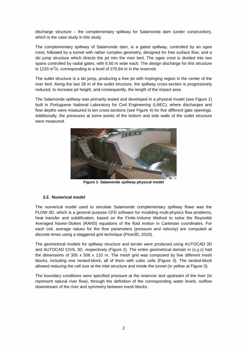
The Salamonde spillway was primarily tested and developed in a physical model (see Figure 1) built in Portuguese National Laboratory for Civil Engineering (LNEC), where discharges and flow depths were measured in ten cross-sections (see Figure 4) for five different gate openings. Additionally, the pressures at some points of the bottom and side walls of the outlet structure were measured.

Figure 1- Salamonde spillway physical model

3.2. Numerical model

The numerical model used to simulate Salamonde complementary spillway flows was the FLOW-3D, which is a general purpose CFD software for modeling multi-physics flow problems, heat transfer and solidification, based on the Finite-Volume Method to solve the Reynolds Averaged Navier-Stokes (RANS) equations of the fluid motion in Cartesian coordinates. For each cell, average values for the flow parameters (pressure and velocity) are computed at discrete times using a staggered grid technique (Flow3D, 2010).

The geometrical models for spillway structure and terrain were produced using AUTOCAD 3D and AUTOCAD CIVIL 3D, respectively (Figure 2). The entire geometrical domain in (x,y,z) had the dimensions of 305 x 506 x 110 m. The mesh grid was composed by five different mesh blocks, including one nested-block, all of them with cubic cells (Figure 3). The nested-block allowed reducing the cell size at the inlet structure and inside the tunnel (in yellow at Figure 3).

The boundary conditions were specified pressure at the reservoir and upstream of the river (to represent natural river flow), through the definition of the corresponding water levels, outflow downstream of the river and symmetry between mesh blocks.

3

Figure 2- Salamonde spillway 3D geometric Figure 3- Computational domain

3.3. Sensitive analysis based of the physical model discharge results

Firstly, a sensitive analysis of the main models/configurations in FLOW-3D based on the physical model discharge results was carried out. The model configurations under analysis were:

• Momentum advection model (1st order vs 2nd order with monotonicity preserving (MP));

• VOF method (Default vs Split Lagragian Method); • Turbulence mixing length (TLEN) parameter; • Cell size.

In this analysis, three different discharges were considered by setting the level in the reservoir (Table 1)

Table 1- Physical model discharges for three defined reservoir levels

Reservoir level QPhysical Model

(m) (m3/s)

260.43 100.0

262.47 250.0

267.05 750.0

It is important to refer that every simulations were considered with a 1.00 m cell size (coarsest mesh capable to solve the flow) and for 200 s (except for cell size analysis, where Restart simulations were performed for 30 s). The results of flow rate presented are calculated as an average value after steady state was attained.

Due to the high volume of results, only the ones referring to the first simulation (with default FLOW-3D configurations) and after sensitive analysis (named 2nd simulation) will be presented:

1st Simulation configurations: 2nd Simulation configurations: • 1st order momentum advection method • 2nd order with MP momentum advection

method • Default VOF Method • Default VOF Method • Laminar regime • RNG turbulence model

• TLEN = 0.4 m • Cell size: 1.0 m • Cell size: 0.25 m

4

The numerical results are presented in Table 2. Additionally, the differences to physical model results are shown.

Table 2 – Numerical model discharges

Reservoir level QPhysical Model 1st simulation 2nd simulation

(m) (m3/s) QCFD (m3/s) Diff. (%) QCFD (m3/s) Diff. (%)

260.43 100.0 81.9 -18.1 90.1 -9.9

262.47 250.0 223.1 -10.8 235.2 -5.9

267.05 750 690.3 -8.0 729.6 -2.7

Up to more accurate configurations presented above as 2nd simulation, several combinations of parameters were tested with FLOW-3D, resulting in 14 as a total number of simulations. Throughout this process, some main conclusions were obtained:

• 2nd order momentum advection with monotonicity preserving showed more accurate results without much more computational effort;

• Split Lagrangian VOF had almost no influence on the discharge results and needed significantly more computational effort;

• The transition from a laminar regime model to a turbulence one had, naturally, influence the discharge results. Discharges were, as expected, lower after RNG turbulence model was used;

• The turbulence mixing length parameter (TLEN) had huge importance in the simulation stability and duration. However, it had not significant influence on discharge values.

• The obtained discharges were highly dependent on cell size.

3.4. Sensitive analysis based of the physical model flow depths measurements

In the second phase of the calibration of the computational model, flow depths from physical and numerical model were compared. In the physical model, flow depths were measured in ten cross-sections (Figure 4) for five different gate openings. The results used to calibrate the numerical model were the ones corresponding to symmetric gates openings of 2.00 m. In this flow conditions, the physical model discharge was 267.0 m3/s.

Figure 4 - Location of the ten cross-sections for f low depth measurements (LNEC, 2012)

The model configurations under analysis were:

• Cell size; • VOF method (Default vs Split Lagragian Method); • Turbulence mixing length (TLEN) parameter.

5

The physical and computational flow depths results are compared in Figure 5. Due to the high volume of results, the ones presented are related to the cell size sensitive analysis. It is important to refer that the presented results are related to restart simulations from steady state conditions.

Section 1 Section 2 Section 3

Section 4 Section 5 Section 6

Section 7 Section 8 Section 9

Section 10 Figure 5 – Flow depths for numerical and physical m odels

The results showed that for 0.25 m cell size, FLOW-3D was able to represent accurately the flow depths although underpredicts the highest values near the walls (particularly in sections 5 and 7). Clearly, the 1.00 m cell size has proved insufficient to represent accurately the flow behavior and the geometric details of the structure.

The numerical flow rate results are presented in Table 3 as a function of cell size.

6

Table 3 – Numerical model discharges as a function of the cell size

Cell size (m)

1.00 0.50 0.25

QPhysical Model (m3/s) QFLOW-3D (m3/s) Diff. (%) QFLOW-3D

(m3/s) Diff. (%) QFLOW-3D (m3/s)

Diff. (%)

267.0 207.8 -22.2 239.2 -10.4 259.5 -2.8

The results presented in Table 3 show an increased accuracy for reduced mesh size simulations.

Referring to the VOF method sensitive analysis, the Split Lagragian VOF method was not able to reproduce the highest flow depths near the walls and the computational time was significantly increased. Additionally, the flow rate results were almost independent of the VOF method. Therefore, the Default VOF method was considered for further simulations.

Regarding TLEN parameter sensitive analysis, this had neither influence in flow depths nor flow rate results. The dynamically computed option of TLEN parameter (default option) did not appear to be a reasonable choice since it drastically increased the computational time.

4. RESULTS FOR DESIGN DISCHARGE CONDITIONS

After a calibrated and validated numerical model, the design discharge condition was simulated and the corresponding results were assessed. The FLOW-3D main configurations were:

• 2nd order monotonicity preserving momentum advection; • Default VOF (One fluid, free surface); • RNG turbulence model; • TLEN adjusted in real time (between 0,4 and 0,1 m); • Cell size 0,50 m and 0,25 m for Restart simulation.

The simulations and real computational time were:

1st simulation : cell size 0.50 m for 60 s corresponding to a real simulation time of 21:27 h;

2nd simulation (Restart simulation): cell size 0.25 m for 10 seconds corresponding a real simulation time of 17:05 h.

The computational discharges calculated in the first simulation are presented in Figure 6. After steady state was attained, the average computational discharge was 1206.5 m3/s, corresponding to a difference of -2.15% to the design value.

7

Figure 6 - Calculated discharge in 1 st simulation

Due to the importance of having a global perception of the flow behavior and its main characteristics, the following topics were more carefully studied:

• Inlet structure analysis (qualitatively); • Flow depths; • Velocity; • Pressure; • Asymmetric gates openings (qualitatively); • Free jet; • Water level fluctuations against the slopes of the valley.

4.1. Inlet structure analysis

The analysis of water flow in an inlet structure of a spillway is an important engineering problem. In fact, favorable approach flow conditions should be provided to the spillways in order to avoid reduced discharge capacity.

An analogy between the physical and computational models for the inlet structure is presented in Figures 7 and 8.

Figure 7 – Physical model inlet structure Figure 8 – Numerical model inlet structure

Figure 7 shows a slight flow separation along the pier and the guide walls, which is somehow simulated by the numerical model (Figure 8).

8

4.2. Flow depths

A quantitative flow depths analysis was carried out by comparing the numerical model results to the design ones. It is important to notice that in design phase, the mean flow depths at certain cross-sections were calculated by using a simple 1D model which considers simplifications such as hydrostatic pressure distribution along the whole spillway.

The average flow depths were analyzed in the ten cross-sections defined and presented in Figure 4. For the Sections 1 and 2, the numerical model overpredicted significantly the average fluid depth comparatively to the design values (values 40 % higher). In this region, the flow is extremely accelerated so, an hydrostatic pressure is not expected. It is believed that 1D model results are not a good term of comparison for this kind of flow conditions.

For the other analyzed cross-sections, the numerical model came up with more accurate results, with an average difference of around 10 % to the design average flow depths.

4.3. Velocity

Additionally, average velocity numerical results were compared with design ones. The post-processing software EnSight was used to render the velocity profiles (Figure 9) in the cross sections presented in Figure 9. Then, the velocity spatial mean value was calculated using an intern function in the software.

Figure 9 – Velocity profile in Section 6 (rendered wi th EnSight)

Numerical model average velocity results showed differences of around -11 % for all ten cross-sections, comparing to the design values. These minor differences can be in part explained by the non-uniform velocity profiles in the FLOW-3D, contrasted with the 1D model. Indeed, in the 1D model, uniform velocity profiles are considered. Therefore, it is believed that FLOW-3D can accurately represent the real velocity along the spillway.

4.4. Pressure

One of the greatest benefits of CFD models is the possibility to determine the main characteristics of the flow in any region of the computational domain. In order to assess the ability of FLOW-3D to support the design phase, a quantitative pressure analysis was developed.

9

One of the main reasons for building the physical model was to allow pressure measurements at the outlet structure. In the numerical model, pressure diagrams were rendered for each 5 m (Figure 9). Figure 9 shows, clearly, a structural conditioning section.

Figure 9 – Pressure diagrams in the outlet structure

In the physical model, several pressure tapping points were considered in the bottom and side walls of the outlet structure. For a quantitative analysis between physical and numerical models, four different points were selected (two in the bottom wall and two for the right wall)

Figure 10 – Pressure diagram at 10.20 m from

downstream outlet structure limit Figure 11 – Pressure diagram at 2.00 m from

downstream outlet structure limit

Figure 10 shows the cross-section where the highest pressure values were measured. In the physical model, the highest pressure was measured at point 2F (16.13 m water depth ≈ 158181 Pa). For this same point, pressure value calculated at the numerical model presents only a 0.4% difference (158747 Pa – Figure 10). For the remaining compared pressure tapping points (points 1, 3 and 1F), an average difference of -12.6% from numerical and physical models was achieved. It must be pointed out that hydrostatic pressure measurement is prone to errors in physical models due to slight imperfections in tap orientation relatively to the walls surfaces.

P2F

P3

P1

P1F

10

4.5. Asymmetric gates openings

In the design phase of spillway structures, is often considered the hypothetical scenario of failure of one of the gates. Therefore, this same scenario was qualitatively analyzed in the physical model. Due to asymmetry of the Salamonde spillway, two different scenarios were analyzed: right gate failure and left gate failure.

These same qualitative analyzes were performed in the numerical model. The results presented in Figures 12 and 13 refer to the failure of right gate. This proved to be the worst case scenario since it showed significant flow projections on the right side wall of the spillway, downstream of the septum (see Figure 13).

Figure 12 – Flow pattern for right gate failure Figure 13 – View of the tunnel from downstream

4.6. Free jet

One of the main objectives of building the physical model of the Salamonde spillway was to assess the free jet impinging region at the river bed. In fact, in this kind of outlet structures with ski jump, engineers are concerned to direct the free jet impingement to the center of the river bed to avoid significant erosions on the river banks.

Figure 14 – Free jet. Physical model Figure 15 – Free jet. Numerical model

11

A qualitative analysis was performed with the numerical model. In Figures 14 and 15, an comparison of jet configuration between physical and numerical models is presented. From the several physical model photos evaluated, FLOW-3D appears to represent accurately the shapes of the free jet.

Additionally, a quantitative analysis was carried out. The numerical results for minimum and maximum impingement of the free jet were compared with the measurements in the physical model and are presented in Table 4.

Table 4 – Free jet impingement distance results

Physical model FLOW-3D Diff. (%)

Minimum impingement distance (m) 49.0 48.5 -1.0%

Maximum impingement distance (m) 91.0 68.4 -24.9%

Comparing to physical model results, numerical model accurately represented the minimum free jet impingement, with a -1.0% difference. For its maximum value, the difference was significantly higher. In part, this difference could be explained by the lack of air entrainment model consideration in FLOW-3D.

4.7. Water level fluctuations against the slopes of the valley

One of the major concerns of engineers during the design of spillways with free jet dissipation is the increase of the level in the river slopes. FLOW-3D could help to decide the jet impinging region in the river bed in order to minimize erosion and water level fluctuations against the slopes of the valley.

Water level fluctuations against the slopes of the valley are shown, after steady state was reached are shown in Figure 16. For Salamonde complementary spillway design discharge, a 12 m elevation above the maximum river level was expected.

Figure 16 – Water level fluctuations against the sl opes of the valley

12

5. CONCLUSIONS

The main conclusion from the present study is that, in general, FLOW-3D accurately represents the flow along the spillway with rather complex geometry, referring to its behavior and main characteristics such as flow rates, velocity, pressure and flow depths.

Nevertheless, there are several aspects that should be considered to obtain more accurate results. A sensitive analysis for some main FLOW-3D configurations and parameters is highly recommended before starting to predict flow characteristics.

In the present work, the 2nd order momentum advection model with monotonicity preserving was a good choice for better accuracy without much more computational time. Split Lagragian VOF did not appear to be useful in this kind of extreme velocity flow conditions. As referred in Lan (2010) and Dargahi (2010), the turbulence mixing length parameter (TLEN) has a huge importance in simulation stability and duration. The rule of thumb of 7% referred in (FLOW-3D, 2010) appears to be a good estimate for this parameter value. However it is recommended that a sensitive analysis to this parameter should be done in each case study. The numerical results showed to be highly dependent of the cell size. In fact, smaller cells allow reproducing geometric details such as complex cross-sections and radial gates.

FLOW-3D can be very useful for structural design of hydraulic structures. Pressure diagrams and velocity profiles can be rendered with a post-processing software and can be helpful in that design phase.

REFERENCES

Dargahi, B., 2010. Flow characteristics of bottom outlets with moving gates. Journal of Hydraulic Research, 48(4):476–482, 2010. EDP, 2006. Barragem de Salamonde: Controlo da segurança hidráulico operacional; revisão do estudo das cheias e análise da adequação dos órgãos de descarga. Technical report, EDP, Portugal. Flow-3D, 2010. Flow-3D User Manual, Version 10.0. Flow Science, Inc., 10 edition. Lan, F., 2010. CFD assisted spillway and stilling basin design. In FLOW-3D Flow Simulation Contest. Flow Science, Inc. LNEC, 2012. Modelação do escoamento no canal do descarregador de cheias complementar da barragem de Salamonde - observações em modelo reduzido. Technical report, Laboratório Nacional de Engenharia Civil (LNEC), Outubro 2012.