3D MR Image Denoising Using higher O rder Kernel Regression

1

Dr. C Nalini1 , A.Gayathri

2,A.Srinivasan

3

1,3Professor,

2Associate Professor,

Computer Science and Engineering,

1BIST, BIHER,Bharath University,Chennai – 73.

2,3Misrimal Navajee Munoth Jain Engineering College, Chennai, 600 097, India

[email protected]

ABSTRACT

Noise removal from images is among the challenging processes for researches. Image denoising is a crucial step to improve 3D

image conspicuity and to enhance the performance of all the processing needs of quantitative image analysis. Magnetic

Resonance (MR) imaging has an increasing importance in the field of medical diagnosis. MR 3D image de-noising has two

features (i) tri-dimensional structure of images and (ii) the nature of the noise, which are Rician & Gaussian. Kernel regression

is one of 3D non-parametric noise level estimation technique which is effective than other denoising experimental filters. The

proposed Fourth order Kernel Regression (FKR) algorithm builds an efficient and robust estimator and improves the accuracy

of noise and it further improves the finer estimations of pixel value and its gradients. Experimental results demonstrate

positively by achieving better performance, with respect to other de-noising filters.

Keywords:

Kernel regression, Median Filter, Medical Images, Rician Noise, Rican Median Absolute Deviation (RMAD) Estimator, Image denoising.

1. INTRODUCTION

Digitalized visual has come to be recognized as the means of

communication in the present era. Images transmitted

digitally are corrupted with noise, hence, have to be denoised

before deploying them in applications [1]. De-noising is done

by manipulating the dataset of received image to produce

high quality images. For removal of noise, knowledge about

the level of noise and the type of noise is vital in selecting the

appropriate de-noising algorithm. Magnetic Resonance

Imaging is an imaging technique to diagnose medical

conditions and the 3D images acquired are corrupted with

noise and makes it difficult for interpretation [2]. This

practical difficulty is usually overcome by reducing the noise

in the images. Usually Rician noise is incorporated in the MR

images [3] and they suffer from a contrast reducing signal

dependent bias. The image used to be enhanced earlier by

modifying the parameters of the MRI device, however, in

these earlier methods, number of test images used for

analyzing is more and hence time consuming [4,5].

Classical image processing parametric methods rely on a

specific model while computing vital parameters. This

process depends on diverse problems ranging from denoising,

up-scaling and interpolation. A generative model based upon

the estimated parameters is then produced as the best estimate

of the underlying signal. Kernel regression is deployed in

order to ascertain the conditional expectation of the noiseless

pixel value with respect to the pixel coordinates of another

image. There are three types of regressions namely

parametric,non-parametric and local polynomial regression.

Parametric regression can be derived as y = f(x) + e, where

known smooth functions is represented as f. In non-

parametric regression f represents unknown smooth function

and is unspecified by regression of modular parametric [6,7].

Weighted Least Squares (WLS) is used by Local polynomial

regression to fit dth degree (d≠0) to data [8]. The weights

assigned to the observations are determined by an “Initial

Kernel Regression Fit” to the data. For image denoising and

enhancement, a non-parametric estimation technique called

kernel regression can be applied successfully.

2. BACKGROUND WORK

Presence of Rician noise in MR intensity images is governed

by Rician distribution. Rayleigh distribution function is used

to generate Rician noise in images mathematically. The

acquired, untreated image data is tainted by Additive White

Gaussian Noise (AWGN), which is a complex value. The

variance σ of the noise is taken as same for both the real and

3D MR Image Denoising Using higher Order

Kernel Regression

International Journal of Pure and Applied MathematicsVolume 119 No. 12 2018, 10877-10889ISSN: 1314-3395 (on-line version)url: http://www.ijpam.euSpecial Issue ijpam.eu

10877

2

assumed complex values [9,10]. MR image is received as a

magnitude of the complex values. The resulting pixels are

therefore corrupted by Rician noise. Let ith pixel of given

image in 3D coordinate represents xi ϵ [1,M] × [1,N] ×[1,P].

Assume ti is true value (noiseless) and qi is observed value

(noisy). The true values of pixel lie in [0, v] range and v =

255 (maximum pixel value).

Two component vectors 2 2( (x )) ( (x ))i i it

, is the

magnitude of ti, where α and χ are real and imaginary values.

The equation of observed value is 2 2( (x ) ) ( (x ) )i i i i iq

which has Rician noise. The

square of the observed value [3, 15] is given by Equation 1 2 2 2[ ] [ ] 2i iE q E t (1)

To achieve best result in terms of robustness and accuracy,

Rician Median Absolute Deviation (RMAD) estimator is

applied primarily, to remove bias from squared magnitude

image and subsequently denoising the magnitude of MR

image. For the images where no background is available, this

estimator is proposed, subject to approximation of Gaussian

noise within the object. The methods for RMAD Estimation

are classified as methods using background areas for

estimating noise variance and image object.

In RMAD estimator equation ti is given by Equation 2

2 2max(0, 2 )i it q (2)

Physically insignificant complex values can be evaded using

maximum function 2 2(x ) t 2i iz

(3) 2

i iy q (4)

3. EXISTING KERNEL REGRESSION

MODULES

Existing image denoising system consists of four modules.

Once the Rician noise level is estimated, a pre-processing

task helps to obtain original image’s gradients and its pilot

estimation. Following this, better inference is ascertained by

deploying the same method. Eventually, the kernel regression

of second order helps to evaluate weights based on filter of

zeroth order. This performance is comparable with Unbiased

Kernel Regression Filter (UKR)

3.1 Rician Noise Estimation

To have reliable estimation of noise level without human

intervention for MR images, this estimation is optimum.

Assuming the noise variance to be the same in both the real

and imaginary parts of the raw and complex MR data are

believed to be corrupted by white additive Gaussian noise [9].

A general two-step process is involved in noise estimation:

(i) Squaring the input image and

(ii) Noise estimation.

In this module first, the bias from the squared magnitude

image is removed using unbiased estimator and then

denoising is applied to the magnitude of MR image.

Unbiased estimator: A statistical method used to estimate a

population parameter is said to be unbiased, if the mean of a

sampling distribution of statistical marker equals the true

value of the estimated parameter.

3.2 Pre-Processing

The objective of the pre-processing module is to estimate the

original image and its gradients in three spatial directions

[11]. As the simple median filter over a 3x3x3 generates

reasonable results with limited effort, it has been chosen as

the primary filter which is applied to the squared input

values. The median filter values obtained as output is applied

through a set of four convolution filters to obtain

approximations of the original values and its gradients.

Median Filtering: A non-linear digital filtering technique

is often used to eradicate noise; such noise reduction is

typically a preprocessing step used to enhance the results of

the image denoising parameters (for example, edge detection

on an image). Median Filtering preserves edges while

removing noise, is therefore deployed in digital image

processing.

3.3 Kernel Regression Framework

In the kernel regression framework two processes are to be

carried out as follows:

(i)Second order kernel regression and

(ii)Zeroth order kernel regression.

Figure 1 explains the kernel regression framework.

Figure 1. Kernel Regression Framework

Second Order Kernel Regression: This module serves to

refine the tentative values of the original image and its

gradients that occur at the pre-processing stage. Under kernel

regression framework, the original biased values are

estimated. The assessed values of original image, horizontal

and vertical gradients are computed.

The performance is estimated to be superior, if Ki is the

preferred steering kernel.

Zeroth Order Kernel Regression: The zeroth order kernel

regression computes the weighted average of pixels in a

suitable neighborhood. The basis of the proposed method is

obtained by the computation of weights for averaging from

International Journal of Pure and Applied Mathematics Special Issue

10878

3

similar-feature vectors associated with each of the image

pixels.

3.4 Bias Correction

Bias correction serves to derive the final estimation of the

noiseless values, by correcting the Rician noise bias and

reversal of the square of the pixel values. To measure the

denoising performance, four quantitative measures are used

as follows,

(i) Peak Signal to Noise Ratio (PSNR),

(ii) Mean squared Error (MSE) and

(iii) Structural Similarity Index (SSIM).

Unbiased estimator: A computation serves to arrive at an

equitable population parameter wherein the mean of the

sampling distribution equals the real value of the estimated

parameter. A statistic d is called an unbiased estimator for a

function of the parameter g(θ) provided that for every choice

of θ,

( ) ( )E d X g (5)

An estimator in simple word called as biased if the same is

unbiased and the difference can be defined as :

( ) ( ) ( )db E d X g (6)

Quality of Estimator: Mean Square error is computed to

estimate the Quality of estimator.

2 2[( ( ) ( )) ] [ ( ) ( ) ( ) ]dE d X g E d X E d X b (7)

2 2[( ( ) ( )) ] 2 ( )( [ ( ) ( )] ( ) ]d dE d X E d X b E d X E d X b

(8) 2( ( )) ( )dVar d X b (9)

Existing Second Order Kernel Regression models produce

fairly reasonable estimation for further processing,

nonetheless, the original noisy data cannot be ignored or

discarded, as valuable information from noiseless images is

lost in subsequent filtering process.

The proposed Fourth Order Kernel Regression performs

better than the existing, innovative denoising techniques in

terms of handing Rician noise at higher levels and in

obtaining well-defined, denoised images with fewer artifacts.

4. PROPOSED FOURTH ORDER KERNEL

REGRESSION MODEL

Preliminary estimation of the original image and its three

spatial direction gradients are obtained by using steering

kernel regression. In order to produce such approximation

with minimal calculations, pre-processing module is

emphasized. As mentioned in [12-19], simple median filter

over a 3x3x3 window is applied to yield reasonable results in

less effort. It is applied to squared input of yi to obtain

median filtered values ˜yi. Outcome of this filter is

supplemented to a set of diffusion filter for extracting

estimations of original value and its gradients, as stated

below:

Gaussian low pass filter is considered as the first intricacy

filter having smoothing parameter δ 2 2 2

1 2 30 0 1 2 3 3 2

32

x x x1(x) (x , x , x ) exp( )f f

(10)

For obtaining an approximation of true biased image z as :

0ˆ *z y f y

(11)

Where median of filtered imaged is denoted as ˜yi and

convolution operator is denoted as *.

This process tends to extend the corresponding smoothed

estimators to spatial directions.

ˆˆ*j

j j

z yf y

x x

(12)

Using 3D Discrete Fourier Transform (DFT), convolutions in

Equations 11 and 12 are computed to speed up the process.

Further to the frame work of Kernel Regression, the original

biased value z(xi) is estimated as yi based on the observation

of mean regression function [11].

( ) ( ) [ ]i i i i iy z x e z x E y (13)

where ie is the error term for ith pixel and E[ ie ] = 0. From

Equations 3, 5 and 6, the image arbitrary position is x, and its

components are not integers, where x is represented by

1

( ) ...2

i i i i

T Tx x x x x xz z z x z x x x H

(14)

where z is Gradient Operator and zH is Hessian

Operator, while Hessian Matrix considered as symmetric, it

simplifies to

0 1 2 } ...TT T

i i i

T

ix x x vech x x x xz (15)

where vech is a vectorization of 3x3 symmetric matrix.

a b c

vech b d e

c e f

= (a b c d e f)T (16)

Then, by comparing Equations 14 and 15, it is suggested,

pixel value of interest β0 = z(x) and vector β0 and β1 are :

1

1 2 3

( ) ( ) ( )( ) , ,

T

z x z x z xz x

x x x

(17)

2 2 2 2 2 2

2 2 2 2

1 1 2 1 3 2 2 3 3

( ) ( ) ( ) ( ) ( ) ( ),2 ,2 , ,2 ,

T

z x z x z x z x z x z x

x x x x x x x x x

(18)

0[ ,..., ]T

Nb (19)

where N is the order of approximation and in this case N = 4.

The value of β0 (the estimated value of the original image at


10879

4

x) and β1 (the estimated value of the 3D gradient at x) are the

interested values.

Optimization problem of Vector b parameter can be resolved

as following:

arg min ( )b

b F b

0 1

2

2

( ) ( ) (x )( (x )

((x )(x ) ) ...) .

T

i i i i i i

i

T T

i i

F b k y K x y x

vech x x

(20)

where Ki is the 3D smoothing kernel function for pixel i and

ki. An additional kernel is introduced for giving more

prominence to those pixels i, whose observed value yi is likely

more close to original value z(x). It is computed as

follows[20-26]:

2

( )1 i i

i

y yk

(21)

where it is to be remembered that, ˜yi is already computed

media filtered value and ki(yi) ϵ [0, 1].

Kernel ik is introduced into the function to minimize the

same in Equation 20. This helps to reduce those pixels’

influence which depart largely from median of its 3x3x3

window and are experienced with high noise corruption.

Below equation in matrix form can be optimized by rewriting

as[27-32]: 2

arg min arg min( ) ( )X

T

X X X XWb bb y X b y X b W y X b

Where

1 2 0 1[ , ,..., ] , [ , ,..., ]T T T T

P Ny y y y b

1 1 1 1( ) (x ),..., ( ) (x )X P P P PW diag k y K x k y K x

1 1 1

2 2 2

1 (x ) {(x )(x ) }

1 (x ) {(x )(x ) }

1 (x ) {(x )(x ) }

T T T

T T T

X

T T T

P P P

x vech x x

x vech x xX

x vech x x

(22)

Wherein diag being a diagonal matrix produced by

neighborhood position x. The number of pixels being P, for

computing an estimate of image pixel value, without

considering (N), the estimator order. In order to estimate the

parameter of β0, the computations are limited and the

simplified version of least-squares estimation will be[40-45]:

1

0 1e (X )T T T

X X X X Xz W X X W y (23)

Wherein, the first element of column vector e1 equals to one

and rest to Zero. While computing β0 for the N = 0 using N >

0 as estimator of high-order, fundamental difference exists.

Effectively except β0 , discarding all estimated βns , estimates

of pixel values are computed based on assumption that local

polynomial structure of Nth is present.

1(X )T T

X X X X Xb W X X W y (24)

That the same is applicable, whenever T

X XX W yis

invertible.

Subsequently, the smoothing kernel function Ki in Equation

20 is chosen and as seen in [13], the Kernel regression

performance estimation is greatly enhanced. If Ki considered

as a steering kernel, that is Ki depends on covariance matrix

Ci:

)

3 232

det(C 1(x x) exp( (x x) (x x))

2(2 )

i T

i i i i iK C

(25)

wherein global smoothing parameter is ρ and is assumed that

these energies and directions correspond to eigen

decomposition of symmetric matrix Ci.

Ci proposed estimator reads as:

1( )

(y )

T

i i i i

i i

C V S I Vk

(26)

Where, Si is a 3x3 matrix of diagonal in nature, which is

representing dominant directions of the energy.

Vi represents 3x3 matrix of orthogonal in nature. The column

of this matrix represents its directions. λ represents

regularization parameter of minor value, which, guarantees

that Ci is non-singular even if Si has a zero element in its

diagonal. In addition to this, kernel ki(yi) helps in reducing

the influence of highly corrupted pixels[33-39].

Equation 20 and 25 inferring pixel i influence on values of its

neighborhood pixels till it reaches further, as det Ci

diminishes and vice versa. The steering kernel Ki(xi−x)

depends on spatial separation (xi−x) and the pixel values of yi,

By using Ki instead of K is emphasized in this mathematical

notation.

The output is obtained based on the Original data weighted

average using zeroth order Kernel Regression:

z(x )i ij jy (27)

By reversing the square of pixel values, the Rician noise bias

has to be corrected, in order to yield final estimations for ti of

noiseless values. 2ˆ ˆt max(0, z(x ) 2i i

(28)

Where σ is estimated in Equation 6.2 and have taken q2 2 ˆ(x )i iq z

(29)

The proposed method has four modules namely :

(i) Estimation of Rician noise level,

(ii) By preprocessing the original image gradients pilot

estimation of the same is obtained.

(iii) Finer estimation is obtained using second and fourth

order


10880

5

steering kernel regression, and

(iv) Second order Kernel Regression is used for computing

weights of zeroth order kernel regression output.

The proposed system builds an efficient robust estimator

(RMAD), which enhances the noise estimation accuracy. This

method helps to achieve accurate valuation of noises at higher

levels that could be attributed to SNR based correction factor.

It also provides improved version of estimating noise at low

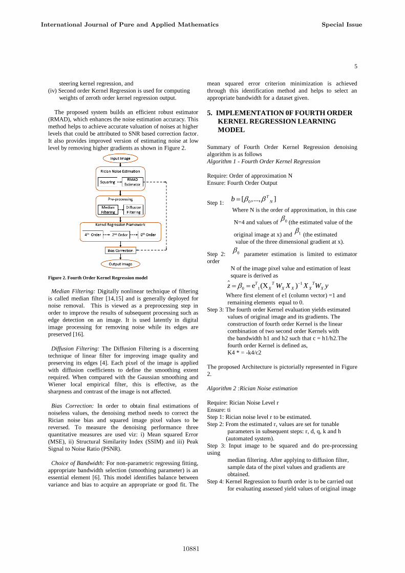
level by removing higher gradients as shown in Figure 2.

Figure 2. Fourth Order Kernel Regression model

Median Filtering: Digitally nonlinear technique of filtering

is called median filter [14,15] and is generally deployed for

noise removal. This is viewed as a preprocessing step in

order to improve the results of subsequent processing such as

edge detection on an image. It is used latently in digital

image processing for removing noise while its edges are

preserved [16].

Diffusion Filtering: The Diffusion Filtering is a discerning

technique of linear filter for improving image quality and

preserving its edges [4]. Each pixel of the image is applied

with diffusion coefficients to define the smoothing extent

required. When compared with the Gaussian smoothing and

Wiener local empirical filter, this is effective, as the

sharpness and contrast of the image is not affected.

Bias Correction: In order to obtain final estimations of

noiseless values, the denoising method needs to correct the

Rician noise bias and squared image pixel values to be

reversed. To measure the denoising performance three

quantitative measures are used viz: i) Mean squared Error

(MSE), ii) Structural Similarity Index (SSIM) and iii) Peak

Signal to Noise Ratio (PSNR).

Choice of Bandwidth: For non-parametric regressing fitting,

appropriate bandwidth selection (smoothing parameter) is an

essential element [6]. This model identifies balance between

variance and bias to acquire an appropriate or good fit. The

mean squared error criterion minimization is achieved

through this identification method and helps to select an

appropriate bandwidth for a dataset given.

5. IMPLEMENTATION 0F FOURTH ORDER

KERNEL REGRESSION LEARNING

MODEL

Summary of Fourth Order Kernel Regression denoising

algorithm is as follows

Algorithm 1 - Fourth Order Kernel Regression

Require: Order of approximation N

Ensure: Fourth Order Output

Step 1: 0[ ,..., ]T

Nb

Where N is the order of approximation, in this case

N=4 and values of 0 (the estimated value of the

original image at x) and 1 (the estimated

value of the three dimensional gradient at x).

Step 2: 0 parameter estimation is limited to estimator

order

N of the image pixel value and estimation of least

square is derived as

1

0 1e (X )T T T

X X X X Xz W X X W y

Where first element of e1 (column vector) =1 and

remaining elements equal to 0.

Step 3: The fourth order Kernel evaluation yields estimated

values of original image and its gradients. The

construction of fourth order Kernel is the linear

combination of two second order Kernels with

the bandwidth h1 and h2 such that c = h1/h2.The

fourth order Kernel is defined as,

K4 * = -k4/c2

The proposed Architecture is pictorially represented in Figure

2.

Algorithm 2 :Rician Noise estimation

Require: Rician Noise Level r

Ensure: ti

Step 1: Rician noise level r to be estimated.

Step 2: From the estimated r, values are set for tunable

parameters in subsequent steps: r, d, q, k and h

(automated system).

Step 3: Input image to be squared and do pre-processing

using

median filtering. After applying to diffusion filter,

sample data of the pixel values and gradients are

obtained.

Step 4: Kernel Regression to fourth order is to be carried out

for evaluating assessed yield values of original image


10881

6

and its gradients subsequently this output is applied

to

second order regression.

Step 5: Kernel regression to second order is applied to obtain

finer readings of pixel values and gradients, b0 and

b1.

Step 6: Obtained results from Step 5 is used to build feature

vectors, and the same is used to perform zeroth order

Kernel regression filtering.

Step 7: Final output ti is obtained by correcting the bias of

zeroth order Kernel regression filtered image and the

estimated noise level r is obtained in Step 1.

6. EXPERIMENTAL RESULT AND ANALYSIS

The experimental results are carried out by using existing

hardware setup and image database. The results for existing

and proposed methods are verified by using MR 3D images

which consists of 181 slices on each image type such as, T1-

weighted, T2-weighted and Pd-weighted images. Denoising

the MR image, smooth regions are filtered by the fourth order

scheme and edges filtered by a second order scheme. During

denoising the MR image, smooth regions are filtered by the

fourth order scheme and edges filtered by a second order

scheme. Sample images are shown in Figure 3.

(a) Brain Web T1 (b) Brain Web T2 (c) Brain Web Pd Figure 3. MRI Brain Image

Database: The Proposed new method has been experimented

using Internet Brain Segmentation Repository (ISBR)

database and gave promising results. Currently there are six

MR brain data sets, which were provided by the Center for

Morphometric Analysis at Massachusetts General Hospital.

Most of them have T1-weighted MR images of healthy

subjects. Two data sets have images of two different patients

with brain tumors. There are three different directories in

which data sets can be found organized into “img”, “seg” and

“otl” directories, which contain the raw, segmented and

outlined images, respectively. However not all data sets have

the “seg” and/or “otl” directories. Raw images are 256x256 of

16-bit, but some of them have also these images scaled to 8-

bit. Segmented images are “trinary” images (pixels are

labeled as a Grey Matter or White Matter tissue or as other),

with the same dimensionality as the raw images[17]. Outlined

images are the outcome of semi- automated segmentation

techniques executed and contain indicators that define certain

structures in each scan image. They are defined in a 512x512

grid, because they were created using over sampled images to

double size. Parameter settings for the pre-computed brain

database are three levels of intensity, non uniformity and

modalities and five levels (1,3,5,7 and 9) of noise. The voxel

values of each image are magnitude in nature and rather

complex, imaginary or real.

MRI T1-weighted: Within the body, the difference of spin

lattice is considered as T1. Subsequently various tissue

relaxation times are referred as T1 weighted. Gradient or spin

echo sequences are used to acquire images of T1 weighted.

Gray and white substances are differentiated by appreciable

contrast as provided by T1-weighted brain scans.

(a) 1% Rician Noise Added (b) Noiseless (c) Restored

(d) 3% Rician Noise Added (e) Noiseless (f) Restored

(g) 5% Rician Noise Added (h) Noiseless (i) Restored

Figure 4. Results for Brain Web T1 weighted synthetic image

MRI T2-weighted: Water is differentiated from fat as lighter

and darker respectively as T2-weighted that is similar to

weighted T1 scan.




10882

7


Figure 5. Results for Brain Web T2 weighted synthetic image.

MRI Pd-weighted: FLAIR sequence could be converted by

weighted sequence of T2 by manipulating magnetic radiance

and added radio frequency pulse. In this sequence free water

and edematous tissues remain dark and bright respectively.




Figure 6. Results for Brain Web Pd weighted synthetic image.

Table 1 shows, that in the existing system maximum PSNR

value achieved is 42.7172. In the proposed method, RMAD

and diffusion filter play an important role in increasing

higher PSNR (43.6481) for noise level (σ = 1) by preserving

edges. RMAD plays another role in the reduction of MSE

from 3.4782 to 2.8072 in the proposed method.

Table 1 : Performance Measures : Existing and proposed

model T1 weighted image of Axial View Test image

/ Method

Noise

added

(in dB)

MSE RMSE PSNR SSIM

Proposed 1 2.8072 1.6755 43.6481 0.9885

Existing 3.4782 1.8650 42.7172 0.9883

Proposed 3 12.0456 3.4707 37.3225 0.9293

Existing 28.8464 5.3709 33.5299 0.8841

Proposed 5 21.8812 4.6776 34.7303 0.8885

Existing 62.9829 7.9362 30.1386 0.8310

Proposed 7 31.6462 5.6255 33.1276 0.8567

85.3016 9.2359 28.8212 0.8130

Proposed 9 45.5723 6.7507 31.5468 0.8411

Existing 253.5114 15.9220 24.0908 0.6433

Table 2 shows for T2-weighted image, the PSNR value is low

for noise level (σ = 1). Higher the noise level (above 1), the

PSNR value is comparably higher than existing method.

Table : 2 Performance Measures for existing and proposed

model for T2-weighted image of Axial View. Test

image/

Method

Noise

added

(in dB)

MSE RMSE PSNR SSIM

Proposed 1 7.1384 2.6718 39.5948 0.9877

Existing 10.6754 3.5643 35.6754 0.9365

Proposed 3 26.5066 5.1485 33.8973 0.9272

Existing 38.2288 6.1829 32.3069 0.9265

Proposed 5 50.5669 7.1110 31.0922 0.8808

Existing 98.1975 9.9095 28.2098 0.8423

Proposed 7 78.962 9.6435 30.0867 0.8563

Existing 164.335 12.8193 25.9735 0.8136

Proposed 9 107.281

8

10.3577 27.8255 0.8270

Existing 351.632

5

18.7519 22.6699 0.7205

In existing system, the maximum PSNR value is achieved

41.9949. In proposed method, RMAD and Diffusion Filter

plays an important role to increase high PSNR (42.2917) for

noise level (σ = 1) by preserving edges. RMAD play another

role to reduce the MSE from 4.8296 to 4.1076 in the proposed

method as shown in Table 3. Resulted images for T1

weighted MRI (Brain Web) are shown in Figure 4.

Table : 3 Performance Measures for existing and proposed

model for Pd-weighted image of Axial View Test

image/Method

Noise

added

(in

dB)

MSE RMSE PSNR SSIM

Proposed 1 4.1076 2.0267 42.2917 0.9860

Existing 4.8296 2.1976 41.9949 0.9833

Proposed 3 15.8563 3.9820 36.1288 0.9373

Existing 35.4161 5.9511 32.6388 0.8849

Proposed 5 28.7566 5.3625 33.5434 0.8983

Existing 91.6619 9.574 28.5089 0.7554

Proposed 7 42.6341 6.5295 31.8332 0.8546

Existing 146.0120 12.0835 26.4869 0.6867

Proposed 9 68.0639 8.2501 29.8016 0.8007

Existing 337.8333 18.3802 22.8438 0.5004

Figure 7 shows the comparison result (RMSE) of the existing

second order kernel regression and the proposed fourth order

kernel regression for T1, T2, Pd weighted images. It clearly

shows that RMSE of the proposed method is lesser than the

existing method. Resulted images for T2 and Pd weighted

MRI (Brain Web) are shown as Figure 5 and 6 respectively.


10883

8

Figure 7. Comparison of RMSE value between Proposed and Existing

method for T1,T2 and Pd Weighted images

Figure 8 shows the comparison result (PSNR) of the existing

second order kernel regression and the proposed fourth order

kernel regression for T1, T2, Pd weighted images. The value

for PSNR is higher than the prevailing method as denoted.

Figure 8. Comparison of PSNR value between Proposed and Existing

method for T1,T2 and Pd Weighted images methods

Figure 9. Comparison of SSIM value between Proposed and Existing

method for T1,T2 and Pd Weighted images

Figure 9 shows the comparison result (SSIM) of the existing

second order kernel regression and proposed fourth order

kernel regression for T1, T2, Pd weighted images. It clearly

shows that the SSIM of the proposed method is greater than

the existing method.

Figure 10. Comparison of Processing Time

Table 4 shows that the processing time of second order

Kernel regression for T1- weighted image is increased when

the noise level increase. For lower noise level, the processing

time is minimal. Considering an example, when the moderate

noise level is 3db, the processing time is 255.81 sec, whereas

in proposed method by combining two second order Kernel

with the bandwidth h1 and h2 linearly so we can achieve the

processing time is 116.50 seconds for noise level 3dB.

Table : 4 Quantitative results for Brain Web T1-weighted

image to calculate processing time (in seconds) for second

order and fourth order Kernel regression.

Test

imag

e

Image

view

Noise

level

added(dB)

Existing-

Second order

Kernel

regression

(in seconds)

Proposed-

Fourth order

Kernel

regression (in

seconds)

1 Axial 1 252.125196 115.94864

2 Axial 3 255.810093 116.50887

3 Axial 5 256.649150 116.74220

4 Axial 7 257.743703 116.940812

5 Axial 9 258.338586 120.585026

Table 5 shows that the processing time of second order

Kernel regression for T2- weighted image is increased when

noise level increases. For lower noise level, the processing

time is minimal. In fourth order Kernel regression for noise

level (σ = 1, 3, 5, 7 and 9) the processing time increases

gradually. For noise level above 9dB the processing time

increases.

Table: 5 Quantitative results for Brain Web T2-weighted


order and fourth order Kernel regression


10884

9

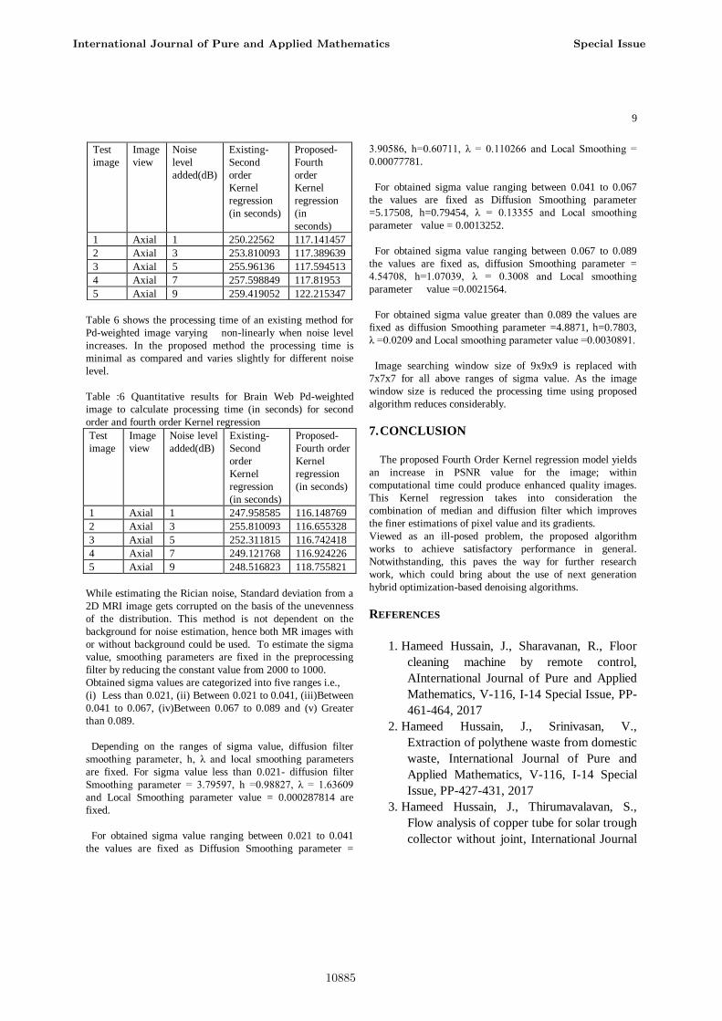
Table 6 shows the processing time of an existing method for

Pd-weighted image varying non-linearly when noise level

increases. In the proposed method the processing time is

minimal as compared and varies slightly for different noise

level.

Table :6 Quantitative results for Brain Web Pd-weighted


order and fourth order Kernel regression

Test

image

Image

view

Noise level

added(dB)

Existing-

Second

order

Kernel

regression

(in seconds)

Proposed-

Fourth order

Kernel

regression

(in seconds)

1 Axial 1 247.958585 116.148769

2 Axial 3 255.810093 116.655328

3 Axial 5 252.311815 116.742418

4 Axial 7 249.121768 116.924226

5 Axial 9 248.516823 118.755821

While estimating the Rician noise, Standard deviation from a

2D MRI image gets corrupted on the basis of the unevenness

of the distribution. This method is not dependent on the

background for noise estimation, hence both MR images with

or without background could be used. To estimate the sigma

value, smoothing parameters are fixed in the preprocessing

filter by reducing the constant value from 2000 to 1000.

Obtained sigma values are categorized into five ranges i.e.,

(i) Less than 0.021, (ii) Between 0.021 to 0.041, (iii)Between

0.041 to 0.067, (iv)Between 0.067 to 0.089 and (v) Greater

than 0.089.

Depending on the ranges of sigma value, diffusion filter

smoothing parameter, h, λ and local smoothing parameters

are fixed. For sigma value less than 0.021- diffusion filter

Smoothing parameter = 3.79597, h =0.98827, λ = 1.63609

and Local Smoothing parameter value = 0.000287814 are

fixed.

For obtained sigma value ranging between 0.021 to 0.041

the values are fixed as Diffusion Smoothing parameter =

3.90586, h=0.60711, λ = 0.110266 and Local Smoothing =

0.00077781.


the values are fixed as Diffusion Smoothing parameter

=5.17508, h=0.79454, λ = 0.13355 and Local smoothing

parameter value = 0.0013252.


the values are fixed as, diffusion Smoothing parameter =

4.54708, h=1.07039, λ = 0.3008 and Local smoothing

parameter value =0.0021564.

For obtained sigma value greater than 0.089 the values are

fixed as diffusion Smoothing parameter =4.8871, h=0.7803,

λ =0.0209 and Local smoothing parameter value =0.0030891.

Image searching window size of 9x9x9 is replaced with

7x7x7 for all above ranges of sigma value. As the image

window size is reduced the processing time using proposed

algorithm reduces considerably.

7. CONCLUSION

The proposed Fourth Order Kernel regression model yields

an increase in PSNR value for the image; within

computational time could produce enhanced quality images.

This Kernel regression takes into consideration the

combination of median and diffusion filter which improves

the finer estimations of pixel value and its gradients.

Viewed as an ill-posed problem, the proposed algorithm

works to achieve satisfactory performance in general.

Notwithstanding, this paves the way for further research

work, which could bring about the use of next generation

hybrid optimization-based denoising algorithms.

REFERENCES

1. Hameed Hussain, J., Sharavanan, R., Floor

cleaning machine by remote control,

AInternational Journal of Pure and Applied

Mathematics, V-116, I-14 Special Issue, PP-

461-464, 2017

2. Hameed Hussain, J., Srinivasan, V.,

Extraction of polythene waste from domestic

waste, International Journal of Pure and

Applied Mathematics, V-116, I-14 Special

Issue, PP-427-431, 2017

3. Hameed Hussain, J., Thirumavalavan, S.,

Flow analysis of copper tube for solar trough

collector without joint, International Journal

Test

image

Image

view

Noise

level

added(dB)

Existing-

Second

order

Kernel

regression

(in seconds)

Proposed-

Fourth

order

Kernel

regression

(in

seconds)

1 Axial 1 250.22562 117.141457

2 Axial 3 253.810093 117.389639

3 Axial 5 255.96136 117.594513

4 Axial 7 257.598849 117.81953

5 Axial 9 259.419052 122.215347


10885

10

of Pure and Applied Mathematics, V-116, I-

14 Special Issue, PP-541-544, 2017

4. Hanirex, D.K., Kaliyamurthie, K.P., Mining

the financial multi-relationship with accurate

models, Middle - East Journal of Scientific

Research, V-19, I-6, PP-795-798, 2014

5. Hemapriya, M., Meikandaan, T.P., Repair of

damaged reinforced concrete beam by

externally bonded with CFRP sheets,

International Journal of Pure and Applied


473-479, 2017

6. Hemapriya, M., Meikandaan, T.P.,

Experimental study on changes in properties

of cement concrete using steel slag and fly

ash, International Journal of Pure and


Issue, PP-369-375, 2017

7. Hemapriya, M., Meikandaan, T.P.,

Experimental study on structural repair and

strengthening of RC beams with FRP

laminates, International Journal of Pure and


Issue, PP-355-361, 2017

8. Hemapriya, M., Meikandaan, T.P., Effect of

high range water reducers on sorptivity and

water permeability of concrete, International

Journal of Pure and Applied Mathematics,

V-116, I-13 Special Issue, PP-377-381,

2017

9. Hemapriya, M., Meikandaan, T.P., Strength

and workability characteristics of super

plasticized concrete, International Journal of

Pure and Applied Mathematics, V-116, I-13

Special Issue, PP-345-353, 2017

10. Hemapriya, M., Meikandaan, T.P., Potency

and workability behavior of quality

plasticized structural material, International


V-116, I-13 Special Issue, PP-363-367,

2017

11. Hussain, J.H., Manavalan, S., Optimization

of properties of jatropha methyl Ester (JME)

from jatropha oil, International Journal of



12. Hussain, J.H., Manavalan, S., Optimization

and comparison of properties of neem and

jatropha biodiesels, International Journal of



13. Hussain, J.H., Meenakshi, C.M., Simulation

and analysis of heavy vehicles composite leaf

spring, International Journal of Pure and


Issue, PP-135-140, 2017

14. Hussain, J.H., Nimal, R.J.G.R., Review:

Investigation on mechanical properties of

different metal matrix composites in diffusion

bonding method by using metal interlayers,



459-464, 2017

15. Jagadeeswari, P., Subashini, G., Basic results

of probability, International Journal of Pure

and Applied Mathematics, V-116, I-17


16. Janani, V.D., Kavitha, S., Conceptual level

similarity measure based review spam

detection adversarial spam detection using

the randomized hough transform-support

vector machine, International Journal of Pure



17. Jasmin, M., Beulah Hemalatha, S., Security

for industrial communication system using

encryption / decryption modules,



563-567, 2017

18. Jasmin, M., Beulah Hemalatha, S., VLSI-

based frequency spectrum analyzer for low

area chip design by using yasmirub method,



557-560, 2017

19. Jasmin, M., Beulah Hemalatha, S., RFID

security and privacy enhancement,



10886

11


535-538, 2017

20. Jasmin, M., Beulah Hemalatha, S., Digital

phase locked loop, International Journal of



21. Jeyalakshmi, G., Arulselvi, S., Community

oriented configurations for WSN,



529-533, 2017

22. Jeyalakshmi, G., Arulselvi, S., Investigating

file systems, International Journal of Pure



23. Jeyalakshmi, G., Arulselvi, S., Methodology

for the development of lambda calculus,



511-515, 2017

24. Jeyalakshmi, G., Arulselvi, S., Remote

procedure calls in access points,



523-526, 2017

25. Jeyanthi Rebecca, L., Anbuselvi, S.,

Sharmila, S., Medok, P., Sarkar, D., Effect

of marine waste on plant growth, Der

Pharmacia Lettre, V-7, I-10, PP-299-301,

2015

26. Kaliyamurthie, K.P., Parameswari, D.,

Udayakumar, R., Malicious packet loss

during routing misbehavior-identification,

Middle - East Journal of Scientific Research,

V-20, I-11, PP-1413-1416, 2014

27. Kanagavalli, G., Sangeetha, M., Intelligent

trafficlight system for reducedfuel

consumption, International Journal of Pure



28. Kanagavalli, G., Sangeetha, M., GPS based

blind pedestrian positioning and voice

response system, International Journal of



29. Kanagavalli, G., Sangeetha, M., Detection of

retinal abnormality by contrast enhancement

methodusing curvelet transform,



497-502, 2017

30. Kanagavalli, G., Sangeetha, M., Design of

low power VLSI circuits for precharge logic,



505-509, 2017

31. Kanniga, E., Selvaramarathnam, K.,

Sundararajan, M., Kandigital bike operating

system, Middle - East Journal of Scientific

Research, V-20, I-6, PP-685-688, 2014

32. Karthik, B., Arulselvi, Noise removal using

mixtures of projected gaussian scale

mixtures, Middle - East Journal of Scientific

Research, V-20, I-12, PP-2335-2340, 2014

33. Karthik, B., Arulselvi, Selvaraj, A., Test data

compression architecture for lowpower vlsi

testing, Middle - East Journal of Scientific

Research, V-20, I-12, PP-2331-2334, 2014

34. Karthikeyan, R., Michael, G., Kumaravel,

A., A housing selection method for design,

implementation&evaluation for web

based recommended systems, International


V-116, I-8 Special Issue, PP-23-27, 2017

35. Khanaa, V., Thooyamani, K.P., Using

lookup table circulating fluidised bed

combustion boiler by the method of sensor

output linearization, Middle - East Journal of

Scientific Research, V-16, I-12, PP-1801-

1806, 2013

36. Khanaa, V., Thooyamani, K.P., Face routing

protocol using genetic algorithm in, Middle -

East Journal of Scientific Research, V-16, I-

12, PP-1863-1867, 2013

37. Khanaa, V., Thooyamani, K.P.,

Udayakumar, R., Two factor authentication

using mobile phones, World Applied

Sciences Journal, V-29, I-14, PP-208-213,

2014


10887

12


Udayakumar, R., Next major wave of it

inovation, World Applied Sciences Journal,

V-29, I-14, PP-218-220, 2014


Udayakumar, R., Traffic policing approach

for wireless video conference traffic, World

Applied Sciences Journal, V-29, I-14, PP-

200-207, 2014


Udayakumar, R., Patient monitoring in gene

ontology with words computing using SOM,

World Applied Sciences Journal, V-29, I-14,

PP-195-199, 2014


Udayakumar, R., Load balancing in

structured PEER to PEER systems, World

Applied Sciences Journal, V-29, I-14, PP-

186-189, 2014


Udayakumar, R., Impact of route stability

under random based mobility model in

MANET, World Applied Sciences Journal,

V-29, I-14, PP-274-278, 2014


Udayakumar, R., Modelling Cloud Storage,

World Applied Sciences Journal, V-29, I-14,

PP-190-194, 2014


Udayakumar, R., Elliptic curve cryptography

using in multicast network, World Applied

Sciences Journal, V-29, I-14, PP-264-269,

2014


Udayakumar, R., SRW/U as a lingua franca

in managing the diversified information

resources, World Applied Sciences Journal,

V-29, I-14, PP-279-284, 2014

.


10888

3D MR Image Denoising Using higher O rder Kernel Regression

Documents

Transcript of 3D MR Image Denoising Using higher O rder Kernel Regression