3D-ICONS- D3 1: Interim Report on Data Acquisition

ICONS

3D ICONS is funded by the European Commission’s ICT Policy Support Programme

D3.1: Interim Report on Data Acquisition

Author:G. Guidi (POLIMI)

3D Digitisation of Icons of European Architectural and Archaeological Heritage

Revision History

Rev. Date Author Org. Description 0.1 11/01/14 G. GUIDI POLIMI First draft 0.2 22/01/14 S.Bassett MDR Editing and review 0.3 29/01/14 G. GUIDI POLIMI Figures and comments 0.4 29/01/14 S.Bassett MDR Editing and review 0.5 30/01/14 F. Nicolucci CISA Editing and review

0.6 31/01/14 G. GUIDI POLIMI Updated final tables after the very last Orpheus data

Revision: [Final] Authors: G. Guidi (POLIMI)

Statement of originality: This deliverable contains original unpublished work except where clearly indicated otherwise. Acknowledgement of previously published material and of the work of others has been made through appropriate citation, quotation or both.

3D-ICONS is a project funded under the European Commission’s ICT Policy Support Programme, project no. 297194.

The views and opinions expressed in this presentation are the sole responsibility of the authors and do not necessarily reflect the views of the European Commission.

iv

Contents

Executive Summary.............................................................................................................................................. 1

1. Introduction ....................................................................................................................................................... 2

2. 3D capturing technologies actually employed for 3DICONS ........................................................... 5

2.1 Passive technologies ................................................................................................................................ 5

2.1.1 Traditional Photogrammetry ....................................................................................................... 7

2.1.2 SFM/Image matching ...................................................................................................................... 7

2.2 Active technologies .................................................................................................................................. 9

2.2.1 Triangulation based range devices ............................................................................................ 9

2.2.2 Direct distance measurement devices based on Time of Flight (TOF) ..................... 11

2.2.3 Direct distance measurement devices based on Phase Shift (PS) .............................. 12

2.3 Relationship between technology and applicative scenarios ............................................... 13

3. Distribution of 3D capturing technologies among the partners ................................................. 15

3.1 ARCHEOTRANFERT .............................................................................................................................. 15

3.2 CETI ............................................................................................................................................................. 15

3.3 CISA ............................................................................................................................................................. 15

3.4 CMC .............................................................................................................................................................. 15

3.5 CNR-ISTI .................................................................................................................................................... 16

3.6 CNR-ITABC................................................................................................................................................ 16

3.7 CYI-STARC ................................................................................................................................................. 16

3.8 DISC ............................................................................................................................................................. 16

v

3.9 FBK .............................................................................................................................................................. 17

3.10 KMKG ....................................................................................................................................................... 17

3.11 MAP-CNRS .............................................................................................................................................. 17

3.12 MNIR ......................................................................................................................................................... 17

3.13 POLIMI ..................................................................................................................................................... 18

3.14 UJA-CAAI ................................................................................................................................................. 18

3.15 VisDim ...................................................................................................................................................... 18

3.16 Considerations about the 3D technologies employed .......................................................... 19

4. State of advancement of WP3 ................................................................................................................... 22

Appendix - Detailed state of digitization by unit ................................................................................... 26

1

Executive Summary Deliverable 3.1 Interim Report on Data Acquisition is a preliminary overview of all the

activities related with digitization (WP3), at month 17 of the 24 allocated for WP3 (M6

to M30). This interim report shows how the WP3 activity is proceeding, both globally

and at partner level, proving also feedback to the project management for deciding

possible corrective actions.

The information for this report was taken from the Progress Monitoring Tool and a

short WP3 survey questionnaire completed by all the content providers. The analysis of

the questionnaire responses show that a wide range of data acquisition technologies are

being used with the most popular one being photogrammetry (used by thirteen

partners). Laser scanning for large volumes is also widely used (nine partners), whilst

only five are using small volume laser scanning. Only two partners produce 3D content

with CAD modelling, starting from pre-existing documentation/surveys. An overview of

both the passive and active scanning technologies is provided to aid the understanding

of the current work being undertaken in WP3 of 3D-ICONS.

Regarding the progress of WP3, the global situation shows that, although some delays

have influenced the activity of a few partners, the project is properly proceeding, having

completed the 62% of the digitization work. Actually, 17/24 corresponds approximately

to 71%, which would be the amount of work done to be perfectly on time. But we have

to consider that in the initial phase of WP3, some of the partners – especially those less

technically skilled or experienced with 3D modelling- needed a few months for setting

up the most optimized 3D acquisition strategy, tailored to the work each partner is

expected to carry out in the WP3 period.

Considering, therefore, from 2 to 5 months initial phase at zero or low productivity due

to the start-up of this unprecedented massive 3D acquisition activity, we can see that

the operating months at full rate are about 12 to 15, which compared with the duration

of the Work Package gives and average of 62%, as actually performed by the project.

Furthermore, considering the last semester, digitization activity appears to have been

significantly accelerated by each unit, so the achievement of the targets by M30 seems

definitely feasible.

However, if necessary, with six months left beyond M30, small delays in digitization can

be absorbed into the remaining schedule without affecting the final delivery of models

and metadata at M36.

2

D3.1 Interim report on data acquisition

1. Introduction The digitization action expected as output of WP3 is referred to the collection of the

three-dimensional data needed for creating, in the framework of WP4, the 3D models

that will be then converted in a form suitable for publication (WP5), enriched with both

technical and descriptive metadata (WP4), structured as defined in WP6. The 3D

models will also be loaded in a project repository, whose creation has been recently

started. This repository will allow each partner to store their 3D content and define a

Uniform Resource Locator (URL) to be associated with the model. Such a URL, included

in the metadata record to be uploaded into EUROPEANA, will allow users to connect the

data records accessible through the EUROPEANA portal to the actual 3D content or a

simplified representation of it, as shown by the block diagram in Figure 1.

The 3D-ICONS project involves two complementary “channels” for collecting 3D data.

Figure 1 - Synthetic representation of the whole data collection involved in the 3D-Icons project. The activity

of WP3 are part of those involved in the “3D capture” block. The metadata record and an iconic

representation of the model (thumbnail image) are ingested into EUROPEANA.

3

On the one hand, the project takes account of a set of pre-existing 3D models of

significant Cultural Heritage assets originated by both 3D acquisition and CAD modeling

in the framework of previous works/projects whose purposes were different from the

generation of 3D content for EUROPEANA. In this way, a patrimony of data, otherwise

unused, acquired over the years by some of the project partners, can usefully be put at

the disposal of the community. The WP3 activity in this case consists in properly

checking and converting datasets already existing, in order to have them available for

the project.

Finally the project pursues the 3D acquisition of new Cultural Heritage assets that will

allow, at the end of the ingestion process planned in the 3DICONS pipeline, to add about

3,000 new 3D items to EUROPEANA.

The main tool that has been used for evaluating the WP3 state of advancement is the

Database developed by the CETI unit (http://orpheus.ceti.gr/3d_icons/), available to

project partners and the EU commission for checking the progress of the whole project,

also by comparing the actual target objectives with what is expected from the project

DOW. This was complemented by an on-line questionnaire

(https://docs.google.com/forms/d/1ciBxCs3ygbYldTUeyVNlP_9Z5G-y_Dj7FE0EBVUC0Co/viewform)

that allowed these figures to be integrated with complementary information related to

the 3D technologies employed by the various partners for carrying out the digitization

phase.

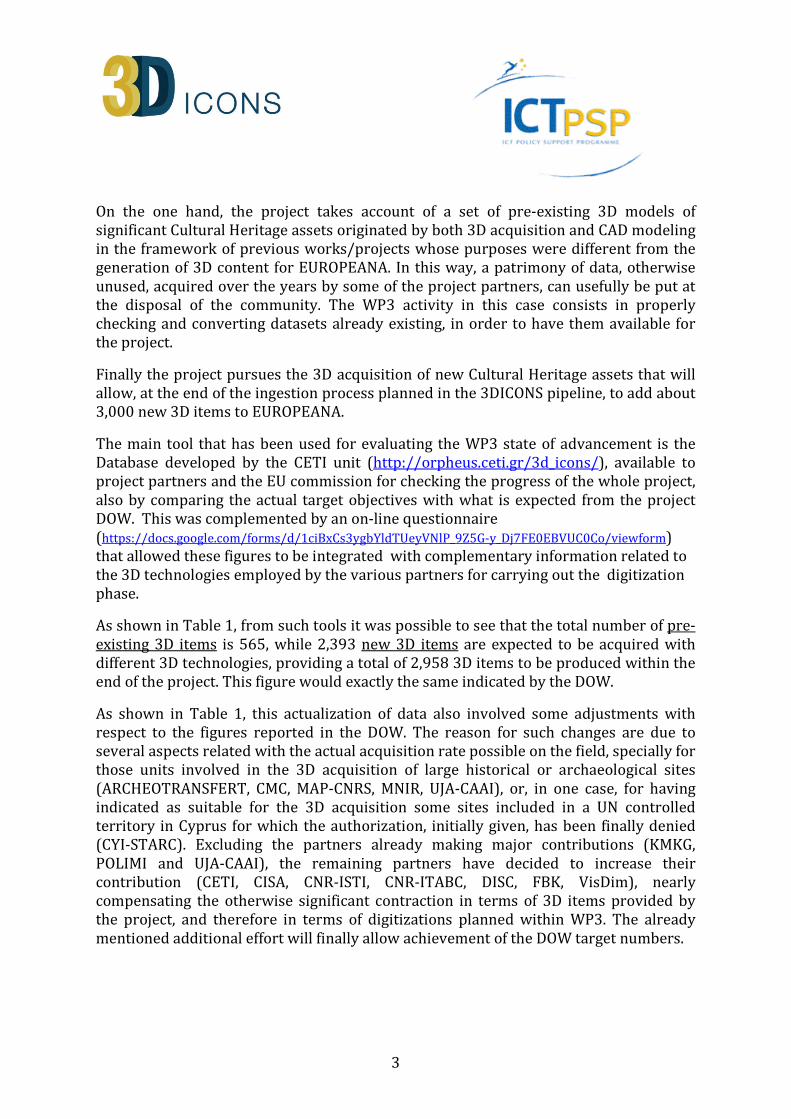
As shown in Table 1, from such tools it was possible to see that the total number of pre-

existing 3D items is 565, while 2,393 new 3D items are expected to be acquired with

different 3D technologies, providing a total of 2,958 3D items to be produced within the

end of the project. This figure would exactly the same indicated by the DOW.

As shown in Table 1, this actualization of data also involved some adjustments with

respect to the figures reported in the DOW. The reason for such changes are due to

several aspects related with the actual acquisition rate possible on the field, specially for

those units involved in the 3D acquisition of large historical or archaeological sites

(ARCHEOTRANSFERT, CMC, MAP-CNRS, MNIR, UJA-CAAI), or, in one case, for having

indicated as suitable for the 3D acquisition some sites included in a UN controlled

territory in Cyprus for which the authorization, initially given, has been finally denied

(CYI-STARC). Excluding the partners already making major contributions (KMKG,

POLIMI and UJA-CAAI), the remaining partners have decided to increase their

contribution (CETI, CISA, CNR-ISTI, CNR-ITABC, DISC, FBK, VisDim), nearly

compensating the otherwise significant contraction in terms of 3D items provided by

the project, and therefore in terms of digitizations planned within WP3. The already

mentioned additional effort will finally allow achievement of the DOW target numbers.

4

Partner Number of 3D

models declared in DOW

Change respect to DOW

Number of 3D models declared in the Orpheus DB

Of which

+ - Pre-

existing New

ARCHEOTR. 258 54 204 62 142

CETI 30 6 36 0 36

CISA 33 50 83 50 33

CMC 53 33 20 0 20

CNR-ISTI 42 143 185 81 104

CNR-ITABC 143 11 154 92 62

CYI-STARC 71 30 41 20 21

DISC 85 24 109 4 105

FBK 57 2 59 13 46

KMKG 450 5 455 0 455

MAP-CNRS 366 17 349 133 216

MNIR 80 20 100 0 100

POLIMI 527 527 55 472

UJA-CAAI 763 177 586 5 581

VisDim 0 50 50 50 0

Total 2958 0 2958 565 2393

Table 1 – Overview of the numbers of digitizations expected by partner, as specified in the DOW in the

planning phase and as actualized in a more advanced phase of the project, evidencing pre-existing and new

3D models.

5

2. 3D capturing technologies actually employed for 3DICONS The technologies actually employed in the framework of the WP3 lie in the taxonomy

already shown in D 2.1, section 7, where a first broad distinction has been made

between technologies based on passive or active measurement methods. Both

principles fall in the category of non-contact measurement methods, very appropriate

for Cultural Heritage objects, being generally delicate and not always suitable to be

touched.

The absence of contact between the measurement device and Cultural Heritage artifact

is obtained because the probing element, instead of a physical tip touching the surface

to be measured for collecting its 3D coordinates at the contact point (as, for example, in

the so-called Coordinate Measurement Machines or CMMs), is a beam of radiating

energy projected onto the surface to be probed. This beam interacts with the surface

and is deflected and measured by the scanning device, enabling the relative position of

the current scanned point to be calculated. In this way, a complete set of co-ordinates or

“point cloud” is built up which detects the geometrical structure of the scanned object.

When the form of energy employed is light (including non-visible radiation like Infra

Red), we talk of optical 3D methods, where the main difference between active and

passive lies in the way such light is provided.

2.1 Passive technologies

In a passive device, light is used just for making clear the details of the scene. These

details have to be clearly visible elements contrasting with the background and richly

present on all the points of the surface of interest for capture. This is a characteristic,

for example, of photogrammetry, a typical passive method based on multiple images of

the same scene, taken from different positions. Here the measurement process requires,

first of all, to recognize the same points in different shots of a scene, and this is possible

only if the measured object is provided with a contrasted texture, or - when the object is

uniformly colored with no salient points - if the operator has added a reference target

over the surface of interest in a number of points sufficient for estimating its 3D shape.

The typical pipeline for creating a 3D model with photogrammetric methods involves

the following steps:

1. Calibration – The camera distortions (radial, tangential and affine) are

estimated through a proper calibration procedure. If the camera has

interchangeable lenses like a reflex or a last generation mirrorless camera, each

camera-lens combination needs to be calibrated.

2. Image acquisition – A suitable set of images of the object to be surveyed are

taken with the same setting that has been calibrated, considering that for

collecting the 3D information of a point at least two images must contain that

point. The number of images needed to carry out the complete 3D measurement

6

of a CH object is highly influenced by its size, the resolution needed, and the way

resection, the next step, is implemented.

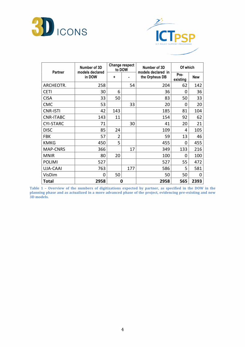
3. Resection - This phase calculates the orientation in the 3D space of the camera

while taking the images acquired in the step 2. The means for estimating such

orientation is identifying a suitable number of correspondence points in

adjacent images using their coordinates as input to a non-linear optimization

process (bundle adjustment), minimizing the re-projection error on the actual

image points of their corresponding 3D estimates. In traditional

photogrammetry, this phase is quite lengthy because, unless coded targets are

used, the identification of correspondences is a manual operation. In the last few

years a more modern approach has been developed, allowing automatically

identification of correspondence points by analyzing the image content

(Structure From Motion or SFM). This requires that adjacent images cannot

differ too much, so the level of superposition of such shots has to be high (at least

60%), and consequently the number of shots to be taken is much higher than in

traditional photogrammetry. However, the need to find correspondences

generally discourages the use of passive methods for objects with little or no

texture.

4. Intersection – This phase calculates the 3D coordinates of corresponding points

by the intersection of two rays associated with the same point seen on two

different images (triangulation). Also, in this case, the process can be extremely

time consuming if the end-user has to manually identify the points of interest,

generating in this way a specific selection of 3D points taken in suitable positions

(sparse 3D cloud). A more modern process implemented in recent years, and

usually associated with SFM, is the so-called “dense image matching”, that –

given a certain orientation - automatically finds a regular set of correspondences

between two or more images, thereby calculating a dense cloud of evenly spaced

3D points. The interesting aspect of this approach is that each group of 3D points,

is “naturally” oriented in a single coordinate system;

5. Scaling – The cloud of 3D points generated by steps 1-4 is a relative estimation

of coordinates. There is no metric correspondence with the physical reality they

are representing. In order to obtain a set of metric 3D points, one or more

reference measurements from the scene have to be provided and the 3D points

have to be scaled accordingly;

6. Modeling – This phase involves the generation of the 3D model starting from the

measured points. Again, its implementation can be done manually on sparse 3D

clouds, or automatically on dense cloud of 3D points. In this latter case, a

topological revision and an editing phase is usually needed.

7

The quality of the result – like for photography - greatly depends on the optical quality

of the equipment used. Good digital reflex cameras with high quality lenses, used by

skilled operators, provide the best image quality for the following 3D processing.

The two implementations of this method used in 3D-CONS are as follows.

2.1.1 Traditional Photogrammetry

All the 6 steps listed previously for the photogrammetric pipeline are done separately

by an operator that has to: a) calibrate the camera by photographing a specific certified

target (e.g. a 3D grid of some tens of known points) and processing the images with a

software capable of providing the distortion parameters from them; b) take photos of

the subject, taking into consideration a proper distance between shots in order to have

a large base for triangulation (the rule of the thumb is to use a distance between

shooting positions approximately equal to 1/3 of the camera-target distance); c) orient

all images in the set identifying a suitable number of correspondence points (at least 8-

10) for each of the images involved, finally applying bundle adjustment; d) identify

some points of the object needed for reconstructing its shape over the oriented images,

and collect their 3D coordinates; e) scale the obtained 3D data set and export to 3D

modeling software; f) draw a 3D model over the measured 3D points.

This method is implemented in both open source and commercial photogrammetry

software packages. It is rather fairly but the associated process is quite cumbersome

and needs a considerable amount of time and skilled operators. The required time is

further increased if the object has no salient reference points and its surface need to be

prepared with specific targets attached to it (not always possible on Cultural Heritage

assets).

2.1.2 SFM/Image matching

This process has been greatly developed in the last ten years and is now a standard

operating tool. It implements the six step photogrammetric pipeline using a high level of

automation, reducing significantly the time needed for generating a 3D model from a set

of images. It is based on the automatic identification of image elements in photographs,

possible if the images have a short base of triangulation (i.e. they are very similar each

other). The process can be implemented through an on-line service (Autodesk 123D

Catch, Microsoft Photosynth, etc.) taking as input a set of images and providing as

output a texturized 3D model, with no user control.

8

a) b)

Figure 2 – SFM digitization made by the POLIMI unit of a Roman altar conserved at the Archaeological

Museum of Milan through AGISOFT Photoscan: a) images automatically oriented in 3D; b) rendering of the 3D

model originated by this method.

But within the 3DICONS project an alternative commercial solution has been widely

adopted by many of the partners (AGISOFT Photoscan). Although this works in a similar

way, it is a piece of software installed locally by the end-user that allows a certain level

of user control over the process.

The operator only needs: a) to acquire a number of images all around the object with a

sufficient overlap (suggested 60%) between adjacent shots as indicated in step 2; b)

launch the process that automatically identifies many (in the order of some thousands)

corresponding points and automatically performs the steps 1 and 3 of the

photogrammetric pipeline, generating a first quality feedback about image orientations;

c) if the orientations are acceptable, a second process can be launched, performing steps

4 and 6 of the photogrammetric pipeline. The set of points obtained is a dense cloud of

3D points including colour information that the software can mesh automatically. The

last point (step 5.) has to be done afterwards in order to provide a metric 3D model. The

result obtained at this step – with the exception of a few editing operations – represents

the final 3D result (Figure 2).

This method produces particularly effective results and has been used by many of the

3DICONS project partners, as shown in detail in section 3.

9

2.2 Active technologies

In an active device, light is not uniformly distributed like a passive device, but is coded

in such a way to contribute to the 3D measurement process. The light used for this

purpose might be both white, as a pattern of light generated with a common LCD

projector, or single wavelength as in a laser. Active systems, particularly those based on

laser light, make the measurement result almost independent of the texture of the

object being photographed, projecting references onto its surface through a suitably

coded light. Such light is characterized by an intrinsic information content recognizable

by an electronic sensor, unlike the environmental diffuse light, which has no

particularly identifiable elements. For example, an array of dots or a series of coloured

bands are all forms of coded light. Thanks to such coding, active 3D sensors can acquire

in digital form the spatial behavior of an object surface. At present, 3D active methods

are quite popular because they are the only ones capable of metrically acquiring the

geometry of a surface in a totally automatic way, with no need to resize according to one

or more given measurements taken from the field. In the 3D-ICONS project such devices

have been largely used in the different implementations described in the following

sections.

2.2.1 Triangulation based range devices

For measuring small volumes, indicatively below a cubic meter, scanners are based on

the principle of triangulation. Exceptional use of these devices have been made in

Cultural Heritage (CH) applications on large artifacts like, for example, the Portalada 3D

scanning performed within this project by the CNR-ISTI unit. In such cases, these are

typically integrated with other types of devices.

The kind of light that was first used to create a 3D scanner is the laser light. Due to its

physical properties, it allows generation of extremely focused spots at relatively long

ranges from the light source, relative to what can be done, for example, with a halogen

lamp. The reason for this is related to the intimate structure of light, which is made by

photons, short packets of electromagnetic energy characterized by their own

wavelength and phase. Lasers generate light which is monochromatic (i.e. consisting of

photons all at the same wavelength), and coherent (i.e. such that all its photons are

generated in different time instants but with the same phase). The practical

consequence of mono-chromaticity is that the lenses used for focusing a laser can be

much more effective, being designed for a single wavelength rather than the wide

spectrum of wavelengths typical of white light. In other words, with a laser it is easier to

concentrate energy in space. On the other hand, the second property of coherence

allows all the photons to generate a constructive wave interference whose consequence

is a concentration of energy in time. Both these factors contribute to making the laser an

effective illumination source for selecting specific points of a scene with high contrast

respect to the background, allowing measurement of their spatial positions as

described below.

10

Figure 3 – Block diagram of a range measurement device based on triangulation: a) a laser beam inclined

with angle α respect to the reference system, impinging on the surface to be measured. The light source is at

distance b from the optical center of a camera equipped with a lens with focal length f. Evaluating the

parallax p from the captured image it is possible to evaluate ββββ; b) combining αααα and b (known for calibration)

and ββββ, the distance ZA can be easily evaluated as the height of this triangle.

A triangulation 3D sensor is a range device made by the composition of a light source

and a planar sensor, rigidly bounded to each other. In the example of Figure 3, the laser

source generates a thin ray producing a small light dot on the surface to be measured. If

we put a digital camera displaced with respect to the light source and the surface is

diffusive enough to reflect some light also towards the camera pupil, an image

containing the light spot can be picked up. In this opto-geometric set-up, the light

source emitting aperture, the projection centre and light spot on the object, form a

triangle as the one shown in Fig. 3b, where the distance between the image capturing

device and light source is indicated as baseline b. In such conditions, the sensor-to-

object distance (ZA) can be easily evaluated, and from this the other value XA calculated.

The principle described above can be extended by a single point of light to a set of

aligned points forming a segment. Systems of this kind use a sheet of light generated by

a laser reflected by a rotating mirror or a cylindrical lens. Once projected onto a flat

surface, such a light plane produces a straight line which becomes a curved profile on

complex surfaces. Each profile point responds to the rule already seen for the single

spot system, with the only difference being that the sensor has to be 2D, so that both

horizontal and vertical parallaxes can be estimated for each profile point. These

parallaxes are used for estimating the corresponding horizontal and vertical angles,

from which, together with the knowledge on the baseline b and the optical focal length f,

the three coordinates of each profile point can be calculated with a high degree of

accuracy. This process therefore allows to the calculation of an array of 3D coordinates

corresponding to the illuminated profile for a given light-object relative positioning. The

described set of the laser sheet generator and camera represent the scanner head. By

11

moving the sheet of light according to a rotational or translation geometry, the whole

set of 3D profiles collected represent a 3D view of the scene.

A similar result is obtained if, instead of moving a single profile over the surface, several

profiles are projected at once. This is in the method used by pattern projection sensors,

where multiple sheets of light are simultaneously produced by a special projector

generating halogen light patterns of horizontal or vertical black and white stripes. An

image of the area illuminated by the pattern is captured with a digital camera and each

Black-to-White (B-W) transition is used as geometrical profile, similar to those

produced by a sheet of laser light impinging on an unknown surface. Even if the

triangulating principle used is exactly the same as for the two laser devices, the main

difference is that here no moving parts are required since no actual scan action is

performed. The range map is computed through digital post-processing of the acquired

image.

The output attainable from both kind of triangulation devices can be seen as an image

having in each pixel the spatial coordinates (x, y, z) expressed in millimeters, optionally

enriched with color information (R, G, B) or by the laser reflectance (Y). This set of 3D

data, called “range image” or “range map”, is generally a 2.5D entity (i.e. at each couple

of x, y values, only one z is defined).

In metrological terms these kind of devices provide low uncertainty (below 0.1 mm),

but can only work in a limited range of distances, generally between 0.5 to 2 metres. So

they are very suitable for small objects with little or no texture, and not too shiny or

transparent.

2.2.2 Direct distance measurement devices based on Time of Flight (TOF)

With active range sensing methods based on triangulation, the size of volumes that can

be easily acquired ranges from a shoe box to a full size statue. For a precise sensor

response, the ratio between camera-target distance and camera-source distance

(baseline), has to be maintained between 1 and 5. Therefore, framing areas very far

from the camera would involve a very large baseline, that above 1m becomes difficult to

be practically implemented. For larger objects like buildings, bridges or castles, a

different working principle is used. It is based on optically measuring the sensor-to-

target distance, having the a priori knowledge of angles through the controlled

orientation of the range measurement device.

TOF range sensing is logically derived from the so-called “total station”. This is made by

a theodolite, namely an optical targeting device for aiming at a specific point in space,

coupled with a goniometer for precisely measuring horizontal and vertical orientations,

integrated with an electronic distance meter. TOF, or time of flight, refers to the method

used for estimating the sensor-to-target distance that is usually done by measuring the

time needed by a pulse of light for travelling from the light source to the target surface

and back to the light detector integrated in the electronic distance meter.

12

A 3D laser scanner is different from a total station in that it does not need a human

operator to aim at a specific point in space and therefore it does not have such a

sophisticate crosshair. On the other hand, it has the capability to automatically re-orient

the laser on a predefined range of horizontal and vertical angles with an assigned

angular resolution, in order to select a specific area in front of the instrument. The

precise angular estimations are then returned by a set of digital encoders, while the

laser TOF gives the distance. By combining this information representing the polar

representation of each point coordinate, the corresponding Cartesian coordinates can

be easily calculated.

For ground-based range sensors, the angular movement can be 360° horizontally and

close to 150° vertically, with an operating range from less that one meter to several

hundred meters or more (depending on the actual implementation), allowing a huge

spherical volume to be captured from a fixed position. As for triangulation based range

sensors, the output of such devices is again a cloud of 3D points originated by a high

resolution spatial sampling of an object. The difference with triangulation devices is

often in the data structure. In TOF devices, data is collected by sampling an angular

sector of a sphere, with a step that is not always fixed. As a result, the data set can be

formed by scan lines that are not necessarily all of the same size. Therefore, the device

output may be a simple list of 3D coordinates not structured in a matrix.

In term of performances, contributions to measurement errors may be made by both

angular estimation accuracy and distance measurements. However, due to the very high

speed of light, the TOF is very short, and this means that the major source of

randomness is due to its estimation that becomes a geometrical uncertainty once time is

converted in distance. Generally, a strength of this kind of device is that the only

distance limiting factor is the laser power, so that the principle can be used also for very

long range devices, like those used in Airborne Laser Scanning (ALS), capable of

collecting 3D data from thousands of metres.

2.2.3 Direct distance measurement devices based on Phase Shift (PS)

In this technique distance is estimated with a laser light whose intensity is sinusoidally

modulated at a known frequency, generating a continuous wave of light energy directed

toward the target. The backscattering on the target surface returns a sinusoidal light

wave delayed with respect to the transmitted one, and therefore characterized by a

phase difference from it.

Since the phase is directly proportional to the distance, from this value the range can be

evaluated similarly as in the previous case. This indirect estimation of distance allows a

better performance in term of uncertainty for two main reasons: a) since the light sent

to the target is continuous, much more energy can be transmitted respect to the TOF

case, and the consequent signal-to-noise ratio of the received signal is higher; b) the

low-pass filtering required for extracting the useful signal component involves an

attenuation of the high frequency noise, resulting in a further decrease of noise with

respect to signal.

13

A peculiar aspect of this range measurement technique is the possibility of ambiguous

information if the sensor-to-target distance is longer than the equivalent length of a full

wave of modulated light, given by the ambiguity range ramb=πc/ω0, due to the periodical

repetition of phase. Such ambiguity involves a maximum operating distance that is in

general smaller for PS devices rather than TOF. For this reason PS are generally used for

medium range operating distances, while TOF are used for long range.

However, the scanning mechanism remains the same as TOF devices, allowing an

horizontal angular scan of 360° and a vertical one around 150°, covering almost a whole

spherical view.

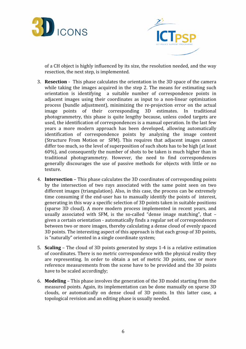
2.3 Relationship between technology and applicative scenarios

The different working principles allow implementation of 3D capturing solutions for

various applicative situations. Figure 4 provides an overview of the device-to-target

distance that is implicitly related to the device’s field of view.

As shown in Figure 4, the low range devices are those based on triangulation, like laser

scanners based on a sheet of light (e.g. Minolta Vivid 910), or on pattern projection (e.g.

Breuckmann Smartscan HE). All these are generally used on a tripod and require a

significant post-processing effort for aligning the various range maps required to cover

the whole surface of an object. As an alternative for fast 3D capture, recent

triangulation-based devices offer on-the-flight evaluation of their position and

orientation with respect to the scene. Therefore, they can be handheld and used more

easily for fairly larger scanning volumes (e.g. Artec EVA; Z-Corp Z-Scanner 800).

Consequently, these are commonly used for small archaeological artifacts, object

museums, etc.

For medium range applications, PS laser scanners work well for interiors or

small/medium architectural structures and archaeological sites. Their speed, in the

range of 1 million of points per second, allows them to be used in complex structures

where several scanner positioning are needed.

For long range applications, TOF laser scanners are the most suitable. Even if usually

slower that PS devices, they can be used as terrestrial devices, in the same way as PS

laser scanners, for capturing large structures or even natural landmarks (e.g. the FBK

unit used this device for capturing a famous rocky mountain in the Dolomites). But since

they have no intrinsic range limitations, they can also be mounted on flying vehicles for

capturing large sites from above with the so-called Airborne Laser Scanner (ALS).

Finally Photogrammetry, both in its traditional implementation and in the more recent

SFM/image matching version, covers the widest range of applicative situations. In

principle, there are no intrinsic range limitations. The only parameter to be taken into

account is the required resolution (or GSD – Ground Sampling Distance), which is

influenced by the lens used (wide-angular vs. teleobjective), and by the camera-to-

14

target distance. This flexibility probably explains why this method is the most widely

used among the 3DICONS partners, as shown in section 3.

Figure 4 – Field of applicability of the various 3D technologies used in the 3DICONS project. The upper limit of

1000 meters is just indicative of a long range, since TOF LS and Photogrammetry can work even from longer

distances.

15

3. Distribution of 3D capturing technologies among the partners According to the questionnaire completed by the partners, a survey about the 3D

technologies employed by the various partners has been conducted, revealing a

diffusion of many different approaches, with a predominance of SFM/Photogrammetry

for its ease of use and speed. All the partners answered the questionnaire, showing an

interesting coverage of the whole 3D digitization area. The results are reported as

follows.

3.1 ARCHEOTRANFERT

Which 3D acquisition technology have you used in WP3?

SFM/Photogrammetry (dense 3D cloud), Traditional photogrammetry (sparse

3D cloud)

Which of them you used more?

SFM/Photogrammetry (dense 3D cloud)

Which Camera/Lens did you use?

Nikon D800E

3.2 CETI


SFM/Photogrammetry (dense 3D cloud), TOF/PS laser scanner




DSLR Nikon D40 at 6.1MP with an 18–55 mm lens; Canon EOS350d at 8.1MP

with an 18–55 mm lens; Samsung NX1000 at 20MP with an 20-50 mm; Nikon

D320 at 24MP with an 10-20mm

Which range sensing which devices did you use?

Optec Ilris 36D

3.3 CISA


SFM/Photogrammetry (dense 3D cloud), TOF/PS laser scanner, CAD Modeling


We use a bit of everything


Nikon D90/ 18-55 mm


Zoller & Froilich Imager 5003

3.4 CMC


TOF/PS laser scanner


We are using data acquired by 3rd parties, who primarily used Leica hardware.

16

3.5 CNR-ISTI


SFM/Photogrammetry (dense 3D cloud), Triangulation range sensor, TOF/PS

laser scanner


Triangulation range sensors


Nikon D 5200, Nikon D70, various compact cameras


long range: Leica Scan Station / Leica 2500 / Leica 3000, RIEGL LMS-Z, FARO

Photon 120

triangulation: Minolta Vivid Vi 910, Breuckman Smartscan-HE, NextEngine

Desktop Scanner"

3.6 CNR-ITABC


SFM/Photogrammetry (dense 3D cloud), TOF/PS laser scanner


SFM/Photogrammetry


Canon 60D 17mm; Canon 650D 18-50 mm; Nikon D200 (fullframe) 15mm


Faro focus 3D

Other technologies?

Spherical Photogrammetry (Canon 60D 17 mm)

3.7 CYI-STARC



3D cloud)



3.8 DISC



laser scanner, Airborne Laser Scanner (ALS)


TOF/PS Laser scanners


Canon 5D MK II/ 24mm - 105mm/ 20mm


Faro Focus 3D, Fli MAP-400 ALS, Artec EVA

17

3.9 FBK



3D cloud), Triangulation range sensor, TOF/PS laser scanner


SFM/Photogrammetry


Nikon D3X/ 50mm; Nikon D3100/ 18 mm; Nikon D3100/ 35mm


Leica HDS7000; ShapeGrabber SG101: Leica ScanStation2; FARO Focus3D

3.10 KMKG




Canon, different cameras and lenses

3.11 MAP-CNRS



3D cloud), Triangulation range sensor, TOF/PS laser scanner




Nikon D1x, D2x and D3x with 20mm, 35mm, 50mm, 105mm, 180mm


Faro Focus 3D, Faro Photon 80, Konica Minolta Vivid 910, Trimble Gx, Mensi

GS200

3.12 MNIR



3D cloud)


SFM/Photogrammetry


Canon EOS 40D, 17-40mm; Nikon D3100, 18-105mm

18

3.13 POLIMI



laser scanner


SFM/Photogrammetry


Canon 5D Mark II/20 mm and 50 mm; Canon 60D/20 mm, 50 mm and 60 mm;

Canon 20D/ 20 mm; Sony Nex-6/Zeiss 24 mm


Minolta Vivid 910; Faro Focus 3D; Leica HDS3100

3.14 UJA-CAAI



3D cloud), Self positioning handheld 3D scanner


SFM/Photogrammetry


Canon EOS 40D/SIGMA DC 18-200mm and EOS APO MACRO 350mm


Z-Scanner 800

3.15 VisDim


Virtual Reconstruction

Other technologies?

3D virtual reconstruction based upon archaeological plans, publications,

measurements and observations on site, interpretation by experts.

The 3D models were built in ArchCAD, improved and retextured in Blender. The

terrain and vegetation is done in Vue.

19

3.16 Considerations about the 3D technologies employed

A wide range of technologies are used within the project due to the type of objects to be

digitized which range from entire archeological sites to buildings, sculptures and

smaller museum artifacts as shown in Table 2.

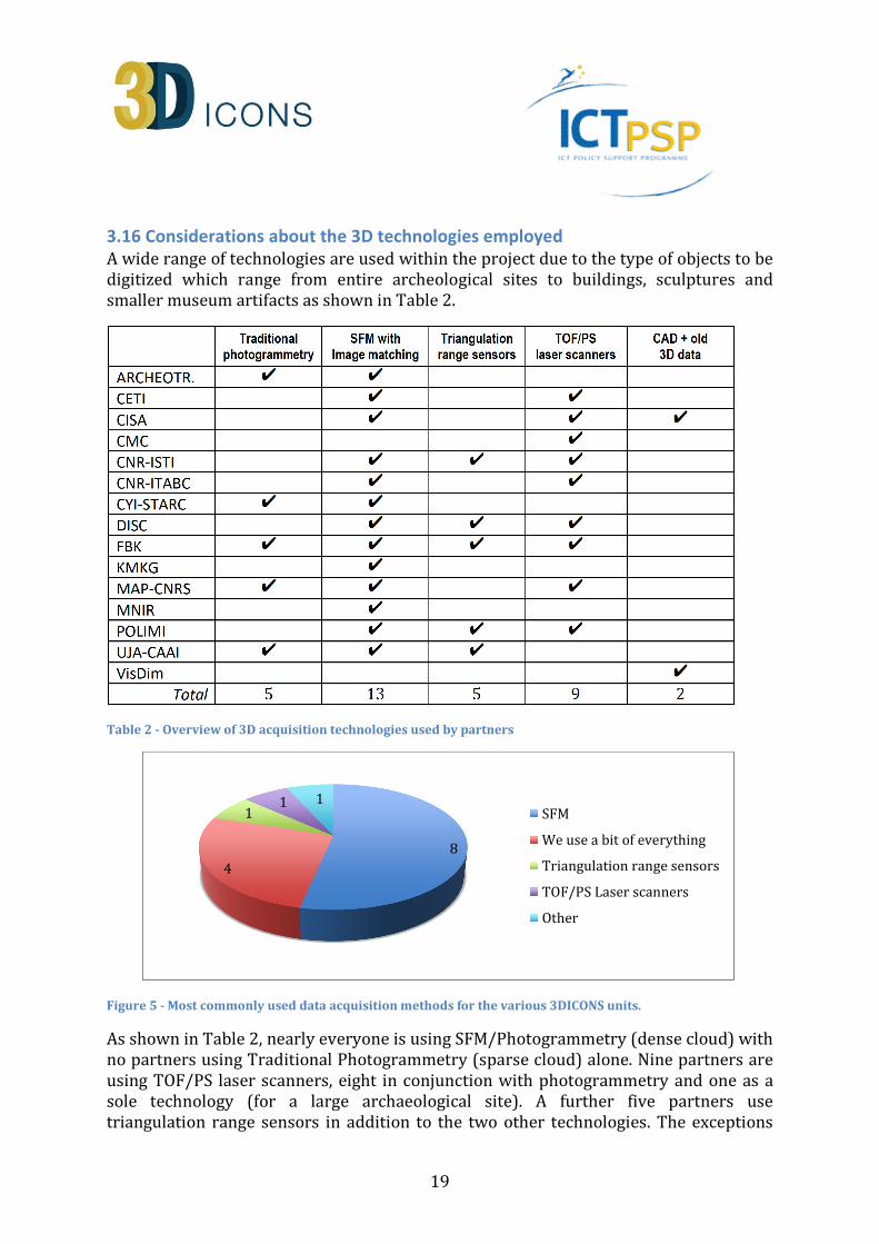
Table 2 - Overview of 3D acquisition technologies used by partners

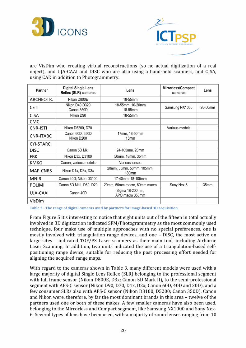
Figure 5 - Most commonly used data acquisition methods for the various 3DICONS units.

As shown in Table 2, nearly everyone is using SFM/Photogrammetry (dense cloud) with

no partners using Traditional Photogrammetry (sparse cloud) alone. Nine partners are

using TOF/PS laser scanners, eight in conjunction with photogrammetry and one as a

sole technology (for a large archaeological site). A further five partners use

triangulation range sensors in addition to the two other technologies. The exceptions

8

4

11 1

SFM


Triangulation range sensors

TOF/PS Laser scanners

Other

20

are VisDim who creating virtual reconstructions (so no actual digitization of a real

object), and UJA-CAAI and DISC who are also using a hand-held scanners, and CISA,

using CAD in addition to Photogrammetry.

Partner Digital Single Lens

Reflex (SLR) cameras Lens

Mirrorless/Compact cameras

Lens

ARCHEOTR. Nikon D800E 18-55mm

CETI Nikon D40,D320

Canon 350D 18-55mm, 10-20mm

18-55mm Samsung NX1000 20-50mm

CISA Nikon D90 18-55mm

CMC

CNR-ISTI Nikon D5200, D70 Various models

CNR-ITABC Canon 60D, 650D

Nikon D200 17mm, 18-50mm

15mm

CYI-STARC

DISC Canon 5D MkII 24-105mm, 20mm

FBK Nikon D3x, D3100 50mm, 18mm, 35mm

KMKG Canon, various models Various lenses

MAP-CNRS Nikon D1x, D2x, D3x 20mm, 35mm, 50mm, 105mm,

180mm

MNIR Canon 40D; Nikon D3100 17-40mm; 18-105mm

POLIMI Canon 5D MkII, D60, D20 20mm, 50mm macro, 60mm macro Sony Nex-6 35mm

UJA-CAAI Canon 40D Sigma 18-200mm,

APO macro 350mm

VisDim

Table 3 - The range of digital cameras used by partners for image-based 3D acquisition.

From Figure 5 it’s interesting to notice that eight units out of the fifteen in total actually

involved in 3D digitization indicated SFM/Photogrammetry as the most commonly used

technique, four make use of multiple approaches with no special preferences, one is

mostly involved with triangulation range devices, and one – DISC, the most active on

large sites – indicated TOF/PS Laser scanners as their main tool, including Airborne

Laser Scanning. In addition, two units indicated the use of a triangulation-based self-

positioning range device, suitable for reducing the post processing effort needed for

aligning the acquired range maps.

With regard to the cameras shown in Table 3, many different models were used with a

large majority of digital Single Lens Reflex (SLR) belonging to the professional segment

with full frame sensor (Nikon D800E, D3x; Canon 5D Mark II), to the semi-professional

segment with APS-C sensor (Nikon D90, D70, D1x, D2x; Canon 60D, 40D and 20D), and a

few consumer SLRs also with APS-C sensor (Nikon D3100, D5200; Canon 350D). Canon

and Nikon were, therefore, by far the most dominant brands in this area – twelve of the

partners used one or both of these makes. A few smaller cameras have also been used,

belonging to the Mirrorless and Compact segment, like Samsung NX1000 and Sony Nex-

6. Several types of lens have been used, with a majority of zoom lenses ranging from 10

21

to 350mm by most of the partners, but with a rigorous use of fixed length lenses by the

groups most traditionally involved with photogrammetry, mostly with focal length

ranging from very short (15mm, 18mm and 20mm), to medium (35mm, 50mm, 50mm

macro and 60mm macro), with a couple of tele lenses (105mm and 180mm).

Partner Triangulation range sensors PS lasers scanners TOF laser scanners

ARCHEOTR.

CETI Optec ILRIS-36D

CISA Zoller & Froelich Imager 5003

CMC Leica HW from 3rd parties Leica HW from 3rd parties

CNR-ISTI Minolta Vivid Vi 910, Breuckman

Smartscan-HE, NextEngine Faro Photon 120

Leica Scan Station, HDS2500, HDS3000; RIEGL LMS-Z

CNR-ITABC Faro Focus 3D

CYI-STARC

DISC Artec EVA (handheld) Faro Focus 3D FLI-MAP400

FBK ShapeGrabber SG101 Leica HDS7000; Faro Focus 3D

Leica ScanStation2

KMKG

MAP-CNRS Minolta Vivid 910 Faro Photon 80, Focus 3D Trimble Gx; Mensi GS200

MNIR

POLIMI Minolta Vivid 910 Faro Focus 3D Leica HDS3100

UJA-CAAI Z-Scanner 800 (handheld)

VisDim

Table 4 - The range of active range sensors used in WP3 by the 3DICONS partners, in order of operating

distance.

The 3D active devices used by the partners are listed in Table 4. Among these, the Faro

Focus 3D was used by five different partners, and other Phase Shift devices by Faro and

other manufacturers (Z+F and Leica) by a total of 8 partners. Long range TOF devices

have been used by 7 partners. Six partners used short range active devices, two of

which handheld (Artec EVA and Z-Scanner 800).

22

4. State of advancement of WP3 The work analyzed here is related exclusively to the 3D digitization activity within the

framework of the whole 3D model generation. Considering the various technologies

mentioned above, this means, for each object to be modeled:

- with Traditional Photogrammetry, the shooting of images, their orientation,

the selection and collection of 3D coordinates on interest;

- with SFM/image matching, the shooting of images, their automatic orientation,

the automatic identification of a dense cloud of 3D points up to the final mesh

model (being – in the SFM software more widely used in the project - mixed in

the same process the 3D data collection and the mesh generation);

- with Triangulation range devices (both laser and pattern projection), the

collection of the necessary range images around the objects of interest;

- with TOF and PS range devices (both terrestrial and aerial), the collection of

laser scans on the field and possible complementary information (GPS, 2D/3D

alignment targets, etc.).

WP3 is now at month 17 of the 24 allocated within the project (M6 to M30). The

inspection made on the current state of progress of this work package demonstrates

how the WP3 activity is proceeding both globally and at partner level, albeit with some

discrepancy between the various partners about the state of the work.

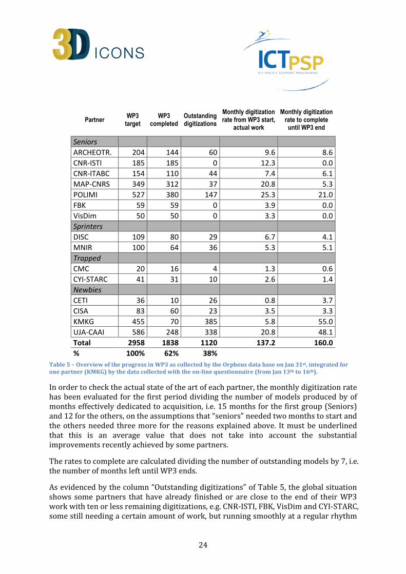
The individual and global situation is shown in Table 5, where we see a global

performance of 1,838 items acquired (62%) against 1,120 to be completed (38%) to

reach the total of 2,958 3D digitizations. The difference in work required to produce

new models or to adjust existing ones is not taken into account in the table. The status

of pre-existing models is difficult to analyze: in some cases they were ready for delivery,

in others some work was still required, for example validating 3D and sometimes re-

processing it. As it is impossible to exactly quantify the amount of work dedicated to

this task, the table is necessarily approximate.

This global value, at project level, might be interpreted as evidence of a delay in the

progress in the first 17 months of the 24 available, corresponding approximately to

71% elapsed time, which would be the amount of work done to be perfectly on schedule.

Such percentages do not however keep into account differences among partners and

their respective tasks that are difficult to quantify. Therefore, the table must be

accompanied by a qualitative explanation.

It should be considered that in the initial phase of WP3, some of the units – especially

those less technically skilled or experienced - needed time for setting up the most

optimized 3D acquisition strategy, tailored to the work each unit is expected to carry

out in the WP3 period. This will be analyzed in detail below.

23

At project level, let us consider, therefore, an average of 2 months’ initial phase, with

very low productivity due to the start-up of this unprecedented massive 3D acquisition

activity. Thus the operating months at full rate are about 15, which compared with the

duration of the Work Package gives about 62%, as actually performed by the project.

This is relevant for the next months, when the activity will proceed at the steady level

achieved by now.

As regards individual partners, there is a significant difference from each other.

For a first group of partners, the “seniors”, i.e. ARCHAEOTRANSFER, CNR (both teams),

MAP-CNRS and POLIMI, content to be provided included about one third of already

available models. This witnesses their previous experience in 3D acquisition and in

defining a mass digitization strategy. This enabled them to start quickly the preparation

of new models. Thus they have a very high production rate, as they could use almost all

the time since the start of WP3, with a very short ‘warm-up’.

FBK and VisDim also belong to the “senior” group. Their production rate is only

apparently low: this is because they had less models to produce, as shown by the fact

that they already achieved the target completely.

A second grouping, the “sprinters”, includes MNIR, which was able to escape from an

administrative impasse and proceeded at good pace since then, and DISC, which

managed to start quickly, perhaps supported by a very effective national strategy on

digitization.

There is then a group of two rather experienced partners, the “trapped” ones, CYI and

CMC, hampered by external problems. For example, as regards CYI, the use of some

already made models was forbidden because of an unforeseen change of policy of the

local antiquity authority, which all of a sudden stopped also the acquisition of other

models, and by political difficulties in the data acquisition in the UN controlled area,

which could be completed only partially. Both partners are actively searching for

substitutes, and they are expected to recover, at least partially, the time lost in useless

negotiations. For these partners the relatively low scanning rate in the first period of

activity is due to the external difficulties: they did not operate at full speed for several

months; actually in these months they could not operate at all.

Finally there are the “newbies”: CETI, CISA, KMKG, and UJA-CAAI. All these partners had

previous sporadic experience in digitization: they all have zero or few pre-existing

models, with the exception of CISA. They all needed some initial time to get acquainted

with the tools and to establish an appropriate digitization pipeline for mass acquisition.

Their contents differ: KMKG and UJA-CAAI will digitize small objects such as museum

artifacts and archaeological finds, a simpler task than CETI and CISA, which will work on

more complex monuments. For all of them, and more sensibly for KMKG and UJA-CAAI,

the rate of improvement of the last few months shows that they are now able to

perform much better, increasing substantially their digitization rate.

24

Partner WP3 target

WP3 completed

Outstanding digitizations

Monthly digitization rate from WP3 start,

actual work

Monthly digitization rate to complete until WP3 end

Seniors

ARCHEOTR. 204 144 60 9.6 8.6

CNR-ISTI 185 185 0 12.3 0.0

CNR-ITABC 154 110 44 7.4 6.1

MAP-CNRS 349 312 37 20.8 5.3

POLIMI 527 380 147 25.3 21.0

FBK 59 59 0 3.9 0.0

VisDim 50 50 0 3.3 0.0

Sprinters

DISC 109 80 29 6.7 4.1

MNIR 100 64 36 5.3 5.1

Trapped

CMC 20 16 4 1.3 0.6

CYI-STARC 41 31 10 2.6 1.4

Newbies

CETI 36 10 26 0.8 3.7

CISA 83 60 23 3.5 3.3

KMKG 455 70 385 5.8 55.0

UJA-CAAI 586 248 338 20.8 48.1

Total 2958 1838 1120 137.2 160.0

% 100% 62% 38%

Table 5 – Overview of the progress in WP3 as collected by the Orpheus data base on Jan 31st, integrated for

one partner (KMKG) by the data collected with the on-line questionnaire (from Jan 13th to 16th).

In order to check the actual state of the art of each partner, the monthly digitization rate

has been evaluated for the first period dividing the number of models produced by of

months effectively dedicated to acquisition, i.e. 15 months for the first group (Seniors)

and 12 for the others, on the assumptions that “seniors” needed two months to start and

the others needed three more for the reasons explained above. It must be underlined

that this is an average value that does not take into account the substantial

improvements recently achieved by some partners.

The rates to complete are calculated dividing the number of outstanding models by 7, i.e.

the number of months left until WP3 ends.

As evidenced by the column “Outstanding digitizations” of Table 5, the global situation

shows some partners that have already finished or are close to the end of their WP3

work with ten or less remaining digitizations, e.g. CNR-ISTI, FBK, VisDim and CYI-STARC,

some still needing a certain amount of work, but running smoothly at a regular rhythm

25

(ARCHEOTR., CNR-ITABC, MAP-CNRS, POLIMI, DISC, MNIR), whose digitization rate

does not need to increase. In fact, some of these partners will be available to support the

delayed ones if necessary.

Other partners, the “newbies”, will need to increase their efficiency, as they have

already started doing recently:

- CETI and CISA (whose monthly digitization rate would be close to that of CETI

without taking into account his preexisting models) should arrive at a rate close

to the one MNIR and DISC have already achieved to finish their work by M30. A

rate of less than 5 models/month sounds reasonable for both of them, keeping

into account that their outstanding work is a mixture of small and large

monuments.

- KMKG and UJA-CAAI should much improve their performance, this seems

feasible (although perhaps not easy) when considering that their content

consists of small objects for which the digitization is fast when an optimized

production pipeline is adopted. Experience shows that an average of 4-5 objects

per day may be maintained. In any case, limited delays may be absorbed with

little impact by the remaining 6 months after WP3 completion.

It must be underlined that the WP3 questionnaire mentioned above, regarding this

particular point contained the question “Are you confident to reach WP3 goal?” and all

partners answered “yes”, expressing their commitment for obtaining the planned

results.

Regarding the final project goal, some partners have added new models to their original

lists, others had made substitutions mainly due to problems with IPR. This will be

covered in more detail in the Year 2 Management Report where the changes will be

summarized. These adjustments generated a zero balance with respect to the target

reported in the DOW, but the analysis reported above shows that some of the partners

have the capability to possibly exceed the DOW limit, becoming a possible backup

resource in case of difficulties of the “newbies”.

In conclusion, with the exception of a very few potentially critical cases, we can state

that if the project will globally accelerate, increasing of the 20% (x1,2) the average rate

of digitization/month provided in the first 17 month of activity - that given the previous

considerations seems definitely feasible - the WP3 activity can be properly concluded as

planned within M30. Since some flexibility was built into the original schedule with a

further six months before 3D-ICONS finishes, any minor delays can be easily absorbed

enabling the delivery of metadata and 3D models to complete on time at M36.

26

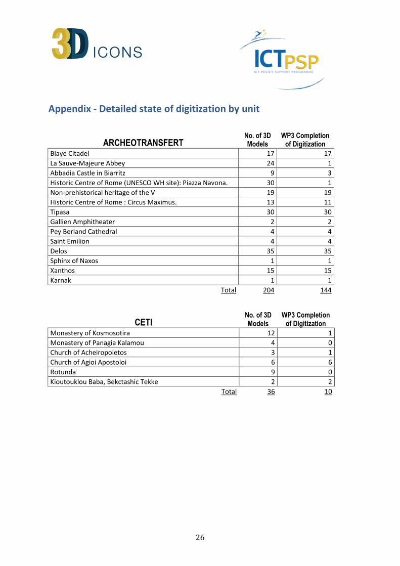
Appendix - Detailed state of digitization by unit

ARCHEOTRANSFERT No. of 3D Models

WP3 Completion of Digitization

Blaye Citadel 17 17

La Sauve-Majeure Abbey 24 1

Abbadia Castle in Biarritz 9 3

Historic Centre of Rome (UNESCO WH site): Piazza Navona. 30 1

Non-prehistorical heritage of the V 19 19

Historic Centre of Rome : Circus Maximus. 13 11

Tipasa 30 30

Gallien Amphitheater 2 2

Pey Berland Cathedral 4 4

Saint Emilion 4 4

Delos 35 35

Sphinx of Naxos 1 1

Xanthos 15 15

Karnak 1 1

Total 204 144

CETI No. of 3D Models


Monastery of Kosmosotira 12 1

Monastery of Panagia Kalamou 4 0

Church of Acheiropoietos 3 1

Church of Agioi Apostoloi 6 6

Rotunda 9 0

Kioutouklou Baba, Bekctashic Tekke 2 2

Total 36 10

27

CISA No. of 3D Models


Historical Center of Naples: Roman Theatre 2 1

Historical Center of Naples: Statue of Herakles Farnese 1 1

Historical Center of Naples: Necropolis 4 0

Historical Center of Naples: Walls 1 1

Historical Center of Naples. Thermae 4 0

Pompeii: Necropolis 4 0

Pompeii: Villa of Misteri 3 0

Pompeii: Casa del Fauno 3 0

Hercolaneum: Theater 3 0

Hercolaneum: Shrine of Augustali House 7 7

Hercolaneum: Roman Boat 1 0

Etruscan artifacts 50 50

Total 83 60

CMC No. of 3D Models


Skara Brae E1 11 11

Skara Brae E2 2 1

Skara Brae E3 3 2

Skara Brae E4 2 1

Skara Brae E5 2 1

Skara Brae Artefacts 0 0

Total 20 16

28

CNR-ISTI No. of 3D Models


Loggia dei Lanzi 8 8

Piazza della Signoria 12 12

Tempio di Luni 20 20

Piazza dei Cavalieri 4 4

San Gimignano 10 10

Certosa di Calci 2 2

Badia Camaldolese 4 4

Ara Pacis 5 5

Duomo di Pisa 26 26

Portalada 4 4

Ipogeo dei Tetina 24 24

David Donatello (marble version) 4 4

Sarcofago degli Sposi 6 6

Ruthwell Cross 14 14

Pompeii 16 16

Villa Medicea Montelupo 3 3

San Leonardo in Arcetri 14 14

Capsella Samagher 4 4

DELOS statues (new since targets set) 5 5

Total 185 185

CNR-ITABC No. of 3D Models


Historical Centre of Rome 27 15

Cerveteri necropolis 17 1

Appia Archaeological Park 29 22

Villa of Livia 52 52

Sarmizegetusa 9 0

Via Flaminia 11 11

Villa of Volusii 4 4

Lucus Feroniae 1 1

Estense Castle 4 4

Total 154 110

29

CYI-STARC No. of 3D Models


Hellenistic-Roman Paphos Theatre 21 20

Ayia Marina church in Derynia, Famagusta District (Buffer

Zone) 11 11

CYI-STARC - The Santa Cristina archaeological area,

Paulilatino 4 0

CYI-STARC - The Cenacle (room of last supper), Israel 5 0

Total 41 31

DISC No. of 3D Models


BNB_LANDSCAPE 3 3

TARA 10 10

DA_ROYAL 1 1

NAVAN_ROYAL 1 1

RATH_ROYAL 1 0

SKELLIG 13 12

POULNABRONE 1 1

BNB_KNW 16 14

DUN_AONGHASA 4 4

BNB_NG 5 0

DUN_EOCHLA 1 0

DUN_EOGHANACHTA 1 0

DUCATHAIR 1 0

STAIGUE 1 1

AN_GRIANAN 1 0

CAHERGAL 1 1

CLONMACNOISE 16 11

DERRY_WALLS 8 3

GLENDALOUGH 16 16

GALLARUS_ORATORY 1 1

DROMBEG 1 1

- 1 0

- 1 0

- 1 0

- 3 0

Total 109 80

30

FBK

No. of 3D Models


Three Peaks of Lavaredo 1 1

Buonconsiglio Castle 3 3

Buonconsiglio Castle Museum 8 8

Drena Castle 1 1

Etruscan Tombs 12 12

Valer Castle 3 3

Stenico Castle 1 1

Paestum Archeological Site 6 6

Paestum Archeological Museum 6 6

Etruscan Museum - Roma Villa Giulia 2 2

Etruscan Museum - Vulci 4 4

Etruscan Museum - Chianciano 10 10

Ventimiglia Theatre 1 1

Austro-Hungarian Forts 1 1

Total 59 59

KMKG No. of 3D Models


Almeria Necropolis 450 70

Cabezo del Ofício, grave 12 1 0


Zapata, grave 15 1 0


Cabezo del Oficio, grave 18 1 0

Total 455 70

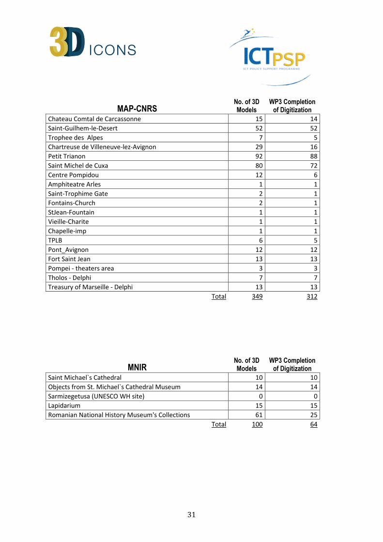
31

MAP-CNRS No. of 3D Models


Chateau Comtal de Carcassonne 15 14

Saint-Guilhem-le-Desert 52 52

Trophee des Alpes 7 5

Chartreuse de Villeneuve-lez-Avignon 29 16

Petit Trianon 92 88

Saint Michel de Cuxa 80 72

Centre Pompidou 12 6

Amphiteatre Arles 1 1

Saint-Trophime Gate 2 1

Fontains-Church 2 1

StJean-Fountain 1 1

Vieille-Charite 1 1

Chapelle-imp 1 1

TPLB 6 5

Pont_Avignon 12 12

Fort Saint Jean 13 13

Pompei - theaters area 3 3

Tholos - Delphi 7 7

Treasury of Marseille - Delphi 13 13

Total 349 312

MNIR No. of 3D Models


Saint Michael`s Cathedral 10 10

Objects from St. Michael`s Cathedral Museum 14 14

Sarmizegetusa (UNESCO WH site) 0 0

Lapidarium 15 15

Romanian National History Museum's Collections 61 25

Total 100 64

32

POLIMI No. of 3D Models


Chartreuse of Pavia (6 separate monuments) 46 46

The roman church of San Giovanni in Conca (Milan) 9 9

Civico Museo Archeologico di Milano 472 325

Total 527 380

UJA-CAAI No. of 3D Models


Oppidum Puente Tablas 28 28

Cemetery of La Noria (Fuente de Piedra, Málaga) 52 52

Cemetery of Piquias (Arjona, Jaén) 47 47

Sculptoric group of Porcuna 81 40

Burial Chamber of Toya (Jaén) 3 0

Rockshelter of Engarbo I and II (Santiago-Pontones, Jaén) 4 2

Cemetery and site of Tutugi (Galera, Granada) 29 7

Burial Chamber of Hornos de Peal (Peal de Becerro, Jaén) 5 5

Sculptoric group of El Pajarillo 9 0

Sanctuary of Castellar 64 27

The Provincial Museum of Jaén 150 16

The archaeological site and the museum of Castulo 60 0

Hill of Albahacas 52 22

Wall of Ibros 1 1

Wall of Cerro Miguelico 1 1

Total 586 248

VisDim No. of 3D Models


Historical reconstruction of Ename village, Belgium 50 50

Total 50 50

3D-ICONS- D3 1: Interim Report on Data Acquisition

Internet

Transcript of 3D-ICONS- D3 1: Interim Report on Data Acquisition