3D Geometry for Computer Graphics. 2 The plan today Least squares approach General / Polynomial...
38
3D Geometry for Computer Graphics
-
date post
19-Dec-2015 -
Category
Documents
-
view
220 -
download
2
Transcript of 3D Geometry for Computer Graphics. 2 The plan today Least squares approach General / Polynomial...

3D Geometry forComputer Graphics

2
The plan today
Least squares approach General / Polynomial fitting Linear systems of equations Local polynomial surface fitting
3
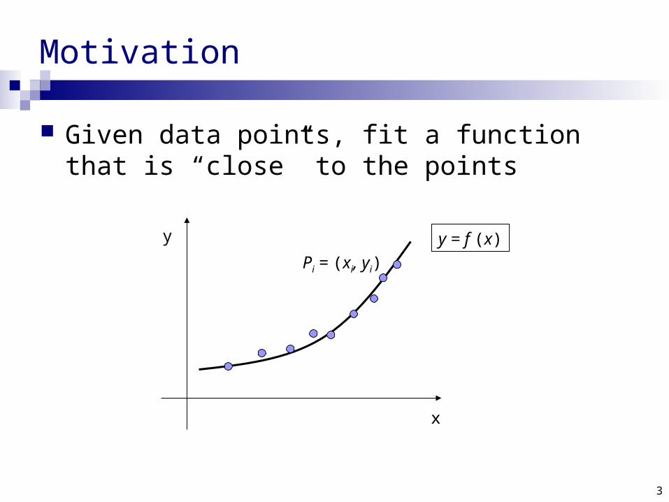
y = f (x)
Motivation
Given data points, fit a function that is “close” to the points
y
x
Pi = (xi, yi)

4
Motivation
Local surface fitting to 3D points

5
Line fitting
Orthogonal offsets minimization – we already learned (PCA)
x
y

6
Line fitting
y-offsets minimization
x
y
Pi = (xi, yi)

7
Line fitting
Find a line y = ax + b that minimizes
E(a,b) is quadratic in the unknown parameters a, b
Another option would be, for example:
But – it is not differentiable, harder to minimize…
2
1
( , ) [ ( )]n
i ii
a b ay bE x
n
iii baxybaAbsErr
1
)(),(
8
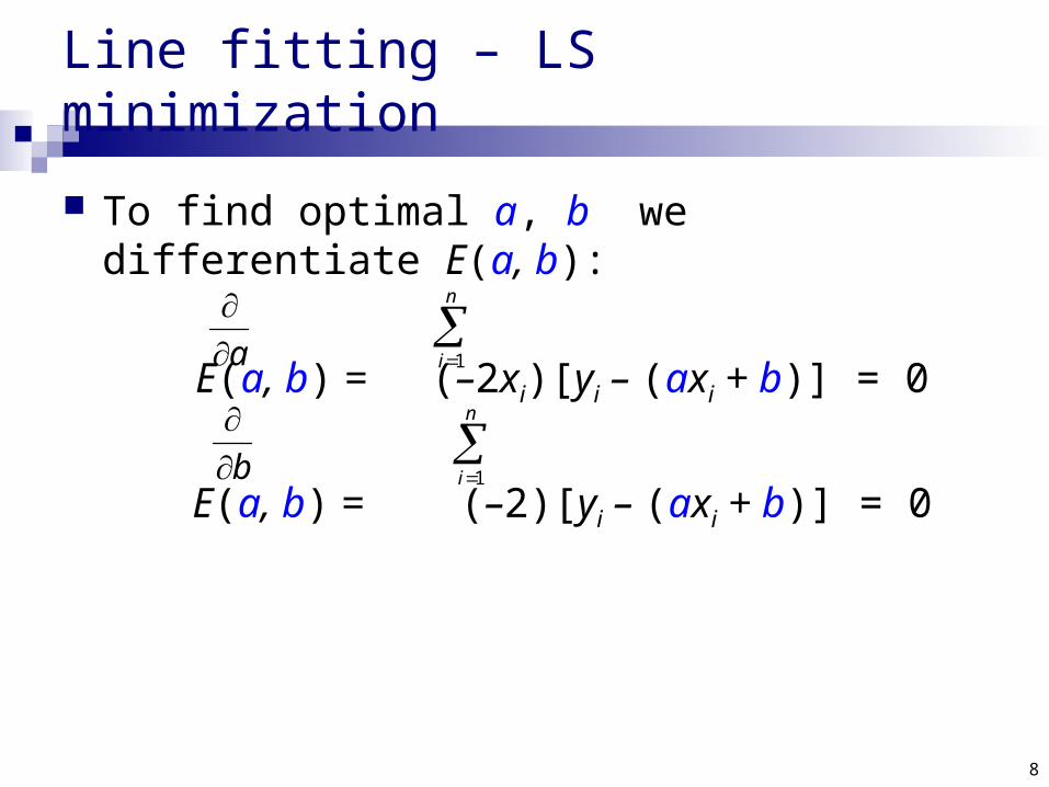
Line fitting – LS minimization
To find optimal a, b we differentiate E(a, b):
E(a, b) = (–2xi)[yi – (axi + b)] = 0
E(a, b) = (–2)[yi – (axi + b)] = 0
a
n
i 1
n
i 1b

9
Line fitting – LS minimization
We get two linear equations for a, b:
(–2xi)[yi – (axi + b)] = 0
(–2)[yi – (axi + b)] = 0
n
i 1
n
i 1

10
Line fitting – LS minimization
We get two linear equations for a, b:
[xiyi – axi2 – bxi] = 0
[yi – axi – b] = 0
n
i 1
)1(
n
i 1
)2(

11
Line fitting – LS minimization
We get two linear equations for a, b:
( xi2) a + ( xi) b = xiyi
( xi) a + ( 1) b = yi
n
i 1
n
i 1
n
i 1
n
i 1
n
i 1
n
i 1

12
Line fitting – LS minimization
Solve for a, b using e.g. Gauss elimination
Question: why the solution is the minimum for the error function?
E(a, b) = [yi – (axi + b)]2
n
i 1

13
Fitting polynomials
y
x

14
Decide on the degree of the polynomial, k Want to fit f (x) = akx
k + ak-1xk-1 + … + a1x+ a0
Minimize:
E(a0, a1, …, ak) = [yi – (akxik+ak-1xi
k-1+ …+a1xi+a0)]2
E(a0,…,ak) = (– 2xm)[yi – (akxik+ak-1xi
k-1+…+ a0)] = 0
Fitting polynomials
n
i 1
n
i 1ma

15
Fitting polynomials
We get a linear system of k+1 in k+1 variables
1 1 1 1
2 1
1 1 1 1
1 2
1 1
0
1 1
1
1 1n n n n
ki i i
i i i i
n n n nk
i i i i ii i i i
n n n nk k k k
i i i i ii i i
ki
x x y
x x x x
a
a
a
y
x x x x y
16
General parametric fitting
We can use this approach to fit any function f(x) Specified by parameters a, b, c, … The expression f(x) linearly depends on the
parameters a, b, c, …

17
General parametric fitting
Want to fit function fabc…(x) to data points (xi, yi)
Define E(a,b,c,…) = [yi – fabc…(xi)]2
Solve the linear system
...1
...1
( , , , ) ( 2 ( ))[ ( )] 0
( , , , ) ( 2 ( ))[ ( )] 0
n
abc i i ii
n
abc i i ii
E a b c f x y f xa a
E a b c f x y f xb b
n
i 1

18
General parametric fitting
It can even be some crazy function like
Or in general:
2
222
71 3
1( ) sinx
f x x x e
1 2, , 1..., 1 2 2( ) ( ) ( ) ... ( )k kkf x f x f x f x

19
Solving linear systems in LS sense
Let’s look at the problem a little differently: We have data points (xi, yi)
We want the function f(x) to go through the points:
i =1, …, n: yi = f(xi)
Strict interpolation is in general not possible In polynomials: n+1 points define a unique interpolation
polynomial of degree n. So, if we have 1000 points and want a cubic polynomial, we
probably won’t find it…

20
Solving linear systems in LS sense
We have an over-determined linear system nk:
f(x1) = 1 f1(x1) + 2 f2(x1) + … + k fk(x1) = y1
f(x2) = 1 f1(x2) + 2 f2(x2) + … + k fk(x2) = y2
…
…
…
f(xn) = 1 f1(xn) + 2 f2(xn) + … + k fk(xn) = yn

21
Solving linear systems in LS sense
In matrix form:
1 1 2 1 1 1
1 2 2 2 2 2
1 2
( ) ( ) ... ( )
( ) ( ) ... ( )
...
( ) ( ) ... ( )
k
k
n n k n n
f x f x f x y
f x f x f x y
f x f x f x y
1
2
k
22
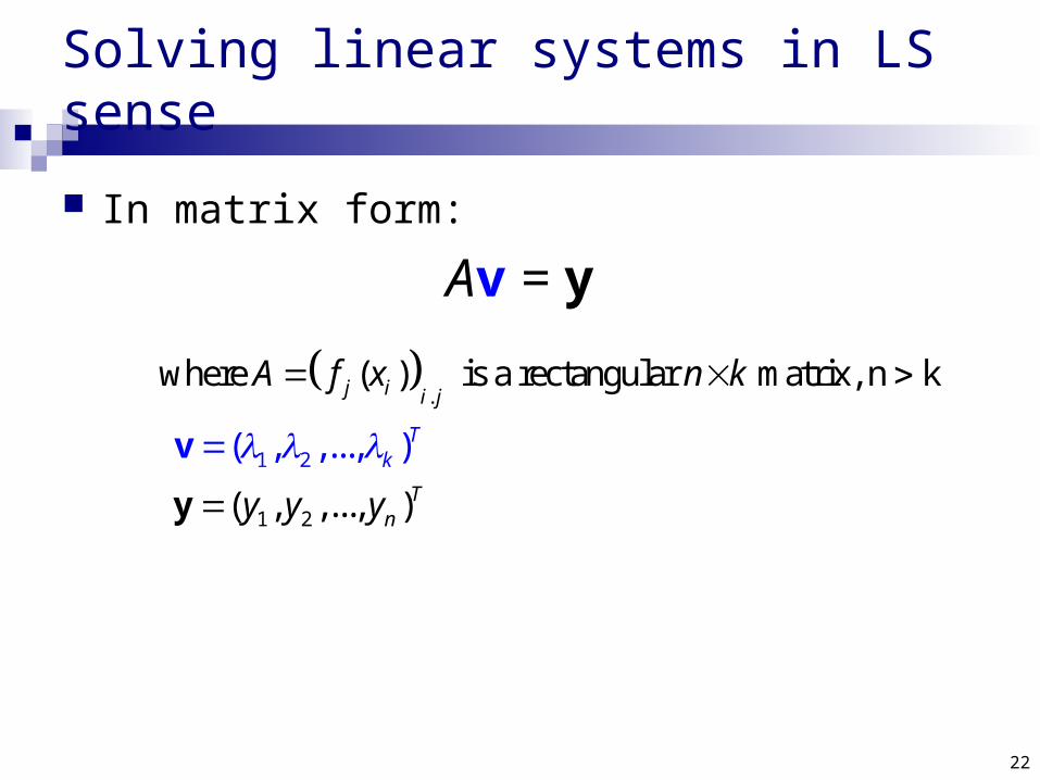
Solving linear systems in LS sense
In matrix form:
Av = y
.
1 2
1 2
where ( ) is a rectangular matr
( , ,...,
ix, n k
( , ,..., )
)
j j
T
i i
n
k
T
A f x n k
y y y
y
v

23
Solving linear systems in LS sense
More constrains than variables – no exact solutions generally exist
We want to find something that is an “approximate solution”:
2arg min A
vv v y

24
Finding the LS solution
v Rk
Av Rn As we vary v, Av varies over the linear
subspace of Rn spanned by the columns of A:
Av = A2A1 Ak
1
2
.
. k
= 1A 1 A 2 A k + 2 +…+ k
25
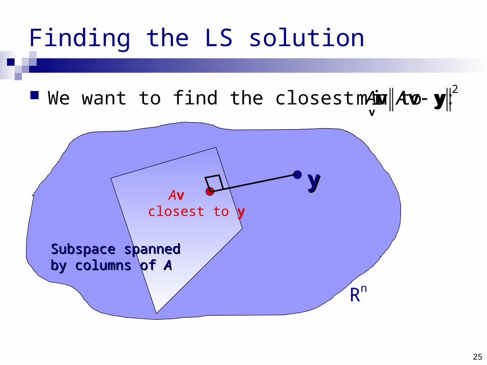
Finding the LS solution
We want to find the closest Av to y:2
min A v
v y
Subspace spannedSubspace spannedby columns of by columns of AA
yy
Rn
Avclosest to y

26
Finding the LS solution
The vector Av closest to y satisfies:
(Av – y) {subspace of A’s columns}
column Ai, <Ai, Av – y> = 0
i, AiT(Av – y) = 0
AT(Av – y) = 0
(ATA)v = ATy
These arecalled the
normal equations

27
Finding the LS solution
We got a square symmetric system (ATA)v = ATy (kk)
If A has full rank (the columns of A are linearly independent) then (ATA) is invertible.
2
1
min
( )T T
A
A A A
vv y
v y
28
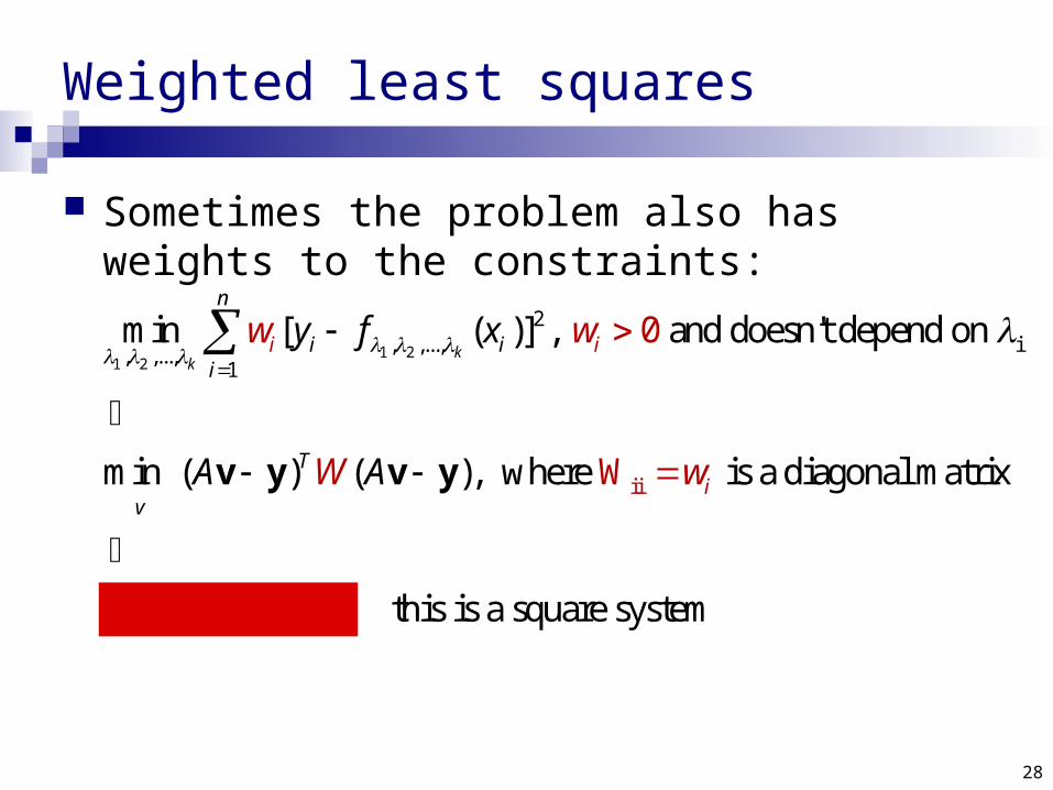
Weighted least squares
Sometimes the problem also has weights to the constraints:
1 21 2
2, ,..., i, ,. ,
ii
..1
min [ ( )] , and doesn't depend on
min ( ) ( ), where is a diagonal matrix
( ) this is a
0
s
W
quare system
kk
n
i i i
Ti
T
ii
v
T
w w
W
y f x
A A
A A v A y
w
W W
v y v y

29
Local surface fitting to 3D points
Normals? Lighting? Upsampling?

30
Local surface fitting to 3D points
Locally approximate
a polynomial surface
from points

31
Fitting local polynomial
X Y
ZReference plane
Fit a local polynomial around a point P
P

32
Fitting local polynomial surface
Compute a reference plane that fits the points close to P Use the local basis defined by the normal to the plane!
z
x y

33
Fitting local polynomial surface
Fit polynomial z = p(x,y) = ax2 + bxy + cy2 + dx + ey + f
z
x y

34
Fitting local polynomial surface
Fit polynomial z = p(x,y) = ax2 + bxy + cy2 + dx + ey + f
z
x
y

35
Fitting local polynomial surface
Fit polynomial z = p(x,y) = ax2 + bxy + cy2 + dx + ey + f
z
x y

36
Fitting local polynomial surface
Again, solve the system in LS sense:
ax12 + bx1y1 + cy1
2 + dx1 + ey1 + f = z1
ax22 + bx2y2 + cy2
2 + dx2 + ey2 + f = z1
. . .
axn2 + bxnyn + cyn
2 + dxn + eyn + f = zn
Minimize ||zi – p(xi, yi)||2
37
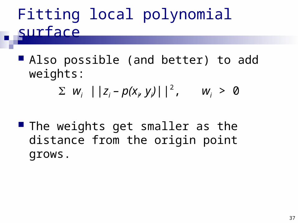
Fitting local polynomial surface
Also possible (and better) to add weights:
wi ||zi – p(xi, yi)||2, wi > 0
The weights get smaller as the distance from the origin point grows.

See you next time