
3D elastic wave propagation modelling in the presence … · 3D elastic wave propagation modelling...
18
3D elastic wave propagation modelling in the presence of 2D fluid-filled thin inclusions Anto ´nio Tadeu * , Paulo Amado Mendes, Julieta Anto ´nio Department of Civil Engineering, University of Coimbra, Po ´lo II, Pinhal de Marrocos, 3030-290 Coimbra, Portugal Received 17 January 2005; received in revised form 6 June 2005; accepted 22 August 2005 Abstract In this paper, the traction boundary element method (TBEM) and the boundary element method (BEM), formulated in the frequency domain, are combined so as to evaluate the 3D scattered wave field generated by 2D fluid-filled thin inclusions. This model overcomes the thin-body difficulty posed when the classical BEM is applied. The inclusion may exhibit arbitrary geometry and orientation, and may have null thickness. The singular and hypersingular integrals that appear during the model’s implementation are computed analytically, which overcomes one of the drawbacks of this formulation. Different source types such as plane, cylindrical and spherical sources, may excite the medium. The results provided by the proposed model are verified against responses provided by analytical models derived for a cylindrical circular fluid-filled borehole. The performance of the proposed model is illustrated by solving the cases of a flat fluid-filled fracture with small thickness and a fluid-filled S- shaped inclusion, modelled with both small and null thickness, all of which are buried in an unbounded elastic medium. Time and frequency responses are presented when spherical pulses with a Ricker wavelet time evolution strikes the cracked medium. To avoid the aliasing phenomena in the time domain, complex frequencies are used. The effect of these complex frequencies is removed by rescaling the time responses obtained by first applying an inverse Fourier transformation to the frequency domain computations. The numerical results are analysed and a selection of snapshots from different computer animations is given. This makes it possible to understand the time evolution of the wave propagation around and through the fluid-filled inclusion. q 2005 Elsevier Ltd. All rights reserved. Keywords: Wave propagation; Elastic scattering; Fluid-filled thin inclusions; Boundary element method; Traction boundary element method; 2.5D problem 1. Introduction It is essential to fully understand how waves propagate from the source to the receiver if the signals recorded during seismic testing can themselves be understood. The relative contribution of the many wave propagation modes that may be excited by the source determines the complexity of the wave patterns recorded at the receivers. This contribution depends on the distance from the source to the receiver, the dominant frequency of the pulse, the material characteristics of the geologic formation, the type of source and the presence of fractures (cracks) [1–3]. Cracks are very important in several fields, such as determining the integrity of construction elements (in many engineering applications), and detecting and defining delamination in slabs and pavements using non- destructive evaluation techniques [4–8]. Various numerical methods have been used to study wave scattering by inclusions and thin heterogeneities, since analytical solutions are only known for simple problems [9,10]. The finite difference method (FDM) [11–16], the finite element method (FEM) [17–19], the boundary integral approach [20], the boundary element method (BEM) [21,22] and hybrid methods [23–25] are some of the techniques most often used. In an unbounded medium the BEM is particularly efficient since it automatically satisfies the far field conditions, it can easily handle irregular geometries and only requires the discretization of the material interfaces, which is an advantage over other numerical techniques such as the FDM and the FEM. However, the BEM degenerates when thin or even null- thickness inclusions occur. Pointer et al. [7] proposed an indirect boundary element formulation to simulate the seismic wave field scattered from an arbitrary number of fractures that are either empty or contain Engineering Analysis with Boundary Elements 30 (2006) 176–193 www.elsevier.com/locate/enganabound 0955-7997/$ - see front matter q 2005 Elsevier Ltd. All rights reserved. doi:10.1016/j.enganabound.2005.08.014 * Corresponding author. Tel.: C351 239 797201; fax: C351 239 797190. E-mail address: [email protected] (A. Tadeu).
Transcript of 3D elastic wave propagation modelling in the presence … · 3D elastic wave propagation modelling...
3D elastic wave propagation modelling in the presence of 2D
fluid-filled thin inclusions
Antonio Tadeu *, Paulo Amado Mendes, Julieta Antonio
Department of Civil Engineering, University of Coimbra, Polo II, Pinhal de Marrocos, 3030-290 Coimbra, Portugal
Received 17 January 2005; received in revised form 6 June 2005; accepted 22 August 2005
Abstract
In this paper, the traction boundary element method (TBEM) and the boundary element method (BEM), formulated in the frequency domain,
are combined so as to evaluate the 3D scattered wave field generated by 2D fluid-filled thin inclusions. This model overcomes the thin-body
difficulty posed when the classical BEM is applied. The inclusion may exhibit arbitrary geometry and orientation, and may have null thickness.
The singular and hypersingular integrals that appear during the model’s implementation are computed analytically, which overcomes one of the
drawbacks of this formulation. Different source types such as plane, cylindrical and spherical sources, may excite the medium. The results
provided by the proposed model are verified against responses provided by analytical models derived for a cylindrical circular fluid-filled
borehole.
The performance of the proposed model is illustrated by solving the cases of a flat fluid-filled fracture with small thickness and a fluid-filled S-
shaped inclusion, modelled with both small and null thickness, all of which are buried in an unbounded elastic medium. Time and frequency
responses are presented when spherical pulses with a Ricker wavelet time evolution strikes the cracked medium. To avoid the aliasing phenomena
in the time domain, complex frequencies are used. The effect of these complex frequencies is removed by rescaling the time responses obtained by
first applying an inverse Fourier transformation to the frequency domain computations. The numerical results are analysed and a selection of
snapshots from different computer animations is given. This makes it possible to understand the time evolution of the wave propagation around
and through the fluid-filled inclusion.
q 2005 Elsevier Ltd. All rights reserved.
Keywords: Wave propagation; Elastic scattering; Fluid-filled thin inclusions; Boundary element method; Traction boundary element method; 2.5D problem
1. Introduction
It is essential to fully understand how waves propagate from
the source to the receiver if the signals recorded during seismic
testing can themselves be understood. The relative contribution
of the many wave propagation modes that may be excited by
the source determines the complexity of the wave patterns
recorded at the receivers. This contribution depends on the
distance from the source to the receiver, the dominant
frequency of the pulse, the material characteristics of the
geologic formation, the type of source and the presence of
fractures (cracks) [1–3]. Cracks are very important in several
fields, such as determining the integrity of construction
elements (in many engineering applications), and detecting
0955-7997/$ - see front matter q 2005 Elsevier Ltd. All rights reserved.
doi:10.1016/j.enganabound.2005.08.014
* Corresponding author. Tel.: C351 239 797201; fax: C351 239 797190.
E-mail address: [email protected] (A. Tadeu).
and defining delamination in slabs and pavements using non-
destructive evaluation techniques [4–8].
Various numerical methods have been used to study wave
scattering by inclusions and thin heterogeneities, since
analytical solutions are only known for simple problems
[9,10]. The finite difference method (FDM) [11–16], the finite
element method (FEM) [17–19], the boundary integral
approach [20], the boundary element method (BEM) [21,22]
and hybrid methods [23–25] are some of the techniques most
often used.
In an unbounded medium the BEM is particularly efficient
since it automatically satisfies the far field conditions, it can
easily handle irregular geometries and only requires the
discretization of the material interfaces, which is an advantage
over other numerical techniques such as the FDM and the
FEM. However, the BEM degenerates when thin or even null-
thickness inclusions occur.
Pointer et al. [7] proposed an indirect boundary element
formulation to simulate the seismic wave field scattered from
an arbitrary number of fractures that are either empty or contain
Engineering Analysis with Boundary Elements 30 (2006) 176–193
www.elsevier.com/locate/enganabound
A. Tadeu et al. / Engineering Analysis with Boundary Elements 30 (2006) 176–193 177
elastic or fluid material. The traction boundary integral
equation method is a different technique that handles the
thin-body difficulty [26–29]. The appearance of hypersingular
integrals is one of the difficulties posed by these formulations.
Different attempts have been made to overcome this difficulty
[30–33]. The traction boundary element method (TBEM) was
used by Prosper [34] and Prosper and Kausel [35] to model the
scattering of waves by flat and horizontal empty cracks of zero
thickness in elastic media. An indirect approach was proposed
for the analytical evaluation of integrals with hypersingular
kernels for plane-strain cases in the 2D problem.
Most of the work published refers to the cases of 2D and, in
some cases, 3D geometries and where the crack is assumed to
be empty (free stress field). In real life, the crack may be either
empty or it may be filled with fluid or elastic material, which
determines a distinct dynamic behaviour.
This work solves the case of a crack whose geometry does
not change along one direction (2D) while the source exhibits
a 3D nature. This geometry is commonly referred to as a two-
and-a-half-dimensional problem (2-1/2D). The solution is
obtained after applying a spatial Fourier transform along the
direction in which the geometry remains constant. This
procedure allows the 3D solution to be computed as a
summation of 2D solutions for different spatial wavenumbers.
Furthermore, the crack is assumed to be filled with fluid,
which determines the continuity of normal displacements and
normal tractions, and null tangential stresses along the
boundary of the crack. The crack may have a small or even
null thickness.
The problem is solved using a mixed formulation involving
the application of both the TBEM and the BEM: one of the
formulations is used for the upper surface of the crack while
the other models its lower surface. As noted above, the use
of the TBEM leads to the integration of hypersingular kernels.
In the work described in this paper, these hypersingular kernels
are evaluated analytically using an indirect approach, which is
accomplished by defining the dynamic equilibrium of semi-
cylinders above the boundary elements, discretizing the crack.
It represents an extension of the work by Prosper and Kausel
[35], when they defined the behaviour of a 2D dimensional flat
and horizontal crack. The combination of the displacement
BEM and the traction BEM is commonly referred to as the
‘Dual Boundary Element Method’ [36–38].
In this paper, the 3D problem is defined and its solution
described, and the boundary element formulations (BEM,
TBEM and TBEMCBEM) are presented. Then the numerical
solutions are verified against analytical solutions known for the
case of a cylindrical circular fluid-filled borehole. The
procedure for finding time signatures is outlined. The paper
ends with an illustration of the applicability of the proposed
technique to simulate the 3D wave propagation in the vicinity
of fluid-filled thin inclusions.
2. Problem formulation
An unbounded homogeneous isotropic elastic medium, with
no intrinsic attenuation, hosts a 2D fluid–filled inclusion.
The hosting medium has density r and allows shear wave and
compressional wave velocities of b and a, respectively.
A Cartesian coordinate system is used with the z-axis being
aligned along the direction in which the geometry of the
inclusion remains constant. The inclusion is assumed to be
filled with an inviscid fluid with density rf, where the
compressional waves propagate with a velocity of af. A
dilatational point source, placed in the host medium at position
(xs, ys, zs) and oscillating with frequency u, emits an incident
field that can be expressed by the dilatational potential f,
finc ZAeiðu=aÞðatK
ffiffiffiffiffiffiffiffiffiffiffiffiffiffiffiffiffiffiffiffiffiffiffiffiffiffiffiffiffiffiffiffiffiffiffiðxKxsÞ
2CðyKysÞ2CðzKzsÞ
2p
ÞffiffiffiffiffiffiffiffiffiffiffiffiffiffiffiffiffiffiffiffiffiffiffiffiffiffiffiffiffiffiffiffiffiffiffiffiffiffiffiffiffiffiffiffiffiffiffiffiffiffiffiffiffiffiffiffiffiffiffiffiðxKxsÞ
2 C ðyKysÞ2 C ðzKzsÞ
2p ; (1)
where the subscript inc represents the direct incident field, A
the wave amplitude and iZffiffiffiffiffiffiK1
p.
In the problems where the geometry remains constant along
one direction, the 3D solution may be computed after applying a
Fourier transformation along that direction. Thus the 3D
solution is expressed as an integration of 2D problems. This
integration becomes discrete if a set of virtual sources is placed
at equal distances apart along the z direction [39]. Each of these
2D problems is solved for a specific wavenumber
kaZffiffiffiffiffiffiffiffiffiffiffiffiffiffiffiffiffiffiffiffiffiffiffiffiffiffiffiðu2=a2ÞKk2
zm
p, with Im(ka)!0, where kzmZ(2p/Lvs)m,
(mZ0,1,.,M), is the axial (in the z direction) wavenumber, and
Lvs is the distance between virtual point sources equally spaced
along z. The incident field is expressed at (x, y) by
fincðu; x; y; kzÞ ZKiA
2H0ðka
ffiffiffiffiffiffiffiffiffiffiffiffiffiffiffiffiffiffiffiffiffiffiffiffiffiffiffiffiffiffiffiffiffiffiffiffiffiffiffiðxKxsÞ
2 C ðyKysÞ2
qÞ; (2)
in which Hn(.) are second Hankel functions of order n. The
distance Lvs must be sufficiently large to prevent the virtual
sources from contributing to the response. It should be noted that
kzZ0 corresponds to the pure 2D case.
3. Different boundary integral formulations
3.1. Boundary element formulation (BEM formulation)
Considering a homogeneous elastic medium of infinite
extent, containing a fluid-filled inclusion bounded by a surface
S, and subjected to spatially sinusoidal harmonic line loads
placed in the host solid medium at xs, with spatial wavenumber
kz, the boundary integral equations can be constructed by
applying the reciprocity theorem, leading to:
– along the boundary, in the exterior domain (elastic medium)
cijuiðx0;uÞ Z
ðS
t1ðx; nn;uÞGi1ðx; x0;uÞds
K
ðS
ujðx;uÞHijðx; nn; x0;uÞds
Cuinci ðxs; x0;uÞ; (3)
A. Tadeu et al. / Engineering Analysis with Boundary Elements 30 (2006) 176–193178
– along the boundary, in the interior domain (fluid medium)
cfpðx0;uÞZ
ðS
qðx;nn;uÞGfðx;x0;uÞds
K
ðS
pðx;uÞHfðx;nn;x0;uÞds: (4)
In Eq. (3), i, jZ1, 2 stand for the normal and tangential
directions relative to the inclusion surface, respectively, while
i, jZ3 refer to the z direction. Hij(x, nn, x0, u) are the tractions
in direction j at x (on the boundary S) due to a unit point force
in direction i at x0 (the collocation point), while Gi1(x, x0, u)
are the displacements (Green’s functions) in the normal
direction at x (on the boundary S) due to a unit point force in
the direction i at x0 (the collocation point). uj(x, u) are the
displacements in direction j at x, while t1(x, nn, u) are
the tractions in the normal direction at x. uinci ðxs;x0;uÞ is the
displacement incident field at x0 along direction i. The
coefficient cij is equal to dij/2, where dij is the Kronecker
delta when the boundary is smooth. The vector nnZ(cos qn,
sin qn) is the unit outward normal at the boundary at x. In
Eq. (4), Gf(x, x0, u) and Hf(x, nn, x0, u) are, respectively,
the fundamental solutions (Green’s functions) for the pressure
p(x, u) and pressure gradient q(x, nn, u) at x due to a virtual
point pressure load at x0. The factor cf is a constant defined by
the shape of the boundary, taking the value 1/2 if x02S and S is
smooth.
The compatibility between pressure gradients and displace-
ments is obtained using the relation u1ZKð1=ru2Þðvp=vnnÞ,
while the normal pressure corresponds to normal tractions. The
boundary conditions applied along the solid–fluid interface
prescribe continuity of normal displacements and normal
tractions and null tangential stresses.
The required Green’s functions for loads and displacements
in the x, y and z directions, in the solid medium, are given in
Tadeu and Kausel [40]. The derivatives of these Green’s
functions give the following tractions along the x, y and z
directions, in the solid medium,
Hrx Z 2ma2
2b2
vGrx
vxC
a2
2b2K1
� �vGry
vyC
vGrz
vz
� �� �cos qn
CmvGry
vxC
vGrx
vy
� �sin qn
Hry Z2ma2
2b2K1
� �vGrx
vxC
vGrz
vz
� �C
a2
2b2
vGry
vy
� �sin qn
CmvGry
vxC
vGrx
vy
� �cos qn ð5Þ
Hrz Z mvGrx
vzC
vGrz
vx
� �cos qn Cm
vGry
vzC
vGrz
vy
� �sin qn;
with HrtZHrt(x, nn, x0, u), GrtZGrt(x, x0, u) and r, tZx, y, z.
These expressions can be combined to obtain Hij(x, nn, x0, u) in
the normal and tangential directions. In these equations mZrb2.
The required 2-1/2D Green’s functions for pressure and
pressure gradients in Cartesian co-ordinates are those for an
unbounded fluid medium,
Gfðx; x0;uÞ Zi
4H0ðkafrÞ
Hfðx; nn; x0;uÞ ZKi
4kafH1ðkafrÞ
vr
vnn
; (6)
in which kaf Zffiffiffiffiffiffiffiffiffiffiffiffiffiffiffiffiffiffiffiffiffiffiffiffiðu2=a2
f ÞKk2z
p, with Imðkaf
Þ!0, and
rZffiffiffiffiffiffiffiffiffiffiffiffiffiffiffiffiffiffiffiffiffiffiffiffiffiffiffiffiffiffiffiffiffiffiffiffiffiffiffiðxKx0Þ
2C ðyKy0Þ2
p.
The evaluation of these integral equations for an arbitrary
cross-section requires the discretization of both the boundary
and boundary values. By successively applying the virtual load
to each node on the boundary, a system of linear equations
relating nodal tractions (and pressures) and normal displace-
ments (and pressure gradients) is obtained, and these can be
solved for the normal tractions and nodal displacements.
The required integrations are performed in closed form
when the element to be integrated is the loaded element
[41,42], while numerical integration, using a Gaussian
quadrature scheme, applies when the element to be integrated
is not the loaded one.
3.2. Traction boundary element formulation (TBEM
formulation)
The BEM formulation described above degenerates in the
presence of a thin fluid-filled inclusion. To overcome this
difficulty the traction boundary element method (TBEM) can
be formulated [34,35], leading to the following equations:
– along the boundary, in the exterior domain (elastic medium)
ci1t1ðx0; nn;uÞCai1uiðx0;uÞ
Z
ðS
t1ðx; nn;uÞ �Gi1ðx; nn; x0;uÞds
K
ðS
ujðx;uÞ �Hijðx; nn; x0;uÞds C �uinci ðxs; x0; nn;uÞ; (7)
– along the boundary, in the interior domain (fluid medium)
afpðx0;uÞCcfqðx0; nn;uÞ
Z
ðS
qðx; nn;uÞ �Gfðx; nn; x0;uÞds
K
ðS
pðx;uÞ �Hfðx; nn; x0;uÞds: (8)
In Eq. (7), i, jZ1, 2 stand for the normal and tangential
directions relative to the inclusion surface, respectively, and i,
jZ3 refer to the z direction. These equations can be seen as
resulting from the application of dipoles (dynamic doublets).
As noted by Guiggiani [43] the coefficients ai1 and af are zero
A. Tadeu et al. / Engineering Analysis with Boundary Elements 30 (2006) 176–193 179
for piecewise straight boundary elements and ci1 is equal to 1/2,
when the boundary is smooth and iZ1, and cf is a constant
defined as above. �Gi1ðx; nn; x0;uÞ and �Hijðx; nn; x0;uÞ
are defined after the application of the traction operator to
Gi1(x, x0, u) and Hij(x, nn, x0, u). This can be seen as the
combination of the derivatives of Eq. (3), in order to x, y and z,
so as to obtain stresses �Gi1ðx; nn; x0;uÞ and �Hijðx; nn; x0;uÞ.
Along the boundary element, at x, where the unit outward
normal is defined by nnZ(cos qn, sin qn), and after the
equilibrium of stresses, the following equations are expressed
for x, y and z generated by loads also applied along x, y and z
directions:
�Gxr Z 2ma2
2b2
vGxr
vxC
a2
2b2K1
� �vGyr
vyC
vGzr
vz
� �� �cos q0
CmvGyr
vxC
vGxr
vy
� �sin q0
�Gyr Z 2ma2
2b2K1
� �vGxr
vxC
vGzr
vz
� �C
a2
2b2
vGyr
vy
� �sin q0
CmvGyr
vxC
vGxr
vy
� �cos q0
�Gzr Z mvGxr
vzC
vGzr
vx
� �cos q0 Cm
vGyr
vzC
vGzr
vy
� �sin q0 (9)
and
�Hxr Z 2ma2
2b2
vHxr
vxC
a2
2b2K1
� �vHyr
vyC
vHzr
vz
� �� �cos q0
CmvHyr
vxC
vHxr
vy
� �sin q0
�Hyr Z 2ma2
2b2K1
� �vHxr
vxC
vHzr
vz
� �C
a2
2b2
vHyr
vy
� �sin q0
CmvHyr
vxC
vHxr
vy
� �cos q0
�Hzr Z mvHxr
vzC
vHzr
vx
� �cos q0 Cm
vHyr
vzC
vHzr
vy
� �sin q0;
(10)
with n0Z(cos q0, sin q0) defining the unit outward normal at x0
(the collocation point), �Gtr Z �Gtrðx; nn; x0;uÞ, GtrZGtr(x,
x0,u), �Htr Z �Htrðx; nn; x0;uÞ, HtrZHtr(x, nn, x0,u) and r, tZx, y, z.
As for �Gtr and �Htr, the incident field component (stresses) is
obtained by analogous expressions:
�uincx Z 2m
a2
2b2
vuincx
vxC
a2
2b2K1
� �vuinc
y
vyC
vuincz
vz
� �� �cos q0
Cmvuinc
y
vxC
vuincx
vy
� �sin q0
�uincy Z2m
a2
2b2K1
� �vuinc
x
vxC
vuincz
vz
� �C
a2
2b2
vuincy
vy
� �sin q0
Cmvuinc
y
vxC
vuincx
vy
� �cos q0 ð11Þ
�uincz Z m
vuincx
vzC
vuincz
vx
� �cos q0 Cm
vuincy
vzC
vuincz
vy
� �sin q0;
with �uincr Z �uinc
r ðxs; x0; nn;uÞ; uincr Zuinc
r ðxs; x0;uÞ, and rZx, y, z.
The previous expressions can be combined so as to obtain�Gi1ðx; nn; x0;uÞ; �Hijðx; nn; x0;uÞ and �uinc
i ðxs; x0; nn;uÞ, in the
normal and tangential directions.
The required 2-1/2D Green’s functions in the fluid medium
are now defined as:
�Gfðx; nn; x0;uÞ Zi
4kafH1ðkafrÞ
vr
vx
vx
vn0
Cvr
vy
vy
vn0
� �
�Hfðx; nn; x0;uÞ
Zi
4kaf KkafH2ðkafrÞ
vr
vx
� �2 vx
vnn
Cvr
vx
vr
vy
vy
vnn
� �
CH1ðkafrÞ
r
vx
vnn
� �vx
vn0
Ci
4kaf KkafH2ðkafrÞ
vr
vx
vr
vy
vx
vnn
�C
vr
vy
� �2 vy
vnn
�
CH1ðkafrÞ
r
vy
vnn
� �vy
vn0
: (12)
The solutions of these Eqs. (7) and (8) are defined, as before, by
discretizing the boundary into N straight constant boundary
elements with the collocation points located at the center of the
elements. This leads to a set of integrations, which are
performed using a Gaussian quadrature scheme when the
element to be integrated is not the loaded element. When the
element to be integrated is the loaded one, hypersingular
integrals are defined, which are evaluated through an indirect
approach described below.
Since the final system of equations is established assuming
the normal, tangential and z directions in relation to the
boundary element, the integrations along the loaded element
are independent of its orientation. The integrations can
therefore be performed for a horizontal boundary element,
for which cos qnZcos q0Z0 and sin qnZsin q0Z1.0. These
integrations are obtained using an indirect approach, which
consists of defining the dynamic equilibrium of an isolated
semi-cylinder defined above the boundary of each boundary
element. Their derivation can be found in the Appendix A.
3.3. Dual BEM (TBEMCBEM) formulation
The two formulations can be combined so as to solve the
above problems, and the case of a thin fluid-filled inclusion.
Part of the boundary surface is loaded with monopole loads
O
R1
X
Y
R2
ff
O
R1
X
Y
O
αβρ
R1
X
Y
0.05 mR2
αf
ρf
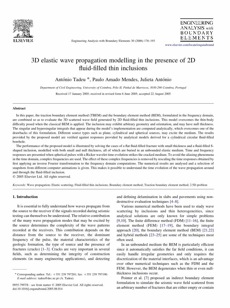
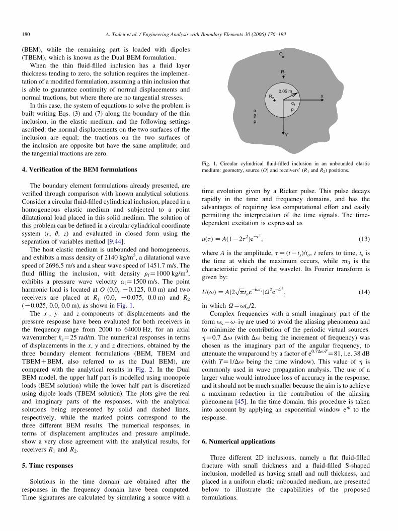
Fig. 1. Circular cylindrical fluid-filled inclusion in an unbounded elastic
medium: geometry, source (O) and receivers’ (R1 and R2) positions.
A. Tadeu et al. / Engineering Analysis with Boundary Elements 30 (2006) 176–193180
(BEM), while the remaining part is loaded with dipoles
(TBEM), which is known as the Dual BEM formulation.
When the thin fluid-filled inclusion has a fluid layer
thickness tending to zero, the solution requires the implemen-
tation of a modified formulation, assuming a thin inclusion that
is able to guarantee continuity of normal displacements and
normal tractions, but where there are no tangential stresses.
In this case, the system of equations to solve the problem is
built writing Eqs. (3) and (7) along the boundary of the thin
inclusion, in the elastic medium, and the following settings
ascribed: the normal displacements on the two surfaces of the
inclusion are equal; the tractions on the two surfaces of
the inclusion are opposite but have the same amplitude; and
the tangential tractions are zero.
4. Verification of the BEM formulations
The boundary element formulations already presented, are
verified through comparison with known analytical solutions.
Consider a circular fluid-filled cylindrical inclusion, placed in a
homogeneous elastic medium and subjected to a point
dilatational load placed in this solid medium. The solution of
this problem can be defined in a circular cylindrical coordinate
system (r, q, z) and evaluated in closed form using the
separation of variables method [9,44].
The host elastic medium is unbounded and homogeneous,
and exhibits a mass density of 2140 kg/m3, a dilatational wave
speed of 2696.5 m/s and a shear wave speed of 1451.7 m/s. The
fluid filling the inclusion, with density rfZ1000 kg/m3,
exhibits a pressure wave velocity afZ1500 m/s. The point
harmonic load is located at O (0.0, K0.125, 0.0 m) and two
receivers are placed at R1 (0.0, K0.075, 0.0 m) and R2
(K0.025, 0.0, 0.0 m), as shown in Fig. 1.
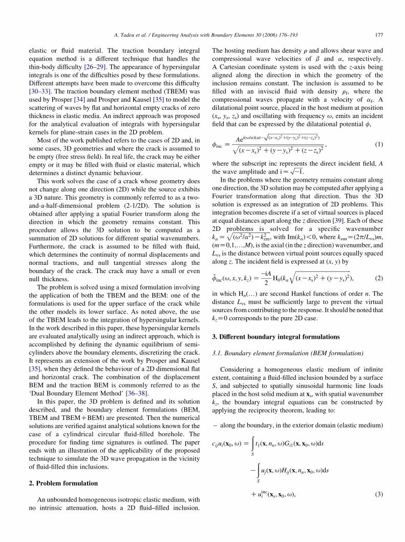
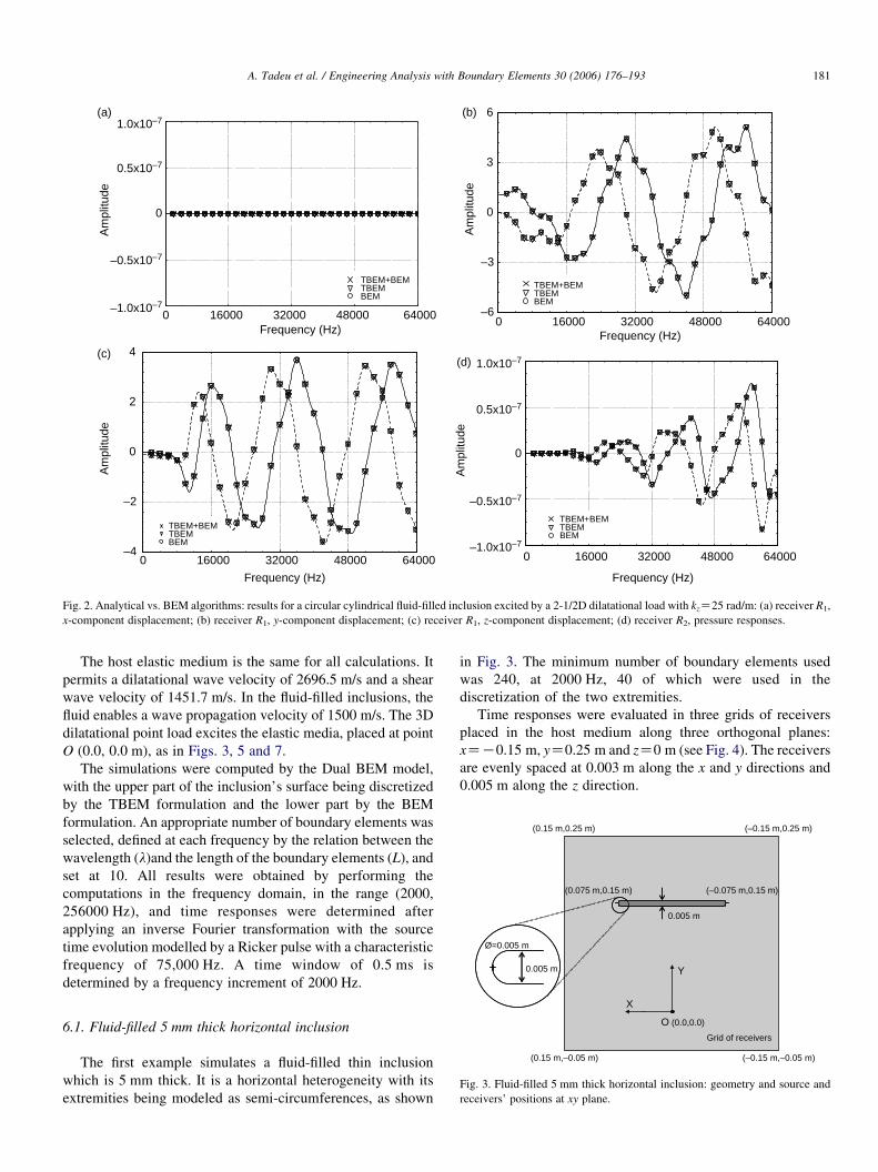
The x-, y- and z-components of displacements and the
pressure response have been evaluated for both receivers in
the frequency range from 2000 to 64000 Hz, for an axial
wavenumber kzZ25 rad/m. The numerical responses in terms
of displacements in the x, y and z directions, obtained by the
three boundary element formulations (BEM, TBEM and
TBEMCBEM, also referred to as the Dual BEM), are
compared with the analytical results in Fig. 2. In the Dual
BEM model, the upper half part is modelled using monopole
loads (BEM solution) while the lower half part is discretized
using dipole loads (TBEM solution). The plots give the real
and imaginary parts of the responses, with the analytical
solutions being represented by solid and dashed lines,
respectively, while the marked points correspond to the
three different BEM results. The numerical responses, in
terms of displacement amplitudes and pressure amplitude,
show a very close agreement with the analytical results, for
receivers R1 and R2.
5. Time responses
Solutions in the time domain are obtained after the
responses in the frequency domain have been computed.
Time signatures are calculated by simulating a source with a
time evolution given by a Ricker pulse. This pulse decays
rapidly in the time and frequency domains, and has the
advantages of requiring less computational effort and easily
permitting the interpretation of the time signals. The time-
dependent excitation is expressed as
uðtÞ Z Að1K2t2ÞeKt2
; (13)
where A is the amplitude, tZ ðtKtsÞ=to, t refers to time, ts is
the time at which the maximum occurs, while pt0 is the
characteristic period of the wavelet. Its Fourier transform is
given by:
UðuÞ Z A½2ffiffiffiffip
ptoeKiuts�U2eKU2
; (14)
in which UZuto/2.
Complex frequencies with a small imaginary part of the
form ucZu–ih are used to avoid the aliasing phenomena and
to minimize the contribution of the periodic virtual sources.
hZ0.7 Du (with Du being the increment of frequency) was
chosen as the imaginary part of the angular frequency, to
attenuate the wraparound by a factor of e0.7DuTZ81, i.e. 38 dB
(with TZ1/Du being the time window). This value of h is
commonly used in wave propagation analysis. The use of a
larger value would introduce loss of accuracy in the response,
and it should not be much smaller because the aim is to achieve
a maximum reduction in the contribution of the aliasing
phenomena [45]. In the time domain, this procedure is taken
into account by applying an exponential window eht to the
response.
6. Numerical applications
Three different 2D inclusions, namely a flat fluid-filled
fracture with small thickness and a fluid-filled S-shaped
inclusion, modelled as having small and null thickness, and
placed in a uniform elastic unbounded medium, are presented
below to illustrate the capabilities of the proposed
formulations.
–0.5x10⁻⁷
0
(a) (b)
(c)(d)
0.5x10⁻⁷
1.0x10⁻⁷
–1.0x10–70 16000 32000 48000 64000
TBEM+BEMTBEMBEM
Frequency (Hz)0 16000 32000 48000 64000
Frequency (Hz)
0 16000 32000 48000 64000
Frequency (Hz)
Am
plitu
de
–0.5x10⁻⁷
0
0.5x10⁻⁷
1.0x10⁻⁷
–1.0x10⁻⁷
0 16000 32000 48000 64000
Frequency (Hz)
Am
plitu
de
–6
–3
0
3
6
Am
plitu
de
–4
–2
0
2
4
Am
plitu
de
TBEM+BEMTBEMBEM
TBEM+BEMTBEMBEM
TBEM+BEMTBEMBEM
Fig. 2. Analytical vs. BEM algorithms: results for a circular cylindrical fluid-filled inclusion excited by a 2-1/2D dilatational load with kzZ25 rad/m: (a) receiver R1,
x-component displacement; (b) receiver R1, y-component displacement; (c) receiver R1, z-component displacement; (d) receiver R2, pressure responses.
Y0.005 m
(0.15 m,0.25 m) (–0.15 m,0.25 m)
Ø=0.005 m
(0.075 m,0.15 m) (–0.075 m,0.15 m)
0.005 m
A. Tadeu et al. / Engineering Analysis with Boundary Elements 30 (2006) 176–193 181
The host elastic medium is the same for all calculations. It
permits a dilatational wave velocity of 2696.5 m/s and a shear
wave velocity of 1451.7 m/s. In the fluid-filled inclusions, the
fluid enables a wave propagation velocity of 1500 m/s. The 3D
dilatational point load excites the elastic media, placed at point
O (0.0, 0.0 m), as in Figs. 3, 5 and 7.
The simulations were computed by the Dual BEM model,
with the upper part of the inclusion’s surface being discretized
by the TBEM formulation and the lower part by the BEM
formulation. An appropriate number of boundary elements was
selected, defined at each frequency by the relation between the
wavelength (l)and the length of the boundary elements (L), and
set at 10. All results were obtained by performing the
computations in the frequency domain, in the range (2000,
256000 Hz), and time responses were determined after
applying an inverse Fourier transformation with the source
time evolution modelled by a Ricker pulse with a characteristic
frequency of 75,000 Hz. A time window of 0.5 ms is
determined by a frequency increment of 2000 Hz.
X
O (0.0,0.0)
Grid of receivers
(–0.15 m,–0.05 m)(0.15 m,–0.05 m)
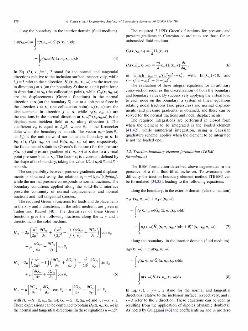
Fig. 3. Fluid-filled 5 mm thick horizontal inclusion: geometry and source and
receivers’ positions at xy plane.
6.1. Fluid-filled 5 mm thick horizontal inclusion
The first example simulates a fluid-filled thin inclusion
which is 5 mm thick. It is a horizontal heterogeneity with its
extremities being modeled as semi-circumferences, as shown
in Fig. 3. The minimum number of boundary elements used
was 240, at 2000 Hz, 40 of which were used in the
discretization of the two extremities.
Time responses were evaluated in three grids of receivers
placed in the host medium along three orthogonal planes:
xZK0.15 m, yZ0.25 m and zZ0 m (see Fig. 4). The receivers
are evenly spaced at 0.003 m along the x and y directions and
0.005 m along the z direction.
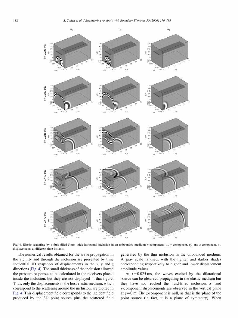
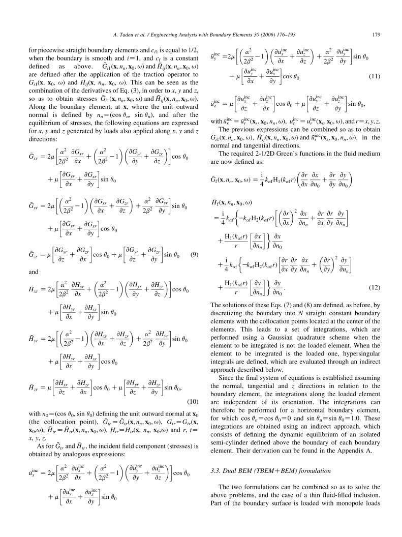
Fig. 4. Elastic scattering by a fluid-filled 5 mm thick horizontal inclusion in an unbounded medium: x-component, ux, y-component, uy, and z-component, uz,
displacements at different time instants.
A. Tadeu et al. / Engineering Analysis with Boundary Elements 30 (2006) 176–193182
The numerical results obtained for the wave propagation in
the vicinity and through the inclusion are presented by time
sequential 3D snapshots of displacements in the x, y and z
directions (Fig. 4). The small thickness of the inclusion allowed
the pressure responses to be calculated in the receivers placed
inside the inclusion, but they are not displayed in that figure.
Thus, only the displacements in the host elastic medium, which
correspond to the scattering around the inclusion, are plotted in
Fig. 4. This displacement field corresponds to the incident field
produced by the 3D point source plus the scattered field
generated by the thin inclusion in the unbounded medium.
A gray scale is used, with the lighter and darker shades
corresponding respectively to higher and lower displacement
amplitude values.
At tZ0.025 ms, the waves excited by the dilatational
source can be observed propagating in the elastic medium but
they have not reached the fluid-filled inclusion. x- and
y-component displacements are observed in the vertical plane
at zZ0 m. The z-component is null, as that is the plane of the
point source (in fact, it is a plane of symmetry). When
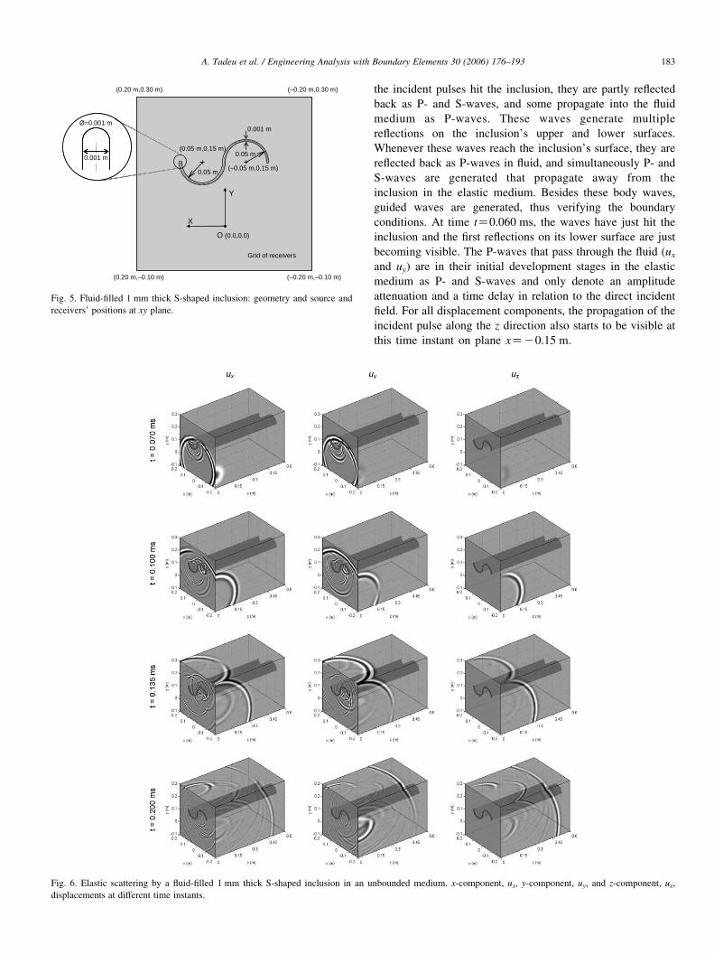
Fig. 6. Elastic scattering by a fluid-filled 1 mm thick S-shaped inclusion in an u
displacements at different time instants.
O (0.0,0.0)
X
Y
O (0.0,0.0)
X
Y
Grid of receivers
(0.20 m,0.30 m) (–0.20 m,0.30 m)
(0.20 m,–0.10 m) (–0.20 m,–0.10 m)
Ø=0.001 m
0.001 m
0.001 m
0.05 m
0.05 m(–0.05 m,0.15 m)
(0.05 m,0.15 m)
Fig. 5. Fluid-filled 1 mm thick S-shaped inclusion: geometry and source and
receivers’ positions at xy plane.
A. Tadeu et al. / Engineering Analysis with Boundary Elements 30 (2006) 176–193 183
the incident pulses hit the inclusion, they are partly reflected
back as P- and S-waves, and some propagate into the fluid
medium as P-waves. These waves generate multiple
reflections on the inclusion’s upper and lower surfaces.
Whenever these waves reach the inclusion’s surface, they are
reflected back as P-waves in fluid, and simultaneously P- and
S-waves are generated that propagate away from the
inclusion in the elastic medium. Besides these body waves,
guided waves are generated, thus verifying the boundary
conditions. At time tZ0.060 ms, the waves have just hit the
inclusion and the first reflections on its lower surface are just
becoming visible. The P-waves that pass through the fluid (ux
and uy) are in their initial development stages in the elastic
medium as P- and S-waves and only denote an amplitude
attenuation and a time delay in relation to the direct incident
field. For all displacement components, the propagation of the
incident pulse along the z direction also starts to be visible at
this time instant on plane xZK0.15 m.
nbounded medium. x-component, ux, y-component, uy, and z-component, uz,
O (0.0,0.0)
X
Y
(0.20 m,0.30 m) (–0.20 m,0.30 m)
(0.20 m,–0.10 m) (–0.20 m,–0.10 m)
Grid of receivers
0.05 m
0.05 m (–0.05 m,0.15 m)
(0.05 m,0.15 m)
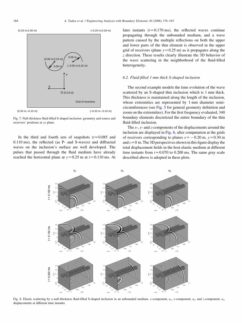
Fig. 7. Null-thickness fluid-filled S-shaped inclusion: geometry and source and
receivers’ positions at xy plane.
A. Tadeu et al. / Engineering Analysis with Boundary Elements 30 (2006) 176–193184
In the third and fourth sets of snapshots (tZ0.085 and
0.110 ms), the reflected (as P- and S-waves) and diffracted
waves on the inclusion’s surface are well developed. The
pulses that passed through the fluid medium have already
reached the horizontal plane at yZ0.25 m at tZ0.110 ms. At
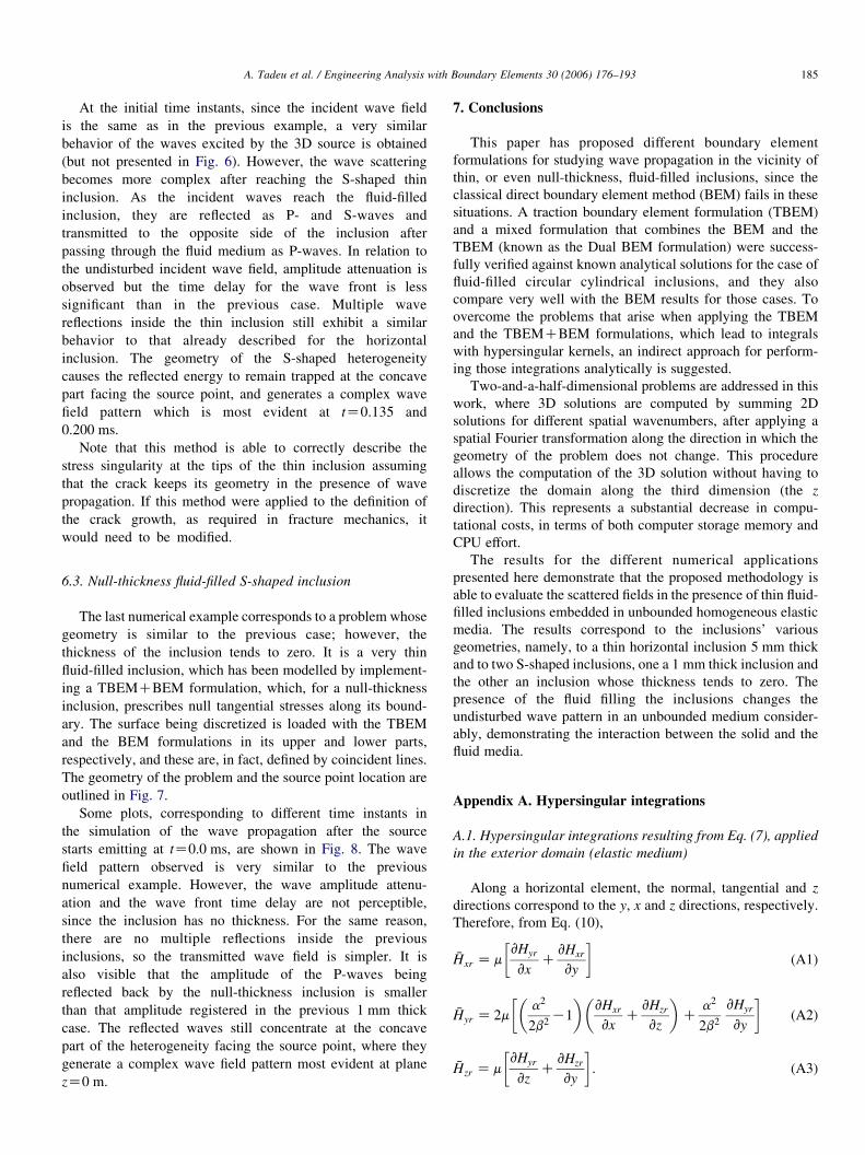
Fig. 8. Elastic scattering by a null-thickness fluid-filled S-shaped inclusion in an
displacements at different time instants.
later instants (tZ0.170 ms), the reflected waves continue
propagating through the unbounded medium, and a wave
pattern caused by the multiple reflections on both the upper
and lower parts of the thin element is observed in the upper
grid of receivers (plane yZ0.25 m) as it propagates along the
z direction. These results clearly illustrate the 3D behavior of
the wave scattering in the neighborhood of the fluid-filled
heterogeneity.
6.2. Fluid-filled 1 mm thick S-shaped inclusion
The second example models the time evolution of the wave
scattered by an S-shaped thin inclusion which is 1 mm thick.
This thickness is maintained along the length of the inclusion,
whose extremities are represented by 1 mm diameter semi-
circumferences (see Fig. 5 for general geometry definition and
zoom on the extremities). For the first frequency evaluated, 340
boundary elements discretized the entire boundary of the thin
fluid-filled inclusion.
The x-, y- and z-components of the displacements around the
inclusion are displayed in Fig. 6, after computation at the grids
of receivers corresponding to planes xZK0.20 m, yZ0.30 m
and zZ0 m. The 3D perspectives shown in this figure display the
total displacement fields in the host elastic medium at different
time instants from tZ0.070 to 0.200 ms. The same gray scale
described above is adopted in these plots.
unbounded medium. x-component, ux, y-component, uy, and z-component, uz,
A. Tadeu et al. / Engineering Analysis with Boundary Elements 30 (2006) 176–193 185
At the initial time instants, since the incident wave field
is the same as in the previous example, a very similar
behavior of the waves excited by the 3D source is obtained
(but not presented in Fig. 6). However, the wave scattering
becomes more complex after reaching the S-shaped thin
inclusion. As the incident waves reach the fluid-filled
inclusion, they are reflected as P- and S-waves and
transmitted to the opposite side of the inclusion after
passing through the fluid medium as P-waves. In relation to
the undisturbed incident wave field, amplitude attenuation is
observed but the time delay for the wave front is less
significant than in the previous case. Multiple wave
reflections inside the thin inclusion still exhibit a similar
behavior to that already described for the horizontal
inclusion. The geometry of the S-shaped heterogeneity
causes the reflected energy to remain trapped at the concave
part facing the source point, and generates a complex wave
field pattern which is most evident at tZ0.135 and
0.200 ms.
Note that this method is able to correctly describe the
stress singularity at the tips of the thin inclusion assuming
that the crack keeps its geometry in the presence of wave
propagation. If this method were applied to the definition of
the crack growth, as required in fracture mechanics, it
would need to be modified.
6.3. Null-thickness fluid-filled S-shaped inclusion
The last numerical example corresponds to a problem whose
geometry is similar to the previous case; however, the
thickness of the inclusion tends to zero. It is a very thin
fluid-filled inclusion, which has been modelled by implement-
ing a TBEMCBEM formulation, which, for a null-thickness
inclusion, prescribes null tangential stresses along its bound-
ary. The surface being discretized is loaded with the TBEM
and the BEM formulations in its upper and lower parts,
respectively, and these are, in fact, defined by coincident lines.
The geometry of the problem and the source point location are
outlined in Fig. 7.
Some plots, corresponding to different time instants in
the simulation of the wave propagation after the source
starts emitting at tZ0.0 ms, are shown in Fig. 8. The wave
field pattern observed is very similar to the previous
numerical example. However, the wave amplitude attenu-
ation and the wave front time delay are not perceptible,
since the inclusion has no thickness. For the same reason,
there are no multiple reflections inside the previous
inclusions, so the transmitted wave field is simpler. It is
also visible that the amplitude of the P-waves being
reflected back by the null-thickness inclusion is smaller
than that amplitude registered in the previous 1 mm thick
case. The reflected waves still concentrate at the concave
part of the heterogeneity facing the source point, where they
generate a complex wave field pattern most evident at plane
zZ0 m.
7. Conclusions
This paper has proposed different boundary element
formulations for studying wave propagation in the vicinity of
thin, or even null-thickness, fluid-filled inclusions, since the
classical direct boundary element method (BEM) fails in these
situations. A traction boundary element formulation (TBEM)
and a mixed formulation that combines the BEM and the
TBEM (known as the Dual BEM formulation) were success-
fully verified against known analytical solutions for the case of
fluid-filled circular cylindrical inclusions, and they also
compare very well with the BEM results for those cases. To
overcome the problems that arise when applying the TBEM
and the TBEMCBEM formulations, which lead to integrals
with hypersingular kernels, an indirect approach for perform-
ing those integrations analytically is suggested.
Two-and-a-half-dimensional problems are addressed in this
work, where 3D solutions are computed by summing 2D
solutions for different spatial wavenumbers, after applying a
spatial Fourier transformation along the direction in which the
geometry of the problem does not change. This procedure
allows the computation of the 3D solution without having to
discretize the domain along the third dimension (the z
direction). This represents a substantial decrease in compu-
tational costs, in terms of both computer storage memory and
CPU effort.
The results for the different numerical applications
presented here demonstrate that the proposed methodology is
able to evaluate the scattered fields in the presence of thin fluid-
filled inclusions embedded in unbounded homogeneous elastic
media. The results correspond to the inclusions’ various
geometries, namely, to a thin horizontal inclusion 5 mm thick
and to two S-shaped inclusions, one a 1 mm thick inclusion and
the other an inclusion whose thickness tends to zero. The
presence of the fluid filling the inclusions changes the
undisturbed wave pattern in an unbounded medium consider-
ably, demonstrating the interaction between the solid and the
fluid media.
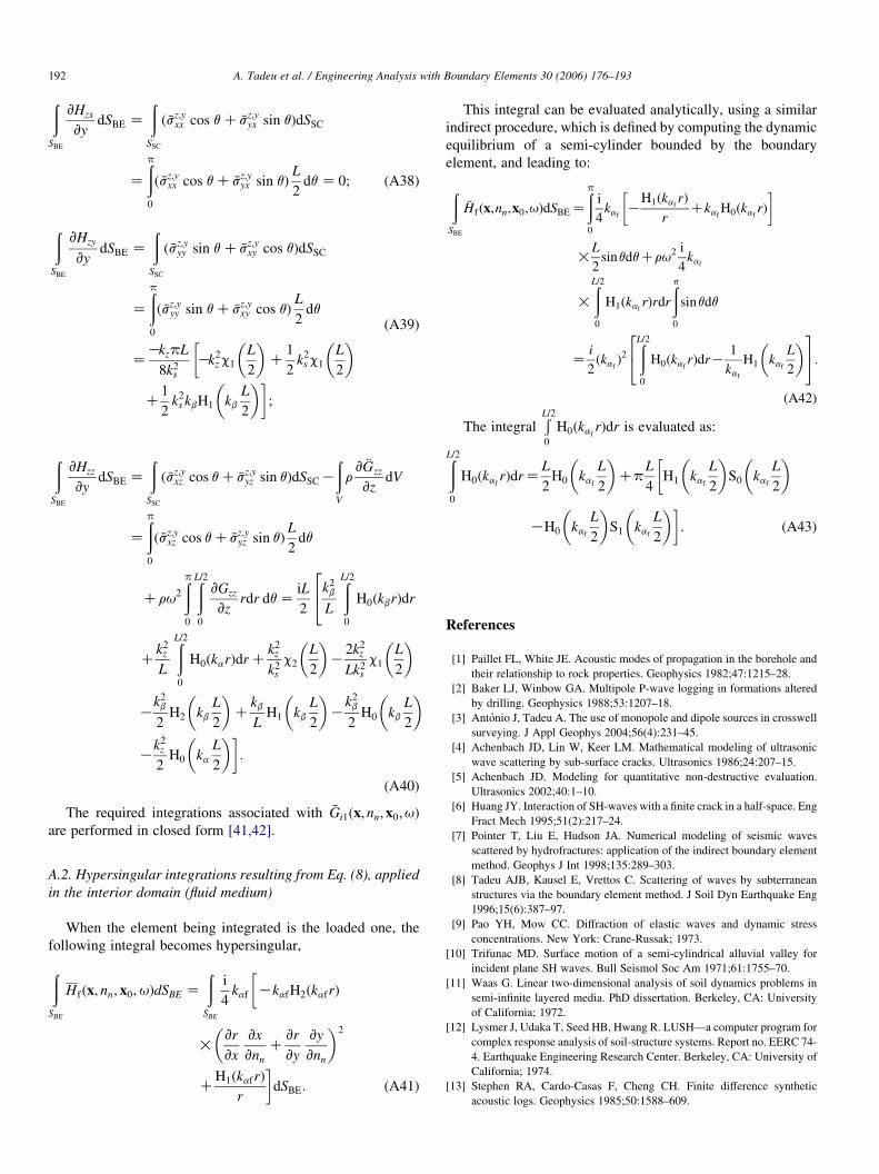
Appendix A. Hypersingular integrations
A.1. Hypersingular integrations resulting from Eq. (7), applied
in the exterior domain (elastic medium)
Along a horizontal element, the normal, tangential and z
directions correspond to the y, x and z directions, respectively.
Therefore, from Eq. (10),
�Hxr Z mvHyr
vxC
vHxr
vy
� �(A1)
�Hyr Z 2ma2
2b2K1
� �vHxr
vxC
vHzr
vz
� �C
a2
2b2
vHyr
vy
� �(A2)
�Hzr Z mvHyr
vzC
vHzr
vy
� �: (A3)
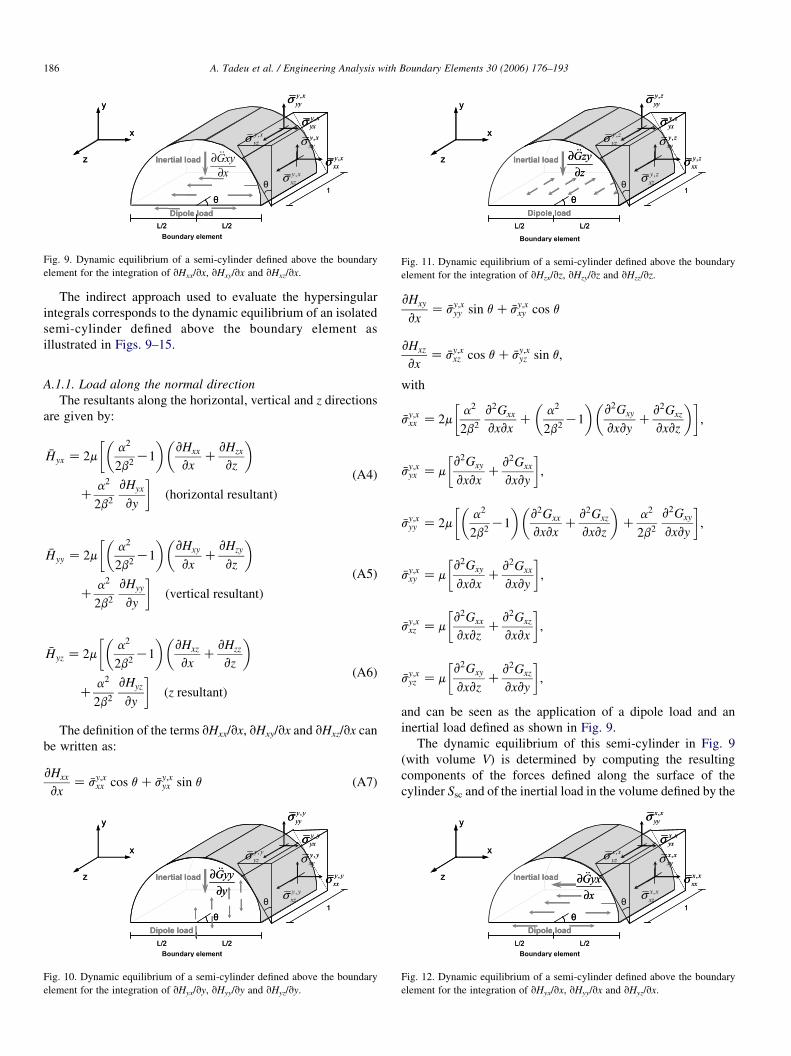
Fig. 9. Dynamic equilibrium of a semi-cylinder defined above the boundary
element for the integration of vHxx/vx, vHxy/vx and vHxz/vx.Fig. 11. Dynamic equilibrium of a semi-cylinder defined above the boundary
element for the integration of vHzx/vz, vHzy/vz and vHzz/vz.
A. Tadeu et al. / Engineering Analysis with Boundary Elements 30 (2006) 176–193186
The indirect approach used to evaluate the hypersingular
integrals corresponds to the dynamic equilibrium of an isolated
semi-cylinder defined above the boundary element as
illustrated in Figs. 9–15.
A.1.1. Load along the normal direction
The resultants along the horizontal, vertical and z directions
are given by:
�Hyx Z 2ma2
2b2K1
� �vHxx
vxC
vHzx
vz
� ��
Ca2
2b2
vHyx
vy
�ðhorizontal resultantÞ
(A4)
�Hyy Z 2ma2
2b2K1
� �vHxy
vxC
vHzy
vz
� ��
Ca2
2b2
vHyy
vy
�ðvertical resultantÞ
(A5)
�Hyz Z 2ma2
2b2K1
� �vHxz
vxC
vHzz
vz
� ��
Ca2
2b2
vHyz
vy
�ðz resultantÞ
(A6)
The definition of the terms vHxx/vx, vHxy/vx and vHxz/vx can
be written as:
vHxx
vxZ �sy;x
xx cos q C �sy;xyx sin q (A7)
Fig. 10. Dynamic equilibrium of a semi-cylinder defined above the boundary
element for the integration of vHyx/vy, vHyy/vy and vHyz/vy.
vHxy
vxZ �sy;x
yy sin q C �sy;xxy cos q
vHxz
vxZ �sy;x
xz cos q C �sy;xyz sin q;
with
�sy;xxx Z 2m
a2
2b2
v2Gxx
vxvxC
a2
2b2K1
� �v2Gxy
vxvyC
v2Gxz
vxvz
� �� �;
�sy;xyx Z m
v2Gxy
vxvxC
v2Gxx
vxvy
� �;
�sy;xyy Z 2m
a2
2b2K1
� �v2Gxx
vxvxC
v2Gxz
vxvz
� �C
a2
2b2
v2Gxy
vxvy
� �;
�sy;xxy Z m
v2Gxy
vxvxC
v2Gxx
vxvy
� �;
�sy;xxz Z m
v2Gxx
vxvzC
v2Gxz
vxvx
� �;
�sy;xyz Z m
v2Gxy
vxvzC
v2Gxz
vxvy
� �;
and can be seen as the application of a dipole load and an
inertial load defined as shown in Fig. 9.
The dynamic equilibrium of this semi-cylinder in Fig. 9
(with volume V) is determined by computing the resulting
components of the forces defined along the surface of the
cylinder Ssc and of the inertial load in the volume defined by the
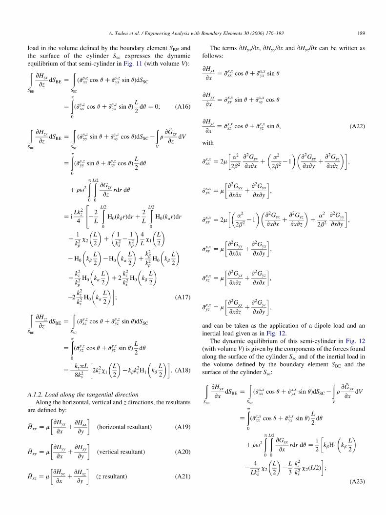
Fig. 12. Dynamic equilibrium of a semi-cylinder defined above the boundary
element for the integration of vHyx/vx, vHyy/vx and vHyz/vx.
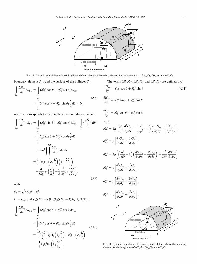
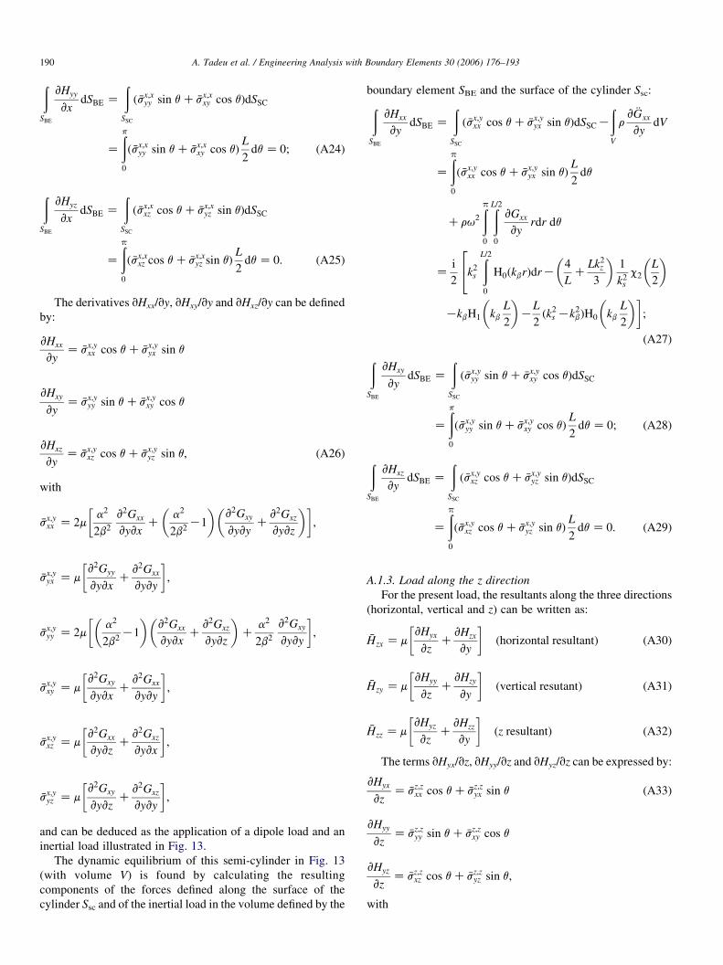
Fig. 13. Dynamic equilibrium of a semi-cylinder defined above the boundary element for the integration of vHxx/vy, vHxy/vy and vHxz/vy.
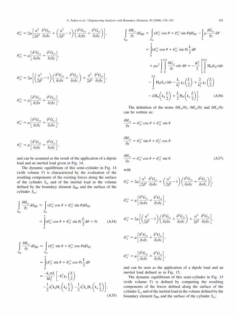
Fig. 14. Dynamic equilibrium of a semi-cylinder defined above the boundary
element for the integration of vHyx/vz, vHyy/vz and vHyz/vz.
A. Tadeu et al. / Engineering Analysis with Boundary Elements 30 (2006) 176–193 187
boundary element SBE and the surface of the cylinder Ssc:ðSBE
vHxx
vxdSBE Z
ðSSC
ð �sy;xxx cos q C �sy;x
yx sin qÞdSSC
Z
ðp
0
ð �sy;xxx cos q C �sy;x
yx sin qÞL
2dq Z 0;
(A8)
where L corresponds to the length of the boundary element;
ðSBE
vHxy
vxdSBE Z
ðSSC
ð �sy;xyy sin q C �sy;x
xy cos qÞdSSCK
ðV
rv €Gxy
vxdV
Z
ðp
0
ð �sy;xyy sin q C �sy;x
xy cos qÞL
2dq
Cru2
ðp
0
ðL=2
0
vGxy
vxrdr dq
Zi
2kaH1 ka
L
2
� �1K
2b2
a2
� ��
K4
Lk2s
c2
L
2
� �K
L
3
k2z
k2s
c2
L
2
� ��;
(A9)
with
kb Zffiffiffiffiffiffiffiffiffiffiffiffiffiffiffiffiffiffiffiffiffiu2=b2Kk2
z
q;
ks Z u=b and cnðL=2Þ Z knbHnðkbðL=2ÞÞKkn
aHnðkaðL=2ÞÞ;
ðSBE
vHxz
vxdSBE Z
ðSSC
ð �sy;xxz cos q C �sy;x
yz sin qÞdSSC
Z
ðp
0
ð �sy;xxz cos q C �sy;x
yz sin qÞL
2dq
ZKkzpL
8k2s
k3bH1 kb
L
2
� �Kk3
aH1 ka
L
2
� ��
K1
2kbk2
s H1 kb
L
2
� ��:
(A10)
The terms vHyx/vy, vHyy/vy and vHyz/vy are defined by:
vHyx
vyZ �sy;y
xx cos q C �sy;yyx sin q (A11)
vHyy
vyZ �sy;y
yy sin q C �sy;yxy cos q
vHyz
vyZ �sy;y
xz cos q C �sy;yyz sin q;
with
�sy;yxx Z 2m
a2
2b2
v2Gyx
vyvxC
a2
2b2K1
� �v2Gyy
vyvyC
v2Gyz
vyvz
� �� �;
�sy;yyx Z m
v2Gyy
vyvxC
v2Gyx
vyvy
� �;
�sy;yyy Z 2m
a2
2b2K1
� �v2Gyx
vyvxC
v2Gyz
vyvz
� �C
a2
2b2
v2Gyy
vyvy
� �;
�sy;yxy Z m
v2Gyy
vyvxC
v2Gyx
vyvy
� �;
�sy;yxz Z m
v2Gyx
vyvzC
v2Gyz
vyvx
� �;
�sy;yyz Z m
v2Gyy
vyvzC
v2Gyz
vyvy
� �;
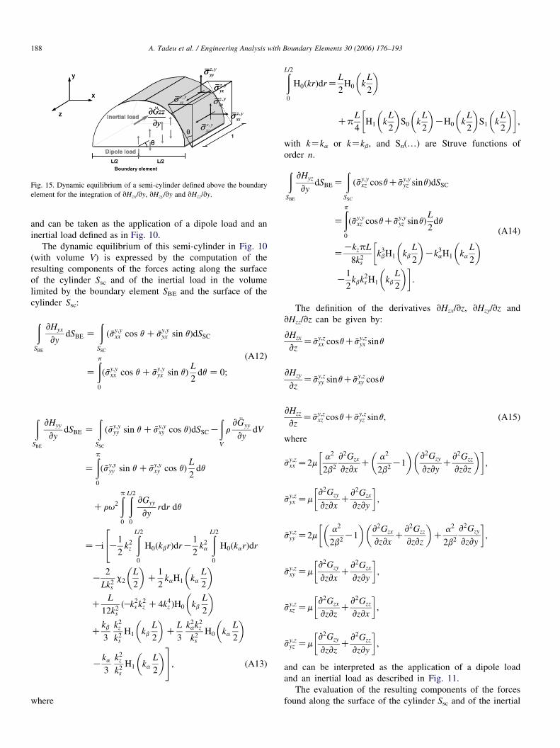
Fig. 15. Dynamic equilibrium of a semi-cylinder defined above the boundary
element for the integration of vHzx/vy, vHzy/vy and vHzz/vy.
A. Tadeu et al. / Engineering Analysis with Boundary Elements 30 (2006) 176–193188
and can be taken as the application of a dipole load and an
inertial load defined as in Fig. 10.
The dynamic equilibrium of this semi-cylinder in Fig. 10
(with volume V) is expressed by the computation of the
resulting components of the forces acting along the surface
of the cylinder Ssc and of the inertial load in the volume
limited by the boundary element SBE and the surface of the
cylinder Ssc:
ðSBE
vHyx
vydSBE Z
ðSSC
ð �sy;yxx cos q C �sy;y
yx sin qÞdSSC
Z
ðp
0
ð �sy;yxx cos q C �sy;y
yx sin qÞL
2dq Z 0;
(A12)
ðSBE
vHyy
vydSBE Z
ðSSC
ð �sy;yyy sin q C �sy;y
xy cos qÞdSSCK
ðV
rv €Gyy
vydV
Z
ðp
0
ð �sy;yyy sin q C �sy;y
xy cos qÞL
2dq
Cru2
ðp
0
ðL=2
0
vGyy
vyrdr dq
ZKi K1
2k2
z
ðL=2
0
H0ðkbrÞdrK1
2k2
a
ðL=2
0
H0ðkarÞdr
24
K2
Lk2s
c2
L
2
� �C
1
2kaH1 ka
L
2
� �
CL
12k2s
ðKk2s k2
z C4k4z ÞH0 kb
L
2
� �
Ckb
3
k2z
k2s
H1 kb
L
2
� �C
L
3
k2ak2
z
k2s
H0 ka
L
2
� �
Kka
3
k2z
k2s
H1 ka
L
2
� �35; ðA13Þ
where
ðL=2
0
H0ðkrÞdrZL
2H0 k
L
2
� �
CpL
4H1 k
L
2
� �S0 k
L
2
� �KH0 k
L
2
� �S1 k
L
2
� �� �;
with kZka or kZkb, and Sn(.) are Struve functions of
order n.
ðSBE
vHyz
vydSBE Z
ðSSC
ð �sy;yxz cosqC �sy;y
yz sinqÞdSSC
Z
ðp
0
ð �sy;yxz cosqC �sy;y
yz sinqÞL
2dq
ZKkzpL
8k2s
k3bH1 kb
L
2
� �Kk3
aH1 ka
L
2
� ��
K1
2kbk2
s H1 kb
L
2
� ��:
(A14)
The definition of the derivatives vHzx/vz, vHzy/vz and
vHzz/vz can be given by:
vHzx
vzZ �sy;z
xx cosqC �sy;zyx sinq
vHzy
vzZ �sy;z
yy sinqC �sy;zxy cosq
vHzz
vzZ �sy;z
xz cosqC �sy;zyz sinq; (A15)
where
�sy;zxx Z2m
a2
2b2
v2Gzx
vzvxC
a2
2b2K1
� �v2Gzy
vzvyC
v2Gzz
vzvz
� �� �;
�sy;zyx Zm
v2Gzy
vzvxC
v2Gzx
vzvy
� �;
�sy;zyy Z2m
a2
2b2K1
� �v2Gzx
vzvxC
v2Gzz
vzvz
� �C
a2
2b2
v2Gzy
vzvy
� �;
�sy;zxy Zm
v2Gzy
vzvxC
v2Gzx
vzvy
� �;
�sy;zxz Zm
v2Gzx
vzvzC
v2Gzz
vzvx
� �;
�sy;zyz Zm
v2Gzy
vzvzC
v2Gzz
vzvy
� �;
and can be interpreted as the application of a dipole load
and an inertial load as described in Fig. 11.
The evaluation of the resulting components of the forces
found along the surface of the cylinder Ssc and of the inertial
A. Tadeu et al. / Engineering Analysis with Boundary Elements 30 (2006) 176–193 189
load in the volume defined by the boundary element SBE and
the surface of the cylinder Ssc expresses the dynamic
equilibrium of that semi-cylinder in Fig. 11 (with volume V):ðSBE
vHzx
vzdSBE Z
ðSSC
ð �sy;zxx cos q C �sy;z
yx sin qÞdSSC
Z
ðp
0
ð �sy;zxx cos q C �sy;z
yx sin qÞL
2dq Z 0; ðA16)
ðSBE
vHzy
vzdSBE Z
ðSSC
ð �sy;zyy sin q C �sy;z
xy cos qÞdSSC K
ðV
rv €Gzy
vzdV
Z
ðp
0
ð �sy;zyy sin q C �sy;z
xy cos qÞL
2dq
Cru2
ðp
0
ðL=2
0
vGzy
vzrdr dq
Z iLk2
z
4K
2
L
ðL=2
0
H0ðkbrÞdr C2
L
ðL=2
0
H0ðkarÞdr
24
C1
k2p
c2
L
2
� �C
1
k2s
K1
k2p
� �4
Lc1
L
2
� �
KH0 kb
L
2
� �KH0 ka
L
2
� �C
k2b
k2p
H0 kb
L
2
� �
Ck2
z
k2p
H0 ka
L
2
� �C2
k2z
k2s
H0 kb
L
2
� �
K2k2
z
k2s
H0 ka
L
2
� ��; ðA17)
ðSBE
vHzz
vzdSBE Z
ðSSC
ð �sy;zxz cos q C �sy;z
yz sin qÞdSSC
Z
ðp
0
ð �sy;zxz cos q C �sy;z
yz sin qÞL
2dq
ZKkzpL
8k2s
2k2z c1
L
2
� �Kkbk2
s H1 kb
L
2
� �� �: ðA18)
A.1.2. Load along the tangential direction
Along the horizontal, vertical and z directions, the resultants
are defined by:
�Hxx Z mvHyx
vxC
vHxx
vy
� �ðhorizontal resultantÞ (A19)
�Hxy Z mvHyy
vxC
vHxy
vy
� �ðvertical resultantÞ (A20)
�Hxz Z mvHyz
vxC
vHxz
vy
� �ðz resultantÞ (A21)
The terms vHyx/vx, vHyy/vx and vHyz/vx can be written as
follows:
vHyx
vxZ �sx;x
xx cos q C �sx;xyx sin q
vHyy
vxZ �sx;x
yy sin q C �sx;xxy cos q
vHyz
vxZ �sx;x
xz cos q C �sx;xyz sin q; (A22)
with
�sx;xxx Z 2m
a2
2b2
v2Gyx
vxvxC
a2
2b2K1
� �v2Gyy
vxvyC
v2Gyz
vxvz
� �� �;
�sx;xyx Z m
v2Gyy
vxvxC
v2Gyx
vxvy
� �;
�sx;xyy Z 2m
a2
2b2K1
� �v2Gyx
vxvxC
v2Gyz
vxvz
� �C
a2
2b2
v2Gyy
vxvy
� �;
�sx;xxy Z m
v2Gyy
vxvxC
v2Gyx
vxvy
� �;
�sx;xxz Z m
v2Gyx
vxvzC
v2Gyz
vxvx
� �;
�sx;xyz Z m
v2Gyy
vxvzC
v2Gyz
vxvy
� �;
and can be taken as the application of a dipole load and an
inertial load given as in Fig. 12.
The dynamic equilibrium of this semi-cylinder in Fig. 12
(with volume V) is given by the components of the forces found
along the surface of the cylinder Ssc and of the inertial load in
the volume defined by the boundary element SBE and the
surface of the cylinder Ssc:
ðSBE
vHyx
vxdSBE Z
ðSSC
ð �sx;xxx cos q C �sx;x
yx sin qÞdSSC K
ðV
rv €Gyx
vxdV
Z
ðp
0
ð �sx;xxx cos q C �sx;x
yx sin qÞL
2dq
Cru2
ðp
0
ðL=2
0
vGyx
vxrdr dq Z
i
2kbH1 kb
L
2
� ��
K4
Lk2s
c2
L
2
� �K
L
3
k2z
k2s
c2ðL=2Þ
�;
(A23)
A. Tadeu et al. / Engineering Analysis with Boundary Elements 30 (2006) 176–193190
ðSBE
vHyy
vxdSBE Z
ðSSC
ð �sx;xyy sin q C �sx;x
xy cos qÞdSSC
Z
ðp
0
ð �sx;xyy sin q C �sx;x
xy cos qÞL
2dq Z 0; (A24)
ðSBE
vHyz
vxdSBE Z
ðSSC
ð �sx;xxz cos q C �sx;x
yz sin qÞdSSC
Z
ðp
0
ð �sx;xxz cos q C �sx;x
yz sin qÞL
2dq Z 0: (A25)
The derivatives vHxx/vy, vHxy/vy and vHxz/vy can be defined
by:
vHxx
vyZ �sx;y
xx cos q C �sx;yyx sin q
vHxy
vyZ �sx;y
yy sin q C �sx;yxy cos q
vHxz
vyZ �sx;y
xz cos q C �sx;yyz sin q; (A26)
with
�sx;yxx Z 2m
a2
2b2
v2Gxx
vyvxC
a2
2b2K1
� �v2Gxy
vyvyC
v2Gxz
vyvz
� �� �;
�sx;yyx Z m
v2Gyy
vyvxC
v2Gxx
vyvy
� �;
�sx;yyy Z 2m
a2
2b2K1
� �v2Gxx
vyvxC
v2Gxz
vyvz
� �C
a2
2b2
v2Gxy
vyvy
� �;
�sx;yxy Z m
v2Gxy
vyvxC
v2Gxx
vyvy
� �;
�sx;yxz Z m
v2Gxx
vyvzC
v2Gxz
vyvx
� �;
�sx;yyz Z m
v2Gxy
vyvzC
v2Gxz
vyvy
� �;
and can be deduced as the application of a dipole load and an
inertial load illustrated in Fig. 13.
The dynamic equilibrium of this semi-cylinder in Fig. 13
(with volume V) is found by calculating the resulting
components of the forces defined along the surface of the
cylinder Ssc and of the inertial load in the volume defined by the
boundary element SBE and the surface of the cylinder Ssc:ðSBE
vHxx
vydSBE Z
ðSSC
ð �sx;yxx cos q C �sx;y
yx sin qÞdSSC K
ðV
rv €Gxx
vydV
Z
ðp
0
ð �sx;yxx cos q C �sx;y
yx sin qÞL
2dq
Cru2
ðp
0
ðL=2
0
vGxx
vyrdr dq
Zi
2k2
s
ðL=2
0
H0ðkbrÞdrK4
LC
Lk2z
3
� �1
k2s
c2
L
2
� �24
KkbH1 kb
L
2
� �K
L
2ðk2
s Kk2bÞH0 kb
L
2
� ��;
(A27)
ðSBE
vHxy
vydSBE Z
ðSSC
ð �sx;yyy sin q C �sx;y
xy cos qÞdSSC
Z
ðp
0
ð �sx;yyy sin q C �sx;y
xy cos qÞL
2dq Z 0; (A28)
ðSBE
vHxz
vydSBE Z
ðSSC
ð �sx;yxz cos q C �sx;y
yz sin qÞdSSC
Z
ðp
0
ð �sx;yxz cos q C �sx;y
yz sin qÞL
2dq Z 0: (A29)
A.1.3. Load along the z direction
For the present load, the resultants along the three directions
(horizontal, vertical and z) can be written as:
�Hzx Z mvHyx
vzC
vHzx
vy
� �ðhorizontal resultantÞ (A30)
�Hzy Z mvHyy
vzC
vHzy
vy
� �ðvertical resutantÞ (A31)
�Hzz Z mvHyz
vzC
vHzz
vy
� �ðz resultantÞ (A32)
The terms vHyx/vz, vHyy/vz and vHyz/vz can be expressed by:
vHyx
vzZ �sz;z
xx cos q C �sz;zyx sin q (A33)
vHyy
vzZ �sz;z
yy sin q C �sz;zxy cos q
vHyz
vzZ �sz;z
xz cos q C �sz;zyz sin q;
with
A. Tadeu et al. / Engineering Analysis with Boundary Elements 30 (2006) 176–193 191
�sz;zxx Z 2m
a2
2b2
v2Gyx
vzvxC
a2
2b2K1
� �v2Gyy
vzvyC
v2Gyz
vzvz
� �� �;
�sz;zyx Z m
v2Gyy
vzvxC
v2Gyx
vzvy
� �;
�sz;zyy Z 2m
a2
2b2K1
� �v2Gyx
vzvxC
v2Gyz
vzvz
� �C
a2
2b2
v2Gyy
vzvy
� �;
�sz;zxy Z m
v2Gyy
vzvxC
v2Gyx
vzvy
� �;
�sz;zxz Z m
v2Gyx
vzvzC
v2Gyz
vzvx
� �;
�sz;zyz Z m
v2Gyy
vzvzC
v2Gyz
vzvy
� �;
and can be assumed as the result of the application of a dipole
load and an inertial load given in Fig. 14.
The dynamic equilibrium of this semi-cylinder in Fig. 14
(with volume V) is characterized by the evaluation of the
resulting components of the existing forces along the surface
of the cylinder Ssc and of the inertial load in the volume
defined by the boundary element SBE and the surface of the
cylinder Ssc:
ðSBE
vHyx
vzdSBE Z
ðSSC
ð �sz;zxx cos q C �sz;z
yx sin qÞdSSC
Z
ðp
0
ð �sz;zxx cos q C �sz;z
yx sin qÞL
2dq Z 0; (A34)
ðSBE
vHyy
vzdSBE Z
ðSSC
ð �sz;zyy sin q C �sz;z
xy cos qÞdSSC
Z
ðp
0
ð �sz;zyy sin q C �sz;z
xy cos qÞL
2dq
ZKkzpL
8k2s
Kk2z c1
L
2
� ��
K1
2k2
s kbH1 kb
L
2
� �K
1
2k2
s kaH1 ka
L
2
� ��;
(A35)
ðSBE
vHyz
vzdSBE Z
ðSSC
ð �sz;zxz cos q C �sz;z
yz sin qÞdSSCK
ðV
rv €Gyz
vzdV
Z
ðp
0
ð �sz;zxz cos q C �sz;z
yz sin qÞL
2dq
Cru2
ðp
0
ðL=2
0
vGyz
vzrdr dq ZK
ik2z
2
ðL=2
0
H0ðkbrÞdr
24
K
ðL=2
0
H0ðkarÞdrKL
k2s
c2
L
2
� �C
2
k2s
c1
L
2
� �
KLH0 kb
L
2
� �C
L
2H0 ka
L
2
� ��: (A36)
The definition of the terms vHzx/vy, vHzy/vy and vHzz/vy
can be written as:
vHzx
vyZ �sz;y
xx cos q C �sz;yyx sin q
vHzy
vyZ �sz;y
yy sin q C �sz;yxy cos q
vHzz
vyZ �sz;y
xz cos q C �sz;yyz sin q; (A37)
with
�sz;yxx Z 2m
a2
2b2
v2Gzx
vyvxC
a2
2b2K1
� �v2Gzy
vyvyC
v2Gzz
vyvz
� �� �;
�sz;yyx Z m
v2Gzy
vyvxC
v2Gzx
vyvy
� �;
�sz;yyy Z 2m
a2
2b2K1
� �v2Gzx
vyvxC
v2Gzz
vyvz
� �C
a2
2b2
v2Gzy
vyvy
� �;
�sz;yxz Z m
v2Gzx
vyvzC
v2Gzz
vyvx
� �;
�sz;yyz Z m
v2Gzy
vyvzC
v2Gzz
vyvy
� �;
and can be seen as the application of a dipole load and an
inertial load defined as in Fig. 15.
The dynamic equilibrium of this semi-cylinder in Fig. 15
(with volume V) is defined by computing the resulting
components of the forces defined along the surface of the
cylinder Ssc and of the inertial load in the volume defined by the
boundary element SBE and the surface of the cylinder Ssc:
A. Tadeu et al. / Engineering Analysis with Boundary Elements 30 (2006) 176–193192
ðSBE
vHzx
vydSBE Z
ðSSC
ð �sz;yxx cos q C �sz;y
yx sin qÞdSSC
Z
ðp
0
ð �sz;yxx cos q C �sz;y
yx sin qÞL
2dq Z 0; (A38)
ðSBE
vHzy
vydSBE Z
ðSSC
ð �sz;yyy sin q C �sz;y
xy cos qÞdSSC
Z
ðp
0
ð �sz;yyy sin q C �sz;y
xy cos qÞL
2dq
ZKkzpL
8k2s
Kk2z c1
L
2
� �C
1
2k2
s c1
L
2
� ��
C1
2k2
s kbH1 kb
L
2
� ��;
(A39)
ðSBE
vHzz
vydSBE Z
ðSSC
ð �sz;yxz cos q C �sz;y
yz sin qÞdSSCK
ðV
rv €Gzz
vzdV
Z
ðp
0
ð �sz;yxz cos q C �sz;y
yz sin qÞL
2dq
Cru2
ðp
0
ðL=2
0
vGzz
vzrdr dq Z
iL
2
k2b
L
ðL=2
0
H0ðkbrÞdr
24
Ck2
z
L
ðL=2
0
H0ðkarÞdr Ck2
z
k2s
c2
L
2
� �K
2k2z
Lk2s
c1
L
2
� �
Kk2
b
2H2 kb
L
2
� �C
kb
LH1 kb
L
2
� �K
k2b
2H0 kb
L
2
� �
Kk2
z
2H0 ka
L
2
� ��:
(A40)
The required integrations associated with �Gi1ðx;nn;x0;uÞ
are performed in closed form [41,42].
A.2. Hypersingular integrations resulting from Eq. (8), applied
in the interior domain (fluid medium)
When the element being integrated is the loaded one, the
following integral becomes hypersingular,
ðSBE
Hfðx; nn; x0;uÞdSBE Z
ðSBE
i
4kaf KkafH2ðkafrÞ
�
!vr
vx
vx
vnn
Cvr
vy
vy
vnn
� �2
CH1ðkafrÞ
r
�dSBE: (A41)
This integral can be evaluated analytically, using a similar
indirect procedure, which is defined by computing the dynamic
equilibrium of a semi-cylinder bounded by the boundary
element, and leading to:
ðSBE
�Hfðx;nn;x0;uÞdSBE Z
ðp
0
i
4kaf
KH1ðkaf
rÞ
rCkaf
H0ðkafrÞ
� �
!L
2sinqdqCru2 i
4kaf
!
ðL=2
0
H1ðkafrÞrdr
ðp
0
sinqdq
Zi
2ðkaf
Þ2ðL=2
0
H0ðkafrÞdrK
1
kaf
H1 kaf
L
2
� �24
35:
(A42)
The integralÐL=20
H0ðkafrÞdr is evaluated as:
ðL=2
0
H0ðkafrÞdrZ
L
2H0 kaf
L
2
� �Cp
L
4H1 kaf
L
2
� �S0 kaf
L
2
� ��
KH0 kaf
L
2
� �S1 kaf
L
2
� ��: (A43)
References
[1] Paillet FL, White JE. Acoustic modes of propagation in the borehole and
their relationship to rock properties. Geophysics 1982;47:1215–28.
[2] Baker LJ, Winbow GA. Multipole P-wave logging in formations altered
by drilling. Geophysics 1988;53:1207–18.
[3] Antonio J, Tadeu A. The use of monopole and dipole sources in crosswell
surveying. J Appl Geophys 2004;56(4):231–45.
[4] Achenbach JD, Lin W, Keer LM. Mathematical modeling of ultrasonic
wave scattering by sub-surface cracks. Ultrasonics 1986;24:207–15.
[5] Achenbach JD. Modeling for quantitative non-destructive evaluation.
Ultrasonics 2002;40:1–10.
[6] Huang JY. Interaction of SH-waves with a finite crack in a half-space. Eng
Fract Mech 1995;51(2):217–24.
[7] Pointer T, Liu E, Hudson JA. Numerical modeling of seismic waves
scattered by hydrofractures: application of the indirect boundary element
method. Geophys J Int 1998;135:289–303.
[8] Tadeu AJB, Kausel E, Vrettos C. Scattering of waves by subterranean
structures via the boundary element method. J Soil Dyn Earthquake Eng
1996;15(6):387–97.
[9] Pao YH, Mow CC. Diffraction of elastic waves and dynamic stress
concentrations. New York: Crane-Russak; 1973.
[10] Trifunac MD. Surface motion of a semi-cylindrical alluvial valley for
incident plane SH waves. Bull Seismol Soc Am 1971;61:1755–70.
[11] Waas G. Linear two-dimensional analysis of soil dynamics problems in
semi-infinite layered media. PhD dissertation. Berkeley, CA: University
of California; 1972.
[12] Lysmer J, Udaka T, Seed HB, Hwang R. LUSH—a computer program for
complex response analysis of soil-structure systems. Report no. EERC 74-
4. Earthquake Engineering Research Center. Berkeley, CA: University of
California; 1974.
[13] Stephen RA, Cardo-Casas F, Cheng CH. Finite difference synthetic
acoustic logs. Geophysics 1985;50:1588–609.
A. Tadeu et al. / Engineering Analysis with Boundary Elements 30 (2006) 176–193 193
[14] Leslie HD, Randall CT. Multipole sources in boreholes penetrating
anisotropic formations: Numerical and experimental results. J Acoust Soc
Am 1992;91:12–27.
[15] Yoon KH. McMechan GA. 3-D finite difference modelling of elastic
waves in borehole environments. Geophysics 1992;57:793–804.
[16] Cheng N, Cheng CH, Toksoz MN. Borehole wave propagation in three
dimensions. J Acoust Soc Am 1995;97:3483–93.
[17] Ellefsen KJ. Elastic wave propagation along a borehole in an anisotropic
medium. PhD thesis. Cambridge, MA: MIT; 1990.
[18] Sinha BK, Norris AN, Chang SK. Borehole flexural modes in anisotropic
formations. 61st SEG Annual Meeting Expanded Abstracts, Houston;
1991.
[19] Norris AN, Sinha BK. Weak elastic anisotropy and the tube wave.
Geophysics 1983;58:1091–8.
[20] Bouchon M, Schmitt DP. Full wave acoustic logging in an irregular
borehole. Geophysics 1989;54:758–65.
[21] Bouchon M. A numerical simulation of the acoustic and elastic wavefields
radiated by a source in a fluid-filled borehole embedded in a layered
medium. Geophysics 1993;58:475–81.
[22] Dong W, Bouchon M, Toksoz MN. Borehole seismic-source radiation in
layered isotropic and anisotropic media: boundary element modelling.
Geophysics 1995;60:735–47.
[23] White JE, Sengbush RL. Shear waves from explosive sources. Geophysics
1963;28:1001–19.
[24] Ben-Menahem A, Kostek S. The equivalent force system of a monopole
source in a fluid-filled open borehole. Geophysics 1990;56:1477–81.
[25] De Hoop AT, De Hon BP, Kurkjian AL. Calculation of transient tube
wave signals in cross-borehole acoustics. J Acoust Soc Am 1994;95:
1773–89.
[26] Cruse TA. Boundary element analysis in computational fracture
mechanics. Dordrecht: Kluwer Academic; 1987.
[27] Sladek V, Sladek J. Transient elastodynamics three-dimensional
problems in cracked bodies. Appl Math Model 1984;8:2–10.
[28] Sladek V, Sladek J. A boundary integral equation method for dynamic
crack problems. Eng Fract Mech 1987;27(3):269–77.
[29] Takakuda K. Diffraction of plane harmonic waves by cracks. Bull JSME
1983;26(214):487–93.
[30] Rudolphi TJ. The use of simple solutions in the regularisation of
hypersingular boundary integral equations. Math Compnt Model 1991;15:
269–78.
[31] Lutz E, Ingraffea AR, Gray LJ. Use of ‘simple solutions’ for boundary
integral methods in elasticity and fracture analysis. Int J Numer Methods
Eng 1992;35:1737–51.
[32] Watson JO. Hermitian cubic boundary elements for plane problems of
fracture mechanics. Int J Struct Methods Mater Sci 1982;4:23–42.
[33] Watson JO. Singular boundary elements for the analysis of cracks in plane
strain. Int J Numer Methods Eng 1995;38:2389–411.
[34] Prosper D. Modeling and detection of delaminations in laminated plates.
PhD thesis. Cambridge: MIT; 2001.
[35] Prosper D, Kausel E. Wave scattering by cracks in laminated media. In:
Atluri SN, Nishioka T, Kikuchi M, editors. Proceedings advances in
computational engineering and sciences. Proceedings of the International
conference on computational engineering and science ICES’01. Tech
Science Press; 2001.
[36] Aliabadi MH. A new generation of boundary element methods in fracture
mechanics. Int J Fract 1997;86:91–125.
[37] Chen JT, Hong HK. Review of dual boundary element methods with
emphasis on hypersingular integrals and divergent series. Appl Mech Rev
1999;52:17–33.
[38] Aliabadi MH. The boundary element method. Application in solids and
structures, vol. 2. London: Wiley; 2002.
[39] Bouchon M, Aki K. Discrete wave-number representation of seismic-
source wave field. Bull Seism Soc Am 1977;67:259–77.
[40] Tadeu A, Kausel E. Green’s functions for two-and-a-half dimensional
elastodynamic problems. J Eng Mech ASCE 2000;126(10):1093–7.
[41] Tadeu A, Santos P, Kausel E. Closed-form integration of singular terms
for constant, linear and quadratic boundary elements—part I: SH wave
propagation. EABE Eng Anal Bound Elem 1999;23(8):671–81.
[42] Tadeu A, Santos P, Kausel E. Closed-form integration of singular terms
for constant, linear and quadratic boundary elements—part II: SV-P wave
propagation. EABE Eng Anal Bound Elem 1999;23(9):757–68.
[43] Guiggiani M. Formulation and numerical treatment of boundary integral
equations with hypersingular kernels Singular integrals in boundary
element methods. Southampton (UK) & Boston (USA): Computational
Mechanics Publications; 1998.
[44] Tadeu AJB. Modelling and seismic imaging of buried structures. PhD
thesis. Cambridge: MIT; 1992.
[45] Kausel E, Roesset JM. Frequency domain analysis of undamped systems.
J Eng Mech ASCE 1992;118(4):721–34.