3D Data, Phylogenetics, and Treesg562/PBDB2013/Day 5A - Phylogeny and trees.pdf... evidence for...

3D Data, Phylogenetics, and Trees

In this lecture…. 1.  Analysis of 3D landmarks 2.  Controversies about use of morphometrics in phylogene>cs 3.  Empirical data on phylogene>c component of morphometric varia>on 4.  Pros and cons of represen>ng morphometric data with trees 5.  Terminology of trees and phylogene>cs 6.  Ultrametric vs non-‐ultrametric trees 7.  Distance-‐based vs trait-‐based trees 8.  Making distance trees in R 9.  Making trait-‐based trees in PHYLIP 10.  Iden>fying taxa with Kernel Density Es>ma>on 11. Reconstruc>ng Morphology on Trees

Working with 3D data… Ten 3D landmarks collected from six mammal skulls with Microscribe digitizing arm. (Wallaby, Leopard, Human, Otter, Fossa, Dog) Download from website: http://www.indiana.edu/~g562/PBDB2012/ > MammLands <-‐ read.tps(“MammalSkulls3d.tps”)

Thin-plate spline format (*.tps) Developed for TPS series of morphometric files. Useful because lots of morphometrics programs save or read this format. landmarks <- read.tps(“filename.tps”)

TPS files…

LM=9 261.00000 201.00000 318.00000 240.00000 405.00000 292.00000 427.00000 232.00000 434.00000 193.00000 443.00000 222.00000 541.00000 278.00000 505.00000 167.00000 461.00000 169.00000 IMAGE=DSCN6790.JPG ID=1 LM=9 235.00000 184.00000 287.00000 225.00000 371.00000 271.00000 392.00000 215.00000 401.00000 178.00000 406.00000 209.00000 499.00000 261.00000 471.00000 154.00000 422.00000 151.00000 IMAGE=DSCN6791.JPG ID=2

> library(rgl) > spheres3d(MammLands[,,1],radius=0.1,color="#CCCCFF")

Plot some of the 3D landmarks…

> for(i in 1:6) {spheres3d(MammLands[,,i],col=1,radius=4)}

Plot all the skulls…

> MammSkullResults <- procGPA(MammLands) > spheres3d(MammSkullResults$mshape,col=1,radius=3)

Do a shape analysis on the skull landmarks…

> for(i in 1:6) {spheres3d(MammSkullResults$rotated[,,i],radius=2,col=i+1)}

Add all the superimposed specimens…

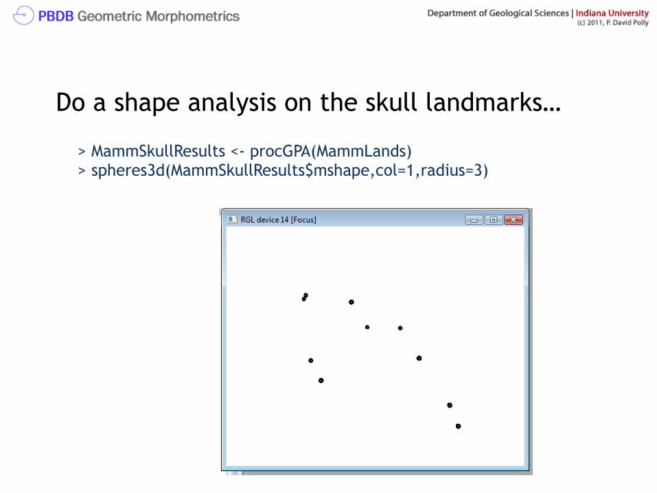
> shapepca(MammSkullResults)

Create similar vector plot with shapepca()

Consensus shape is shown with red balls, the deforma>on on each PC is shown by a colored vector

> shapepca(MammResults,scores3d=T)

PC1

PC2

PC3

Create PC plot with shapepca()

Trees a method for summarizing morphometric results

Apodemus

Marmota

Spermophilus

Any >me you have three or more OTUs* – regardless of whether they are popula>ons, stra>graphic samples, species, genera, families, or whatever – they will be linked by a phylogene>c tree that may introduce autocorrela>on between the more closely related taxa.

In palaeontology, nearly all morphological data have a phylogenetic component

* OTU – Operational Taxonomic Unit, shorthand for “group in question”

Controversies about phylogenetic ‘signal’ in morphometric data

•  Some people, usually cladists, argue that morphometric data do not have phylogenetic signal because they measure ‘overall’ similarity.

•  Others argue that morphometric data do not have phylogenetic signal because they are mostly ‘adaptive’.

•  And yet others argue that morphometric data do not have phylogenetic signal because they are mostly ‘non-genetic’.

•  And a few argue that morphometric data do not have phylogenetic signal because they are merely morphological, not molecular....

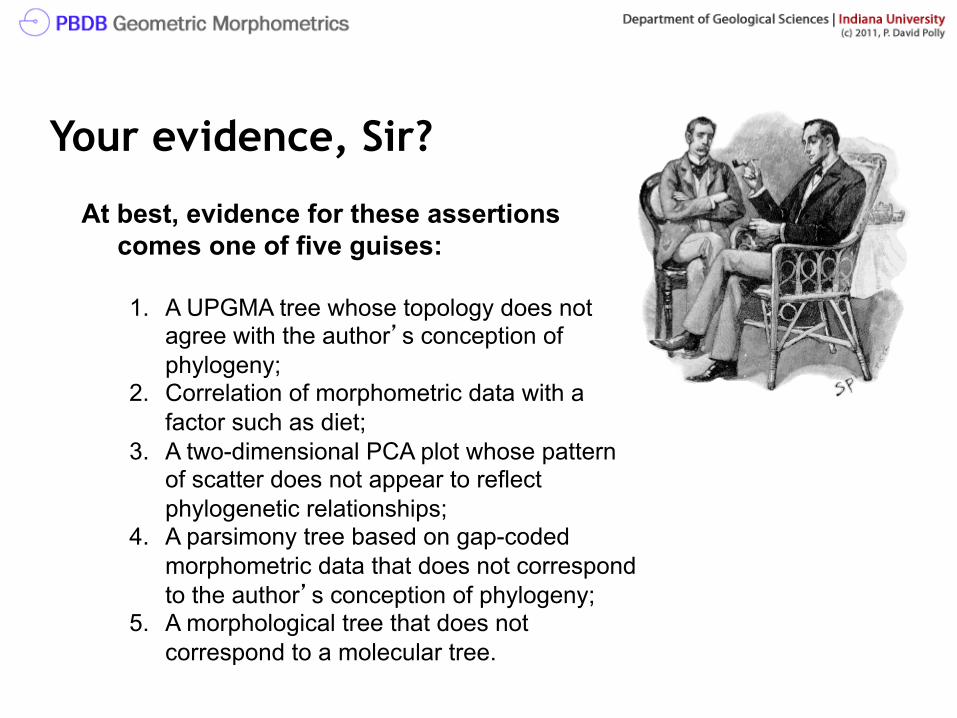
Your evidence, Sir?

At best, evidence for these assertions comes one of five guises:

1.  A UPGMA tree whose topology does not

agree with the author’s conception of phylogeny;

2.  Correlation of morphometric data with a factor such as diet;

3.  A two-dimensional PCA plot whose pattern of scatter does not appear to reflect phylogenetic relationships;

4.  A parsimony tree based on gap-coded morphometric data that does not correspond to the author’s conception of phylogeny;

5.  A morphological tree that does not correspond to a molecular tree.

Alternative hypotheses

If morphometric variation isn’t ‘phylogenetic’ what is it?

1.  Non-genetic, entirely environmentally plastic response to local conditions met by an organism during its lifetime.

2.  Non-existent.

3.  Measurement error.

4.  Evidence for special creation.

All but the last have strong evidence to the contrary.

(This slide is sarcasm, by the way)

Approaches to the question that are more sophisticated than “your data are not phylogenetic”/”yes they are!”

•  How much of morphometric variation can be explained by phylogenetic history?

•  Under what circumstances phylogenetic history be recovered from morphometric data?

•  With what accuracy can phylogenetic history be recovered from morphometric data?

•  When does phylogenetic history interfere with recovering other relationships?

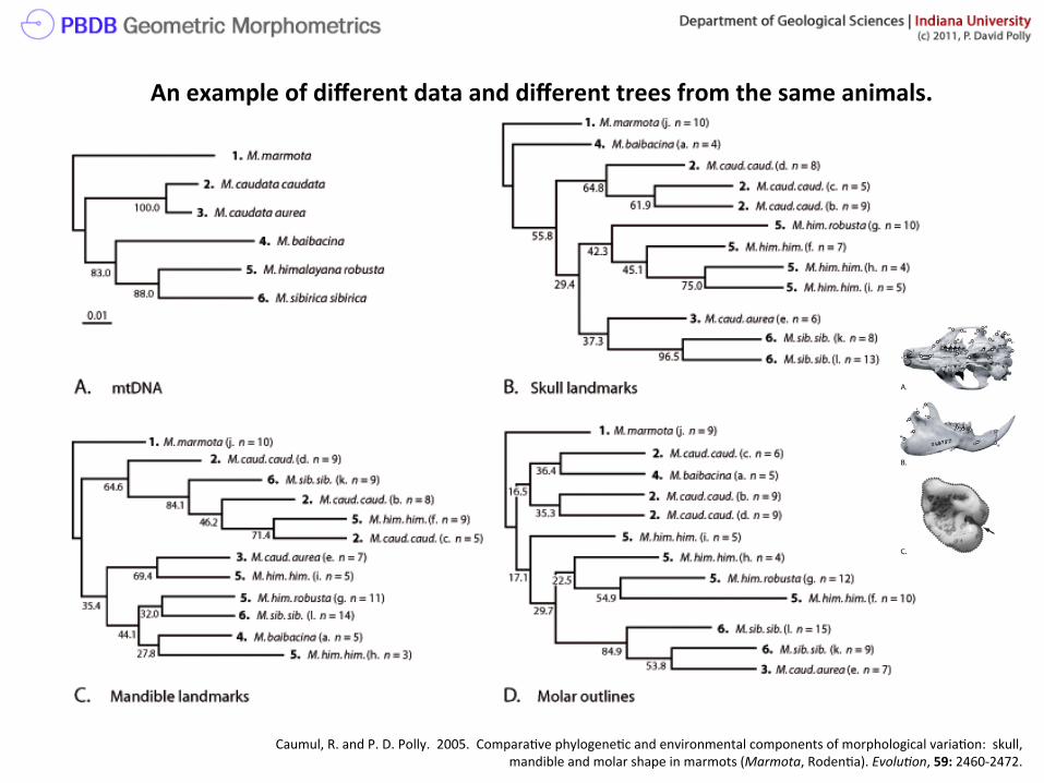
Caumul, R. and P. D. Polly. 2005. Compara>ve phylogene>c and environmental components of morphological varia>on: skull, mandible and molar shape in marmots (Marmota, Roden>a). Evolu5on, 59: 2460-‐2472.

An example of different data and different trees from the same animals.

Path Analysis (a controlled regression)

% not explained by the various factors


“good” trees

Take home message: phylogene>c ‘signal’ doesn’t have to be huge to get a phylogene>cally meaningful tree, but such trees don’t come from every data set


What do we know about quantitative variation in morphological form (size and shape)? As with so many things, the answer depends on what par5cular morphological structure or varia5on is being discussed. (Here I’ll comment on vertebrate skeletons).

1.   Morphometric variation is largely, but not entirely heritable. Typical heritability studies put the value at 40%-70% heritable (percentage of variation that is passed from parent to offspring), high for traits that are measured by geneticists.

2.   Morphometric traits evolve quickly. Compared to the gain and loss of structures (i.e., cladistic state changes of the ideal type), the size and shape of structures changes rapidly. (Something that ought to be obvious based on logic alone).

3.   Size and shape of homologous structures are often constrained by common ‘homologous’ functions. Once a structure has arisen, it often maintains a similar function throughout phylogenetic history (though there are notable exceptions). Thus the size and shape of that structure have functional constraints imposed on them. And morphometric comparisons are normally limited to structures that are found in all the OTUs being studied.

Some hierarchical considerations....

Varia?on within popula?ons is largely free of phylogene>c effects and so is an appropriate system for measuring rela>onship of shape to factors such as body size, la>tude, etc.

Varia?on among species (or other OTUs) is normally influenced both by phylogene>c history and adap>ve selec>on. The two may be difficult to disentangle (indeed, the two are themselves related). Among species in a appropriate system to measure disparity, adap>ve similarity, etc.

Phylogenetic correlations....

When doing statistics of shape data to other variables (e.g., regression or MANOVA), one must be careful of phylogenetic correlations when the data consist of different species or populations, some of which are more closely related and some of which are more distantly related.

Phylogeny makes such data non-independent because similarity in shape and the other variable may be due to common ancestry rather than direct causal association.

Methods for removing phylogene>c correla>on and for mapping morphometric varia>on onto a tree

Phylogene?c independent contrasts. A simple method for removing effects of shared history from data. Invented by Joe Felsenstein. Elaborated by Andy Purvis.

Phylogene?c General Linear Models (PGLM) A more sophis>cated method for assessing phylogene>c correla>on and for mapping traits onto a tree. Developed by Mar>ns and Hansen (1997).

Squared Change Parsimony A cladist-‐friendly name for what is virtually the same things as the maximum-‐likelihood model of doing PGLM. Developed by Maddison (1991).

Felsenstein, J. 1985. Phylogenies and the compara>ve method. The American Naturalist 125: 1-‐15.

Maddison, W. P. 1991. Squared-‐change parsimony reconstruc>ons of ancestral states for con>nuous-‐valued characters on a phylogene>c tree. Systema>c Zoology, 40: 304-‐314.

Mar>ns, E. P. and T. F. Hansen. 1997. Phylogenies and the compara>ve method: a general approach to incorpora>ng phylogene>c informa>on into the analysis of interspecific data. American Naturalist, 149: 646-‐667.

Remember, however….. Many important func?onal or environmental proper?es have arisen by EVOLUTION •  Morphology that has evolved with a specific func>on results from phylogene>c

processes •  Removing the effects of phylogeny will remove all such rela>onships from your

data •  For example, removing the effects of phylogeny from morphometric data will

remove the effects of

•  Adapta>ons to new climates or environments •  Adapta>ons to new diets or locomo>on •  Key innova>ons or adap>ve radia>on

Phylogene>c approach to study of adapta>on does not remove the effects of phylogeny

Greene, HW. 1986. Diet and arboreality in the Emerald monitor, Varanus prasinus, with comments on the study of adapta>on. Fieldiana Zoology, 31: 1-‐12.

Summary: phylogeny and morphometrics 1.  Morphometric data which include more than one species always have a

phylogene>c component to shape varia>on 2.  Phylogeny can some>mes be recovered from morphometric data in op>mal

circumstances: a.  rate of evolu>on is compa>ble with phylogene>c depth (i.e., fast enough to

have differences but not too fast to have lots of homoplasy) b.  When gene>c/developmental underpinnings of the morphology are

heritable and have mul>ple sources 3.  Morphometric data are a weak tool for phylogeny reconstruc>on because:

a.  limita>on that landmarks must be placed on homologous points, which excludes apomorphies

b.  quan>ta>ve traits usually evolve quicker than gain and loss of meristric structures

c.  func>onal and developmental-‐gene>c constraints on homologous structure usually promote homoplasy

Why not build a tree? (Pros)

•  Summarizes similarities and differences in shape across the whole shape in a single, intuitive diagram.

•  For biological data drawn from more than one species, the null assumption is that shape differences should be distributed in a tree-like hierarchy because of phylogeny.

•  Morphometric trees can easily be compared to other trees (e.g., molecular phylogenies) using standard methods.

•  Looks impressive.

Why build a tree? (cons)

•  Your data might be the sort that does not have a natural hierarchical distribution.

•  A tree necessarily distorts shape relations in order to force multivariate relationships into a single diagram.

•  Trees forcefully represented complicated relationships and don’t necessarily encourage thoughtful exploration of data.

•  Assessing statistical support for trees based on morphometric shape is complicated and in its infancy.

•  Morphometric trees are bad, ‘phenetics’!

Terminology OTU (Operational Taxonomic Unit). This is a generic way of referring to whatever the things are on your tree (specimens, species means, handaxes, whatever).

Tree. A branching diagram that connects objects by their similarity. Many criteria can be used for constructing a tree. In all cases, an assumption in building a tree is that object differences are structured such that they form a hierarchically nested pattern.

Algorithm. The programming steps used to calculate the tree.

Cladistic parsimony. A method for constructing trees for purposes of phylogeny reconstruction that requires traits to be categorized into ‘primitive’ and ‘derived’, hence an algorithm that cannot be applied to continuous quantitative data such as geometric shape.

Quantitative or continuous data. Data that are ‘measured’ and which can have a state equal to any real number. Geometric shape is an example of quantitative data.

Meristic or discrete data. Data in which a trait can have only a specific ‘state’, often coded using integers. Often this is the presence or absence of things like digits.

More Terminology

More Terminology Phenetics. Tree building based on quantitative data. The term is normally used in a derogatory sense for comparison to cladistic parsimony because quantitative tree building methods do not formally divide variables into primitive and derived states.

Pairwise distance. Quantitative ‘distance’ between two OTUs. In geometric morphometrics the pairwise distance is most logically the Procrustes distance, which is the same as a Euclidean distance. There are many kinds of ‘distances’ that can be calculated, however.

Patristic distance. The distance between two OTUs along the branches of the tree. This is usually different than the true pairwise distance because of compromises made in constructing the tree.

Exact algorithm. A tree building algorithm that follows a single train of steps to calculate a tree.

Optimizing algorithm. A tree building algorithm that finds the ‘best’ tree using a certain criterion. A more-or-less exhaustive search is made through all possible trees to find the one that best fits the criterion.

Statistical method. An optimizing algorithm that incorporates a probability model based on variances and statistical distributions. Maximum likelihood is such a method.

Maximum likelihood. A general statistical method for estimating parameters like regression lines. In this discussion it refers to a specific statistically-based tree algorithm.

Even More Terminology

Three types of Trees Additive. The length of branches on the tree correspond to change along the branch (i.e., to the shape distance between points on the tree). Neighbor-joining trees are an example of an additive tree.

Ultrametric tree. A tree constructed so that the branch lengths all end at the same distance from the root of the tree. This is a plausible requirement because many OTUs are taxa and have evolved from a common ancestor, all to the present day. However, the ‘true’ distance between OTUs may have to be distorted more to construct such a tree than with an additive tree. The ‘cluster analysis’ algorithm of PAST produces such trees.

Unnamed type of tree. One whose branches simply show the clustering relations of the OTUs, but don’t also show a ‘patristic distance’.

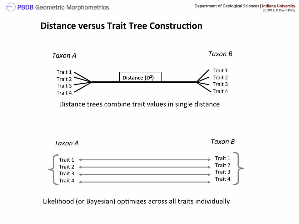
And two other ways of thinking about trees Distance matrix trees. For these trees, a pairwise distance matrix is first constructed. The algorithm fits the tree using those distances. A distance matrix is very closely related to a covariance matrix, but doesn’t keep track of individual traits (which is important to diagnose what supports different branches). Both the cluster and neighbor-joining methods in PAST are distance methods.

Trait based trees. A tree constructed from individual traits. Maximum likelihood is such a method. In theory, the value of each trait can be determined for each node. For geometric shape, this means that a shape can be constructed anywhere on the tree.

Taxon A

Trait 1 Trait 2 Trait 3 Trait 4

Taxon B


Distance (D2)

Taxon A


Taxon B


Likelihood (or Bayesian) op>mizes across all traits individually

Distance trees combine trait values in single distance

Distance versus Trait Tree Construc?on

Types of Distance Trees UPGMA: an ultrametric tree that can be calculated using any of the same distances, as well as with different joining methods.

Neighbour joining: an additive tree that can be calculated using several distances.

Types of Distances

Euclidean distance. For shape data, the Euclidean distance is equivalent to Procrustes distance and is recommended.

Some distances will produce errors because they are based on Gene Frequencies and cannot be calculated from data containing negative values or values greater than 1.0.

Assumptions of distance matrix algorithms 1. Each distance is measured independently from the others: no item of data contributes to more than one distance. (normally not true because any individual OTU is compared to all of the other OTUs to build the distance matrix) 2. The distance between each pair of taxa is drawn from a distribution with an expectation which is the sum of values (in effect amounts of evolution) along the tree from one tip to the other. The variance of the distribution is proportional to a power p of the expectation. (means effectively that no unusual directional selection or unequal rates of evolution have occurred). (from Felsenstein’s PHYLIP documentation)

Making distance trees in R Calculate distance matrix:

> myDists <- dist(results$rawscores)

Cluster the data:

> myClusters <- hclust(myDists)

(with option method=“average” you get a UPGMA tree, with method=“complete” you get a complete linkage tree)

Plot the tree:

> plot(myClusters)

1 3

2

4 5

4050

6070

80

Cluster Dendrogram

hclust (*, "complete")dist(results$rawscores)

Hei

ght

Maximum likelihood trees (Trait-based trees) Optimizes the tree statistically, keeping all the traits separate rather than combining them into a single distance.

The algorithm finds the tree topology that maximizes the likelihood of the shape data in your sample having evolved given that tree and a Brownian motion model of evolution (i.e., no long-term directional selection and no strong stabilizing selection).

The algorithm combines the probabilities associated with each OTU to find a branching pattern that connects them, presuming that the probability distribution of each is centered on its own value and that the variance of the distribution is a portion of the variance among all the OTUs.

To create a ML tree in PHYLIP 1.  Save scores in a space delimited text file, ensure that OTU names are

10 characters long (no more, and fill out short names with spaces), place the number of OTUs and the number of traits in the first line by themselves.

2.  Save the file with the name ‘infile’ in the PHYLIP folder.

3.  Start CONTML module by double-clicking it. (Continuous Maximum likelihood).

4.  Choose options: ‘C” for continuous traits, “J’ jumble trees (add any odd number).

5.  Click ‘Y’ to start the program.

6.  View results in ‘outfile’, which is a text file showing tree and statistics, and in ‘treefile’, which is a file that can be viewed and edited in TreeView.

PHYLIP is at hsp://evolu>on.gene>cs.washington.edu/phylip.html

Identifying groups in large sample: Kernel Density Estimate Clustering

Baylac, Villemant, and Simbolotti. 2003. Combining geometric morphometrics with pattern recognition for the investigation of species complexes. Biological Journal of the Linnean Society, 80: 89-98.

Software: R statistical and mathematical language.

1. Install package KernSmooth.

2. Load package KernSmooth

> library(KernSmooth)

3. Recreate results for the mandibles of the three rodent species

4. Perform a Kernal Density Es>mate on the scores from the first two PC axes:

> est <-‐ bkde2D(results$rawscores[,1:2],bandwidth=c(0.01,.01))

> contour(est$x1,est$x2,est$uat)

> persp(est$uat)

NB: bandwidth values need to be smaller than the range of scores on PC1 and PC2, but not too much smaller. Experiment to see what happens with smaller and larger bandwidths.

Perform a Kernel Density Estimate to find groups

Reconstruc?ng ancestral shape: how to do geometric genealogy

Sorex

Blarina

Apodemus

Marmota

Spermophilus

1

2

3

4

5

6

7

8

9

> plot.phylo(mytree) > >plabels() > nodelabels()

Newick format tree: ((Sorex:1,Blarina:1):2 ,((Spermophilus:1,Marmota:1):1,Apodemus:2):1);

library(ape)

tree <-‐ read.nexus(‘filename’) -‐-‐ reads a NEXUS phylogene>c tree file tree <-‐ read.tree(‘filename’) -‐-‐ reads a Newick or New Hampshire tree file plot.phylo(tree) – plots the tree on the screen ace(data, tree) – es>mates ancestral states on tree for a univariate trait data

Necessary ingredients for modeling shape on a phylogene?c tree

Hurdles to overcome in modeling ancestral shapes

1.  Order of taxa on tree is mostly likely different from their order in the shape dataset. The order must be the same.

Solu5on: create a variable taxonorder. For each taxon on the tree, enter the posi>on of that taxon in the original data set. For example if tree taxon 1 was the third taxon in the original data, then the first number in taxonorder should be 3. > taxonorder <-‐ c(1,3,4,2,5) > results$rawscores[taxonorder,1]

2.  ace() fails when the data are PC scores. Probably this is due to the fact that the mean of the scores is exactly 0.0, which creates division by zero somewhere in the algorithm.

Solu5on: add an arbitrary number to the scores, calculated the ancestral states, and then subtract that number back out. > ace(results$rawscores[taxonorder,1]+100, mytree)$ace -‐ 100

Calculate the ancestral values of the PC scores

> PC1ancestors <-‐ ace(results$rawscores[taxonorder,1]+100,mytree)$ace-‐100 > PC2ancestors <-‐ ace(results$rawscores[taxonorder,2]+100,mytree)$ace-‐100 > PC3ancestors <-‐ ace(results$rawscores[taxonorder,3]+100,mytree)$ace-‐100 Model the landmarks for each of the posi>ons in shape space > ancestorNode6 <-‐ PC1ancestors[1] * results$pcar[,1]+PC2ancestors[1] * results$pcar[,2]+PC3ancestors[1] * results$pcar[,3]+results$mshape > tpsgrid(results$mshape,ancestorNode6)

-200 0 200

-200

0200

Sorex

Blarina

Apodemus

Marmota

Spermophilus

Plot the ancestral shapes on your tree

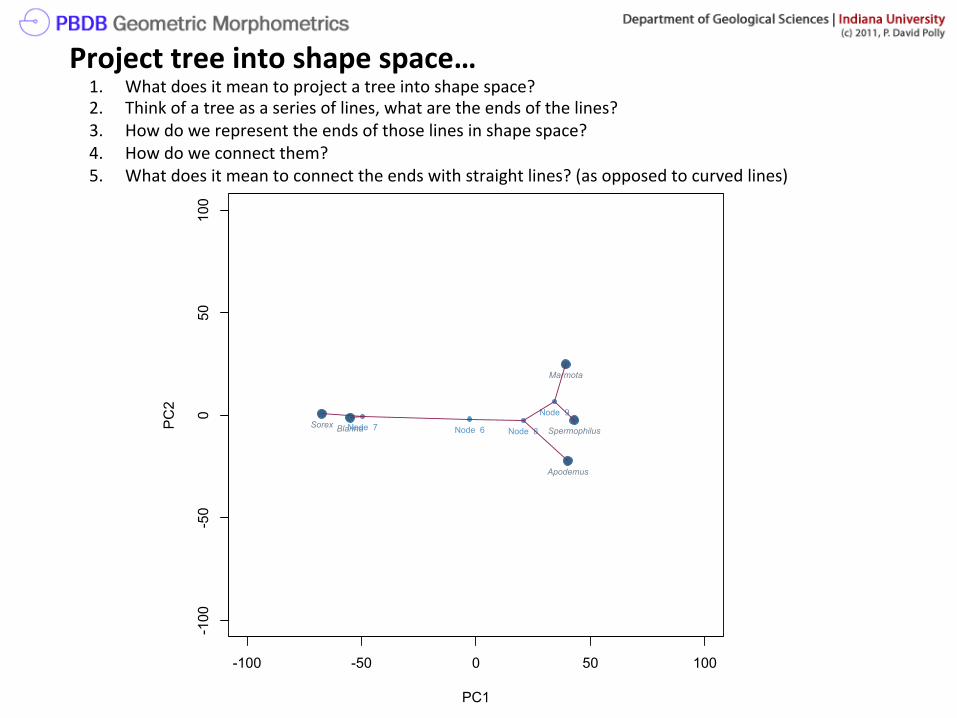
Project tree into shape space… 1.  What does it mean to project a tree into shape space? 2.  Think of a tree as a series of lines, what are the ends of the lines? 3.  How do we represent the ends of those lines in shape space? 4.  How do we connect them? 5.  What does it mean to connect the ends with straight lines? (as opposed to curved lines)

-100 -50 0 50 100

-100

-50

050

100

PC1

PC2

Sorex

Marmota

Blarina

Apodemus

SpermophilusNode 6Node 7 Node 8

Node 9

To project a tree into shape space…

> plot(c(-‐100,100),c(-‐100,100),xlab="PC1",ylab="PC2",type="n") > points(results$rawscores,col='Steelblue4',cex=2.0,pch=20) > text(results$rawscores,genuslabels,pos=1,cex=.6,col="slategrey",font=3) > points(PC1ancestors,PC2ancestors,col='Steelblue3',cex=1.0,pch=20) > text(PC1ancestors,PC2ancestors,paste("Node ",6:9),col='Steelblue3',cex=.6,pos=1) What does this create? > treeendpoints <-‐ rbind(results$rawscores[taxonorder,1:2],cbind(PC1ancestors,PC2ancestors)) What are these and how can we use them? > mytree$edge Why does the following line work? > lines(treeendpoints[mytree$edge[1,],]) The following line plots all the lines in the shrew and marmot tree: > for(i in 1:8) lines(treeendpoints[mytree$edge[i,],],cex=1.2,col="violetred4")

3D Data, Phylogenetics, and Treesg562/PBDB2013/Day 5A - Phylogeny and trees.pdf... evidence for...

Documents

Transcript of 3D Data, Phylogenetics, and Treesg562/PBDB2013/Day 5A - Phylogeny and trees.pdf... evidence for...