3D · PDF file · 2014-09-28We begin with a problem whose solution will be reused...

© 2014 Steve Marschner • Cornell CS4620 Fall 2014 • Lecture 12

3D Viewing

CS 4620 Lecture 12

1


Viewing, backward and forward

• So far have used the backward approach to viewing– start from pixel– ask what part of scene projects to pixel– explicitly construct the ray corresponding to the pixel

• Next will look at the forward approach– start from a point in 3D– compute its projection into the image

• Central tool is matrix transformations– combines seamlessly with coordinate transformations used to position

camera and model– ultimate goal: single matrix operation to map any 3D point to its correct

screen location.

2


Forward viewing

• Would like to just invert the ray generation process

• Problem 1: ray generation produces rays, not points in scene

• Inverting the ray tracing process requires division for the perspective case

3


Mathematics of projection

• Always work in eye coords– assume eye point at 0 and plane perpendicular to z

• Orthographic case– a simple projection: just toss out z

• Perspective case: scale diminishes with z– and increases with d

4


Pipeline of transformations

• Standard sequence of transforms

5

✐

✐

✐

✐

✐

✐

✐

✐

7.1. Viewing Transformations 147

object space

world space

camera space

canonicalview volume

scre

en

sp

ace

modelingtransformation

viewporttransformation

projectiontransformation

cameratransformation

Figure 7.2. The sequence of spaces and transformations that gets objects from their

original coordinates into screen space.

space) to camera coordinates or places them in camera space. The projection

transformation moves points from camera space to the canonical view volume.

Finally, the viewport transformation maps the canonical view volume to screen Other names: camera

space is also “eye space”

and the camera

transformation is

sometimes the “viewing

transformation;” the

canonical view volume is

also “clip space” or

“normalized device

coordinates;” screen space

is also “pixel coordinates.”

space.

Each of these transformations is individually quite simple. We’ll discuss them

in detail for the orthographic case beginning with the viewport transformation,

then cover the changes required to support perspective projection.

7.1.1 The Viewport Transformation

We begin with a problemwhose solution will be reused for any viewing condition.

We assume that the geometry we want to view is in the canonical view volume The word “canonical” crops

up again—it means

something arbitrarily

chosen for convenience.

For instance, the unit circle

could be called the

“canonical circle.”

and we wish to view it with an orthographic camera looking in the −z direction.The canonical view volume is the cube containing all 3D points whose Cartesian

coordinates are between −1 and +1—that is, (x, y, z) ∈ [−1, 1]3 (Figure 7.3).We project x = −1 to the left side of the screen, x = +1 to the right side of thescreen, y = −1 to the bottom of the screen, and y = +1 to the top of the screen.

Recall the conventions for pixel coordinates fromChapter 3: each pixel “owns”

a unit square centered at integer coordinates; the image boundaries have a half-

unit overshoot from the pixel centers; and the smallest pixel center coordinates


Parallel projection: orthographic

to implement orthographic, just toss out z:

6


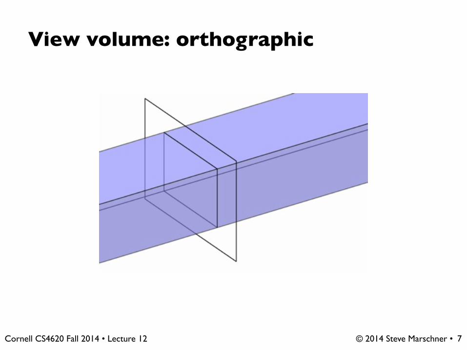
View volume: orthographic

7


Viewing a cube of size 2

• Start by looking at a restricted case: the canonical view volume

• It is the cube [–1,1]3, viewed from the z direction

• Matrix to project it into a square image in [–1,1]2 is trivial:

8

�

⇤1 0 0 00 1 0 00 0 0 1

⇥

⌅


Viewing a cube of size 2

• To draw in image, need coordinates in pixel units, though

• Exactly the opposite of mapping (i,j) to (u,v) in ray generation

9

–1–1

1

1 –.5–.5

ny – .5

nx – .5


Windowing transforms

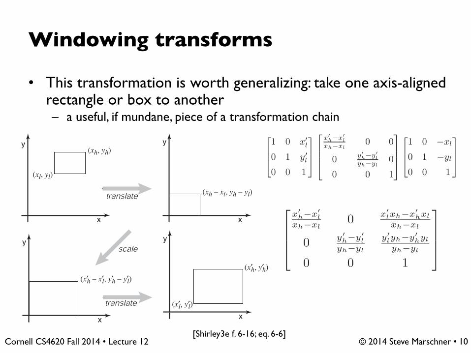
• This transformation is worth generalizing: take one axis-aligned rectangle or box to another– a useful, if mundane, piece of a transformation chain

[Shirley3e f. 6-16; eq. 6-6] 10

✐

✐

✐

✐

✐

✐

✐

✐

6.3. Translation 135

In 3D, the same technique works: we can add a fourth coordinate, a homoge-

neous coordinate, and then we have translations:

⎡

⎢

⎢

⎣

1 0 0 xt

0 1 0 yt

0 0 1 zt

0 0 0 1

⎤

⎥

⎥

⎦

⎡

⎢

⎢

⎣

xyz1

⎤

⎥

⎥

⎦

=

⎡

⎢

⎢

⎣

x + xt

y + yt

z + zt

1

⎤

⎥

⎥

⎦

.

Again, for a vector, the fourth coordinate is zero and the vector is thus unaffected

by translations.

Example 8 (Windowing Transformations) Often in graphics we need to create

a transform matrix that takes points in the rectangle [xl, xh] × [yl, yh] to therectangle [x′

l, x′h] × [y′

l, y′h]. This can be accomplished with a single scale and

translate in sequence. However, it is more intuitive to create the transform from a

sequence of three operations (Figure 6.16):

1. Move the point (xl, yl) to the origin.

2. Scale the rectangle to be the same size as the target rectangle.

3. Move the origin to point (x′l, y

′l).

(xl, yl)

(x′l, y′l)

(xh, yh)

(x′h, y′h)

(xh – xl, yh – yl)

(x′h – x′l, y′h – y′l)

Figure 6.16. To take one rectangle (window) to the other, we first shift the lower-left cornerto the origin, then scale it to the new size, and then move the origin to the lower-left cornerof the target rectangle.

✐

✐

✐

✐

✐

✐

✐

✐

136 6. Transformation Matrices

Remembering that the right-hand matrix is applied first, we can write

window = translate (x′l, y

′l) scale

(

x′h − x′

l

xh − xl,y′

h − y′l

yh − yl

)

translate (−xl,−yl)

=

⎡

⎢

⎣

1 0 x′l

0 1 y′l

0 0 1

⎤

⎥

⎦

⎡

⎢

⎢

⎣

x′

h−x′

l

xh−xl0 0

0 y′

h−y′

l

yh−yl0

0 0 1

⎤

⎥

⎥

⎦

⎡

⎢

⎣

1 0 −xl

0 1 −yl

0 0 1

⎤

⎥

⎦

=

⎡

⎢

⎢

⎣

x′

h−x′

l

xh−xl0 x′

lxh−x′

hxl

xh−xl

0 y′

h−y′

l

yh−yl

y′

lyh−y′

hyl

yh−yl

0 0 1

⎤

⎥

⎥

⎦

.

(6.6)

It is perhaps not surprising to some readers that the resulting matrix has the form

it does, but the constructive process with the three matrices leaves no doubt as to

the correctness of the result.

An exactly analogous construction can be used to define a 3D windowing

transformation, which maps the box [xl, xh]×[yl, yh]×[zl, zh] to the box [x′l, x

′h]×

[y′l, y

′h] × [z′l, z

′h]

⎡

⎢

⎢

⎢

⎢

⎢

⎣

x′

h−x′

l

xh−xl0 0 x′

lxh−x′

hxl

xh−xl

0 y′

h−y′

l

yh−yl0 y′

lyh−y′

hyl

yh−yl

0 0 z′

h−z′

l

zh−zl

z′

lzh−z′

hzl

zh−zl

0 0 0 1

⎤

⎥

⎥

⎥

⎥

⎥

⎦

. (6.7)

It is interesting to note that if we multiply an arbitrary matrix composed of

scales, shears and rotations with a simple translation (translation comes second),

we get⎡

⎢

⎢

⎣

1 0 0 xt

0 1 0 yt

0 0 1 zt

0 0 0 1

⎤

⎥

⎥

⎦

⎡

⎢

⎢

⎣

a11 a12 a13 0a21 a22 a23 0a31 a32 a33 00 0 0 1

⎤

⎥

⎥

⎦

=

⎡

⎢

⎢

⎣

a11 a12 a13 xt

a21 a22 a23 yt

a31 a32 a33 zt

0 0 0 1

⎤

⎥

⎥

⎦

.

Thus we can look at any matrix and think of it as a scaling/rotation part and a

translation part because the components are nicely separated from each other.

An important class of transforms are rigid-body transforms. These are com-

posed only of translations and rotations, so they have no stretching or shrinking

of the objects. Such transforms will have a pure rotation for the aij above.

✐

✐

✐

✐

✐

✐

✐

✐




′l) scale

(

x′h − x′

l

xh − xl,y′

h − y′l

yh − yl

)


=

⎡

⎢

⎣

1 0 x′l

0 1 y′l

0 0 1

⎤

⎥

⎦

⎡

⎢

⎢

⎣

x′

h−x′

l

xh−xl0 0

0 y′

h−y′

l

yh−yl0

0 0 1

⎤

⎥

⎥

⎦

⎡

⎢

⎣

1 0 −xl

0 1 −yl

0 0 1

⎤

⎥

⎦

=

⎡

⎢

⎢

⎣

x′

h−x′

l

xh−xl0 x′

lxh−x′

hxl

xh−xl

0 y′

h−y′

l

yh−yl

y′

lyh−y′

hyl

yh−yl

0 0 1

⎤

⎥

⎥

⎦

.

(6.6)






′h]×

[y′l, y

′h] × [z′l, z

′h]

⎡

⎢

⎢

⎢

⎢

⎢

⎣

x′

h−x′

l

xh−xl0 0 x′

lxh−x′

hxl

xh−xl

0 y′

h−y′

l

yh−yl0 y′

lyh−y′

hyl

yh−yl

0 0 z′

h−z′

l

zh−zl

z′

lzh−z′

hzl

zh−zl

0 0 0 1

⎤

⎥

⎥

⎥

⎥

⎥

⎦

. (6.7)



we get⎡

⎢

⎢

⎣

1 0 0 xt

0 1 0 yt

0 0 1 zt

0 0 0 1

⎤

⎥

⎥

⎦

⎡

⎢

⎢

⎣

a11 a12 a13 0a21 a22 a23 0a31 a32 a33 00 0 0 1

⎤

⎥

⎥

⎦

=

⎡

⎢

⎢

⎣

a11 a12 a13 xt

a21 a22 a23 yt

a31 a32 a33 zt

0 0 0 1

⎤

⎥

⎥

⎦

.






�

⇤xscreen

yscreen

1

⇥

⌅ =

�

⇤nx2 0 nx�1

2

0 ny

2ny�1

2

0 0 1

⇥

⌅

�

⇤xcanonical

ycanonical

1

⇥

⌅


Viewport transformation

11

–1–1

1

1 –.5–.5

ny – .5

nx – .5


Viewport transformation

• In 3D, carry along z for the ride– one extra row and column

12

Mvp =

�

⇧⇧⇤

nx2 0 0 nx�1

2

0 ny

2 0 ny�12

0 0 1 00 0 0 1

⇥

⌃⌃⌅


Orthographic projection

• First generalization: different view rectangle– retain the minus-z view direction

– specify view by left, right, top, bottom (as in RT)– also near, far

13

✐

✐

✐

✐

✐

✐

✐

✐


Figure 7.5. The orthographic view volume is along the negative z-axis, so f is a morenegative number than n, thus n > f.

the bounding planes as follows:

x = l ≡ left plane,

x = r ≡ right plane,

y = b ≡ bottom plane,

y = t ≡ top plane,

z = n ≡ near plane,

z = f ≡ far plane.

That vocabulary assumes a viewer who is looking along the minus z-axis with

Figure 7.4. The ortho-graphic view volume.

his head pointing in the y-direction. 1 This implies that n > f , which may beunintuitive, but if you assume the entire orthographic view volume has negative zvalues then the z = n “near” plane is closer to the viewer if and only if n > f ;here f is a smaller number than n, i.e., a negative number of larger absolute valuethan n.

This concept is shown in Figure 7.5. The transform from orthographic view

volume to the canonical view volume is another windowing transform, so we can

simply substitute the bounds of the orthographic and canonical view volumes into

Equation 6.7 to obtain the matrix for this transformation: n and f appear in whatmight seem like reverseorder because n − f ,rather than f − n, is apositive number.

Morth =

⎡

⎢

⎢

⎣

2r−l 0 0 − r+l

r−l

0 2

t−b0 − t+b

t−b

0 0 2n−f

− n+tn−f

0 0 0 1

⎤

⎥

⎥

⎦

(7.3)

1Most programmers find it intuitive to have the x-axis pointing right and the y-axis pointing up. Ina right-handed coordinate system, this implies that we are looking in the −z direction. Some systemsuse a left-handed coordinate system for viewing so that the gaze direction is along +z. Which is bestis a matter of taste, and this text assumes a right-handed coordinate system. A reference that argues

for the left-handed system instead is given in the notes at the end of the chapter.


Clipping planes

• In object-order systems we always use at least twoclipping planes that further constrain the view volume– near plane: parallel to view plane; things between it and the

viewpoint will not be rendered– far plane: also parallel; things behind it will not be rendered

• These planes are:– partly to remove unnecessary stuff (e.g. behind the camera)– but really to constrain the range of depths

(we’ll see why later)

14


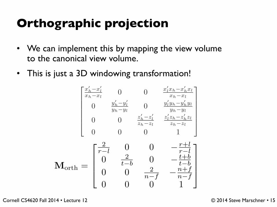
Orthographic projection

• We can implement this by mapping the view volumeto the canonical view volume.

• This is just a 3D windowing transformation!

15

✐

✐

✐

✐

✐

✐

✐

✐




′l) scale

(

x′h − x′

l

xh − xl,y′

h − y′l

yh − yl

)


=

⎡

⎢

⎣

1 0 x′l

0 1 y′l

0 0 1

⎤

⎥

⎦

⎡

⎢

⎢

⎣

x′

h−x′

l

xh−xl0 0

0 y′

h−y′

l

yh−yl0

0 0 1

⎤

⎥

⎥

⎦

⎡

⎢

⎣

1 0 −xl

0 1 −yl

0 0 1

⎤

⎥

⎦

=

⎡

⎢

⎢

⎣

x′

h−x′

l

xh−xl0 x′

lxh−x′

hxl

xh−xl

0 y′

h−y′

l

yh−yl

y′

lyh−y′

hyl

yh−yl

0 0 1

⎤

⎥

⎥

⎦

.

(6.6)






′h]×

[y′l, y

′h] × [z′l, z

′h]

⎡

⎢

⎢

⎢

⎢

⎢

⎣

x′

h−x′

l

xh−xl0 0 x′

lxh−x′

hxl

xh−xl

0 y′

h−y′

l

yh−yl0 y′

lyh−y′

hyl

yh−yl

0 0 z′

h−z′

l

zh−zl

z′

lzh−z′

hzl

zh−zl

0 0 0 1

⎤

⎥

⎥

⎥

⎥

⎥

⎦

. (6.7)



we get⎡

⎢

⎢

⎣

1 0 0 xt

0 1 0 yt

0 0 1 zt

0 0 0 1

⎤

⎥

⎥

⎦

⎡

⎢

⎢

⎣

a11 a12 a13 0a21 a22 a23 0a31 a32 a33 00 0 0 1

⎤

⎥

⎥

⎦

=

⎡

⎢

⎢

⎣

a11 a12 a13 xt

a21 a22 a23 yt

a31 a32 a33 zt

0 0 0 1

⎤

⎥

⎥

⎦

.






Morth =

�

⇧⇧⇤

2r�l 0 0 � r+l

r�l

0 2t�b 0 � t+b

t�b

0 0 2n�f �n+f

n�f

0 0 0 1

⇥

⌃⌃⌅


Camera and modeling matrices

• We worked out all the preceding transforms starting from eye coordinates– before we do any of this stuff we need to transform into that space

• Transform from world (canonical) to eye space is traditionally called the viewing matrix– it is the canonical-to-frame matrix for the camera frame

– that is, Fc–1

• Remember that geometry would originally have been in the object’s local coordinates; transform into world coordinates is called the modeling matrix, Mm

• Note many programs combine the two into a modelview matrix and just skip world coordinates

16


Viewing transformation

the camera matrix rewrites all coordinates in eye space

17


Orthographic transformation chain

• Start with coordinates in object’s local coordinates• Transform into world coords (modeling transform, Mm)

• Transform into eye coords (camera xf., Mcam = Fc–1)

• Orthographic projection, Morth

• Viewport transform, Mvp

18

⇤

⌥⌥⇧

xs

ys

zc

1

⌅

��⌃ =

⇤

⌥⌥⇧

nx2 0 0 nx�1

2

0 ny

2 0 ny�12

0 0 1 00 0 0 1

⌅

��⌃

⇤

⌥⌥⇧

2r�l 0 0 � r+l

r�l

0 2t�b 0 � t+b

t�b

0 0 2n�f �n+f

n�f

0 0 0 1

⌅

��⌃

�u v w e0 0 0 1

⇥�1

Mm

⇤

⌥⌥⇧

xo

yo

zo

1

⌅

��⌃

ps = MvpMorthMcamMmpo


Perspective projection

similar triangles:

20


Homogeneous coordinates revisited

• Perspective requires division– that is not part of affine transformations– in affine, parallel lines stay parallel

• therefore not vanishing point• therefore no rays converging on viewpoint

• “True” purpose of homogeneous coords: projection

21


Homogeneous coordinates revisited

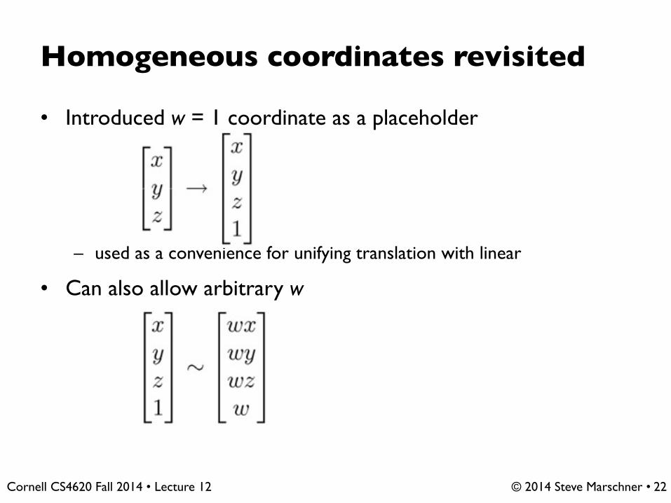
• Introduced w = 1 coordinate as a placeholder

– used as a convenience for unifying translation with linear

• Can also allow arbitrary w

22


Implications of w

• All scalar multiples of a 4-vector are equivalent

• When w is not zero, can divide by w– therefore these points represent “normal” affine points

• When w is zero, it’s a point at infinity, a.k.a. a direction– this is the point where parallel lines intersect– can also think of it as the vanishing point

• Digression on projective space

23


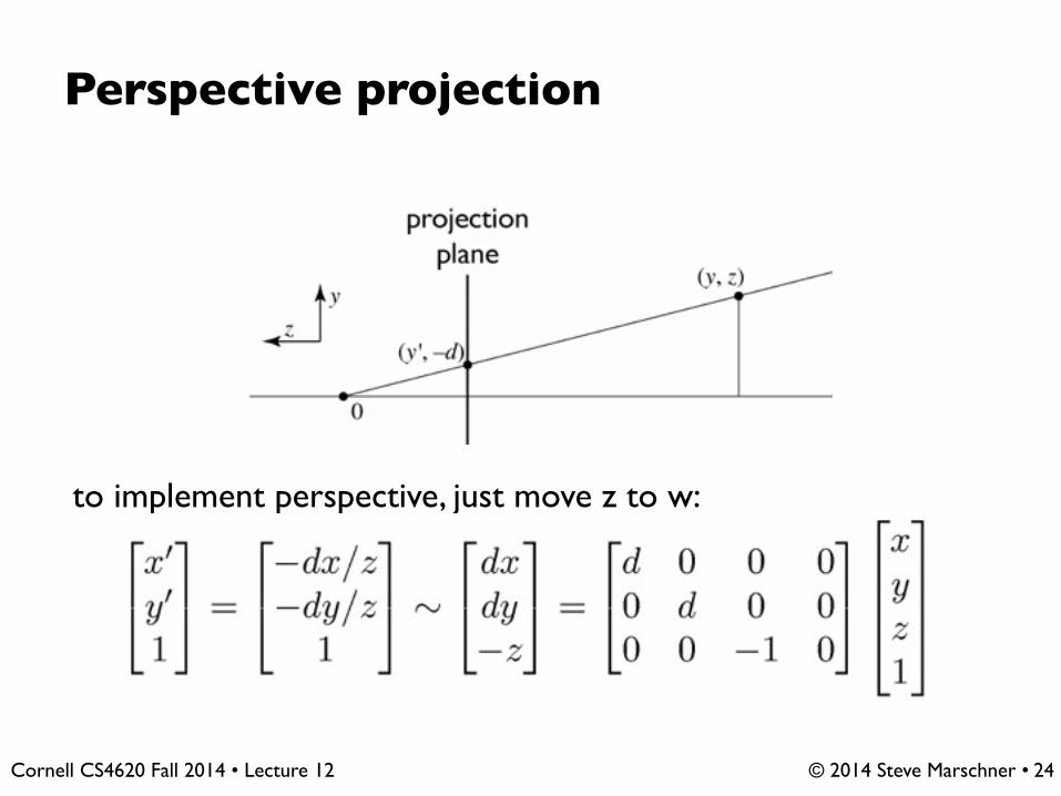
Perspective projection

to implement perspective, just move z to w:

24


View volume: perspective

25


View volume: perspective (clipped)

26


Carrying depth through perspective

• Perspective has a varying denominator—can’t preserve depth!

• Compromise: preserve depth on near and far planes

– that is, choose a and b so that z’(n) = n and z’(f) = f.

27


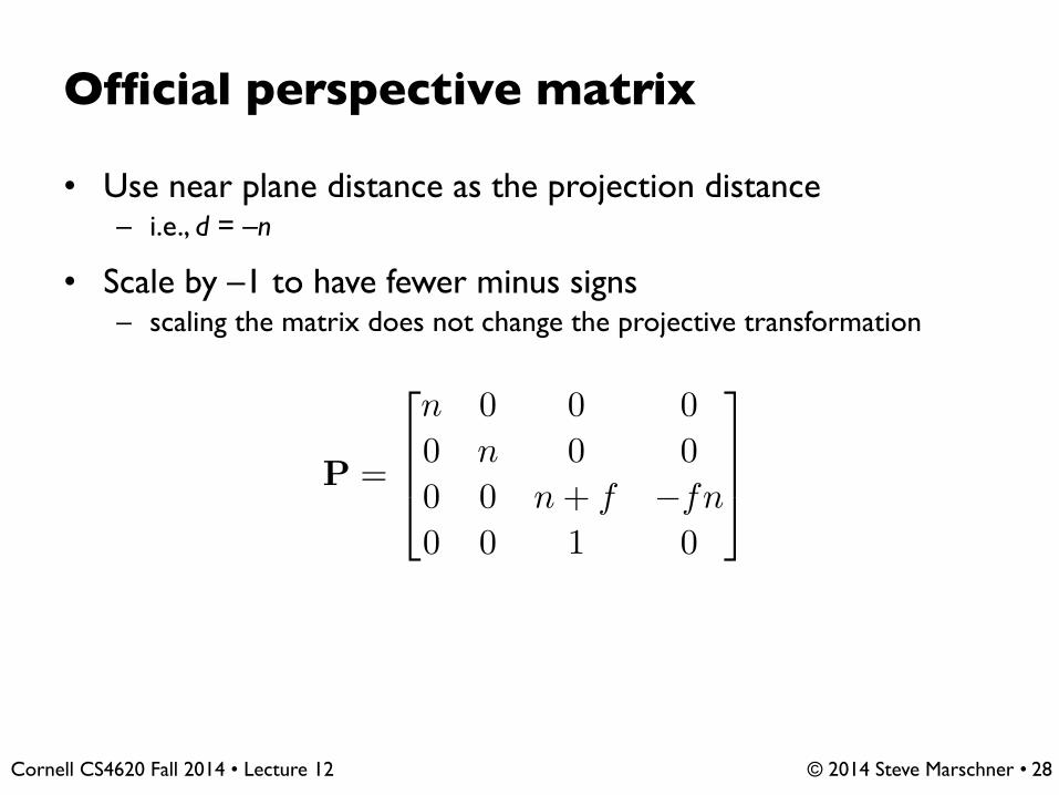
Official perspective matrix

• Use near plane distance as the projection distance– i.e., d = –n

• Scale by –1 to have fewer minus signs– scaling the matrix does not change the projective transformation

28

P =

�

⇧⇧⇤

n 0 0 00 n 0 00 0 n + f �fn0 0 1 0

⇥

⌃⌃⌅


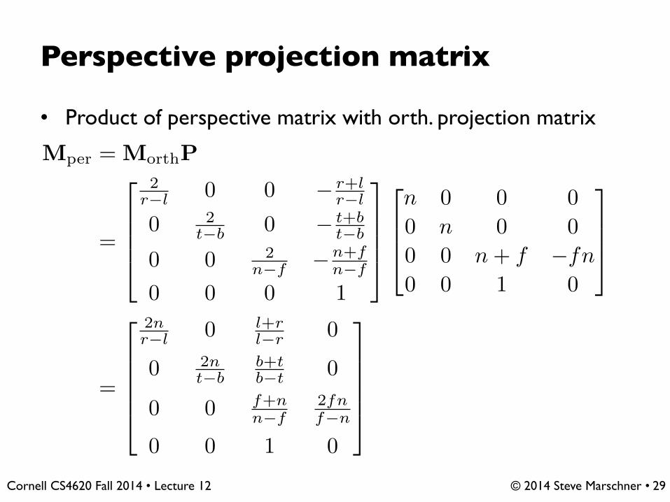
Perspective projection matrix

• Product of perspective matrix with orth. projection matrix

29

Mper = MorthP

=

�

⇧⇧⇧⇤

2r�l 0 0 � r+l

r�l

0 2t�b 0 � t+b

t�b

0 0 2n�f �n+f

n�f

0 0 0 1

⇥

⌃⌃⌃⌅

�

⇧⇧⇤

n 0 0 00 n 0 00 0 n + f �fn0 0 1 0

⇥

⌃⌃⌅

=

�

⇧⇧⇧⇧⇤

2nr�l 0 l+r

l�r 0

0 2nt�b

b+tb�t 0

0 0 f+nn�f

2fnf�n

0 0 1 0

⇥

⌃⌃⌃⌃⌅


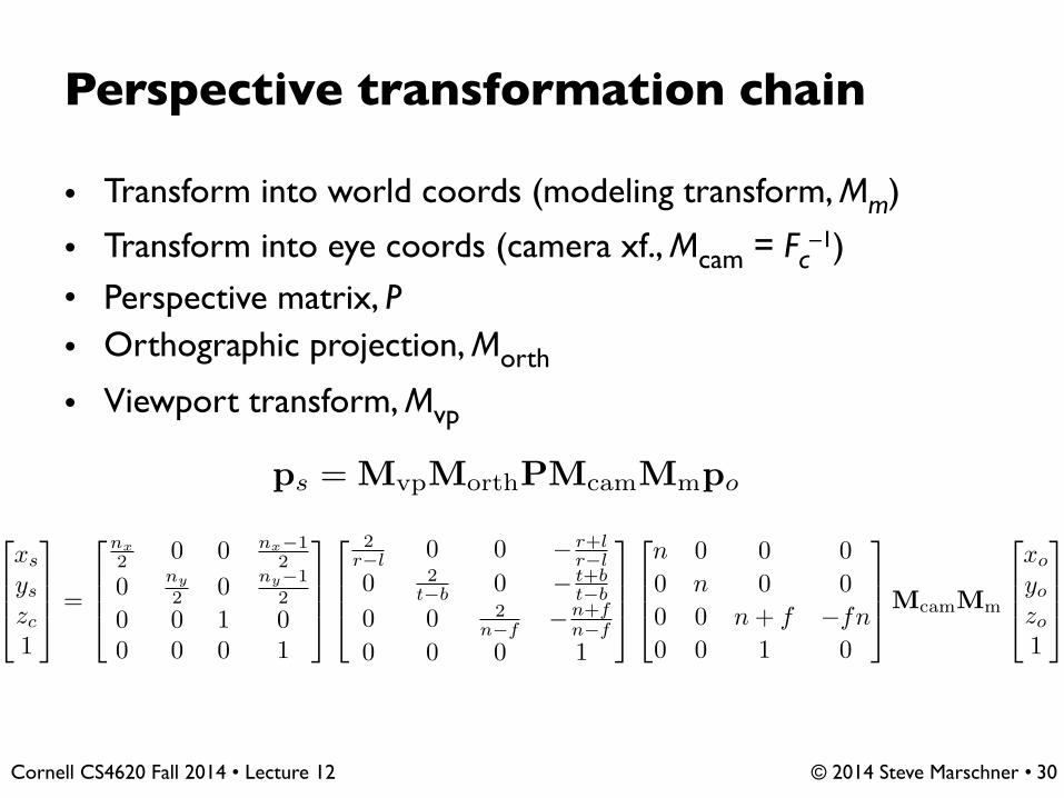
Perspective transformation chain

• Transform into world coords (modeling transform, Mm)

• Transform into eye coords (camera xf., Mcam = Fc–1)

• Perspective matrix, P• Orthographic projection, Morth

• Viewport transform, Mvp

30

ps = MvpMorthPMcamMmpo

�

⇧⇧⇤

xs

ys

zc

1

⇥

⌃⌃⌅ =

�

⇧⇧⇤

nx2 0 0 nx�1

2

0 ny

2 0 ny�12

0 0 1 00 0 0 1

⇥

⌃⌃⌅

�

⇧⇧⇤

2r�l 0 0 � r+l

r�l

0 2t�b 0 � t+b

t�b

0 0 2n�f �n+f

n�f

0 0 0 1

⇥

⌃⌃⌅

�

⇧⇧⇤

n 0 0 00 n 0 00 0 n + f �fn0 0 1 0

⇥

⌃⌃⌅McamMm

�

⇧⇧⇤

xo

yo

zo

1

⇥

⌃⌃⌅


Pipeline of transformations

• Standard sequence of transforms

31

✐

✐

✐

✐

✐

✐

✐

✐


object space

world space

camera space

canonicalview volume

scre

en

sp

ace

modelingtransformation

viewporttransformation

projectiontransformation

cameratransformation

Figure 7.2. The sequence of spaces and transformations that gets objects from their

original coordinates into screen space.

space) to camera coordinates or places them in camera space. The projection

transformation moves points from camera space to the canonical view volume.

Finally, the viewport transformation maps the canonical view volume to screen Other names: camera

space is also “eye space”

and the camera

transformation is

sometimes the “viewing

transformation;” the

canonical view volume is

also “clip space” or

“normalized device

coordinates;” screen space

is also “pixel coordinates.”

space.

Each of these transformations is individually quite simple. We’ll discuss them

in detail for the orthographic case beginning with the viewport transformation,

then cover the changes required to support perspective projection.

7.1.1 The Viewport Transformation

We begin with a problemwhose solution will be reused for any viewing condition.

We assume that the geometry we want to view is in the canonical view volume The word “canonical” crops

up again—it means

something arbitrarily

chosen for convenience.

For instance, the unit circle

could be called the

“canonical circle.”

and we wish to view it with an orthographic camera looking in the −z direction.The canonical view volume is the cube containing all 3D points whose Cartesian

coordinates are between −1 and +1—that is, (x, y, z) ∈ [−1, 1]3 (Figure 7.3).We project x = −1 to the left side of the screen, x = +1 to the right side of thescreen, y = −1 to the bottom of the screen, and y = +1 to the top of the screen.

Recall the conventions for pixel coordinates fromChapter 3: each pixel “owns”

a unit square centered at integer coordinates; the image boundaries have a half-

unit overshoot from the pixel centers; and the smallest pixel center coordinates

3D · PDF file · 2014-09-28We begin with a problem whose solution will be reused...

Documents

Transcript of 3D · PDF file · 2014-09-28We begin with a problem whose solution will be reused...