382 Lecture 24
11
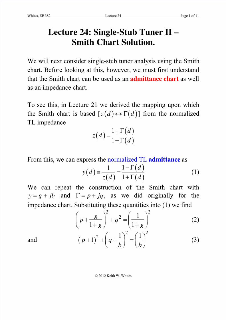
Whites, EE 382 Lecture 24 Page 1 of 11 © 2012 Keith W. Whites Lecture 24: Single-Stub Tuner II – Smith Chart Solution. We will next consider single-stub tuner analysis using the Smith chart. Before looking at this, however, we must first understand that the Smith chart can be used as an admittance chart as well as an impedance chart. To see this, in Lecture 21 we derived the mapping upon which the Smith chart is based [ z d d ] from the normalized TL impedance 1 1 d z d d From this, we can express the normalized TL admittance as 1 1 1 d y d z d d (1) We can repeat the construction of the Smith chart with y g jb and p jq , as we did originally for the impedance chart. Substituting these quantities into (1) we find 2 2 2 1 1 1 g p q g g (2) and 2 2 2 1 1 1 p q b b (3)
Transcript of 382 Lecture 24
8/13/2019 382 Lecture 24
http://slidepdf.com/reader/full/382-lecture-24 1/11
Whites, EE 382 Lecture 24 Page 1 of 11
© 2012 Keith W. Whites
Lecture 24: Single-Stub Tuner II –
Smith Chart Solution.
We will next consider single-stub tuner analysis using the Smith
chart. Before looking at this, however, we must first understand
that the Smith chart can be used as an admittance chart as well
as an impedance chart.
To see this, in Lecture 21 we derived the mapping upon which
the Smith chart is based [ z d d ] from the normalizedTL impedance
1
1
d z d
d
From this, we can express the normalized TL admittance as
111
d y d z d d
(1)
We can repeat the construction of the Smith chart with
y g jb and p jq , as we did originally for the
impedance chart. Substituting these quantities into (1) we find2 2
2 1
1 1
g p q
g g
(2)
and 2 2
2 1 11 p q
b b
(3)

8/13/2019 382 Lecture 24
http://slidepdf.com/reader/full/382-lecture-24 2/11
Whites, EE 382 Lecture 24 Page 2 of 11
A Smith admittance chart can be constructed based on these two
equations for circles in the p-q plane:
Re p d
d q Im
8/13/2019 382 Lecture 24
http://slidepdf.com/reader/full/382-lecture-24 3/11
Whites, EE 382 Lecture 24 Page 3 of 11
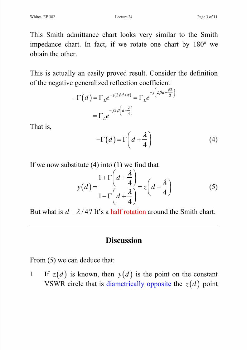
This Smith admittance chart looks very similar to the Smith
impedance chart. In fact, if we rotate one chart by 180º we
obtain the other.
This is actually an easily proved result. Consider the definition
of the negative generalized reflection coefficient
2
2 2
24
j d j d
L L
j d
L
d e e
e
That is,
4
d d
(4)
If we now substitute (4) into (1) we find that
1
44
14
d
y d z d
d
(5)
But what is / 4d ? It’s a half rotation around the Smith chart.
Discussion
From (5) we can deduce that:
1. If z d is known, then y d is the point on the constant
VSWR circle that is diametrically opposite the z d point

8/13/2019 382 Lecture 24
http://slidepdf.com/reader/full/382-lecture-24 4/11
Whites, EE 382 Lecture 24 Page 4 of 11
on the Smith chart. (In this context, remember that a QWT
is an impedance inverter device.)
2.
The Smith chart can be used either as an impedance chart or as an admittance chart. Rather than keeping these two
types of charts around, we can use one for either impedance
or admittance calculations. The following example should
help you understand this.
3. One subtlety with these mixed Smith charts is that
generalized reflection coefficients are only correctlyrepresented on impedance charts when plotting
normalized impedances and on admittance charts when
plotting normalized admittances. You’ll read negative
generalized reflection coefficients otherwise (for
admittances on impedance charts and impedances on
admittance charts).
Example N24.1: Use the Smith chart to compute the normalized
input admittance of the TL shown below.

8/13/2019 382 Lecture 24
http://slidepdf.com/reader/full/382-lecture-24 5/11
Whites, EE 382 Lecture 24 Page 5 of 11
0
50 500 1 1
50
L Z j z j
Z
p.u.
10 0.5 0.50
y j z
p.u.S
Rotating 0.362 “towards generator ,” we can read from the
Smith chart:
1.7 1.1 z L j and 0.42 0.28 y L j
[Exact: 1.682 1.103 z L j and 0.4157 0.2727 y L j .]

8/13/2019 382 Lecture 24
http://slidepdf.com/reader/full/382-lecture-24 6/11
Whites, EE 382 Lecture 24 Page 6 of 11

8/13/2019 382 Lecture 24
http://slidepdf.com/reader/full/382-lecture-24 7/11
Whites, EE 382 Lecture 24 Page 7 of 11
Single-Stub Matching with the Smith Chart
As we saw in the previous lecture, the single-stub tuner
geometry attached to a TL is
Recall that the operation of the single-stub tuner requires that
1. A length sd is chosen such that 1 y has a real part = 1.2. The imaginary part of 1 y is negated by the stub
susceptance after choosing the proper lengths
L .
We can perform these steps using only the Smith chart as our
calculator . This process will be illustrated by an example.
Example N24.2: Using the Smith chart, design a shorted single-
stub tuner to match the load 35 47.5 L Z j to a TL with
characteristic resistance 0 50 Z .

8/13/2019 382 Lecture 24
http://slidepdf.com/reader/full/382-lecture-24 8/11
Whites, EE 382 Lecture 24 Page 8 of 11
The normalized load impedance and admittance are:
0.70 0.95 L z j p.u. and 0.50 0.68
L y j p.u.S
Steps:
1. Locate 0.50 0.68 L
y j p.u.S on the Smith
admittance chart.
2. Draw the constant VSWR circle using a compass.
3. Draw the line segment from the origin to L y [this is
the vector 0 / 4 ]. Rotate this vector towardsthe source until it intersects the unit conductance
circle. Along this circle Re 1 y d .
This is really the intersection of the constant VSWR
circle for this load with the unit conductance circle.
There will be two solutions. Both of these give
1 11 y jb .
For this example, we find from the Smith chart that
(I) 11 1.2 y j
(II) 11 1.2 y j
4. From these rotations we can determines
d as
(I) 0.168 0.109 0.059sd
(II) 0.332 0.109 0.223sd
8/13/2019 382 Lecture 24
http://slidepdf.com/reader/full/382-lecture-24 9/11
Whites, EE 382 Lecture 24 Page 9 of 11
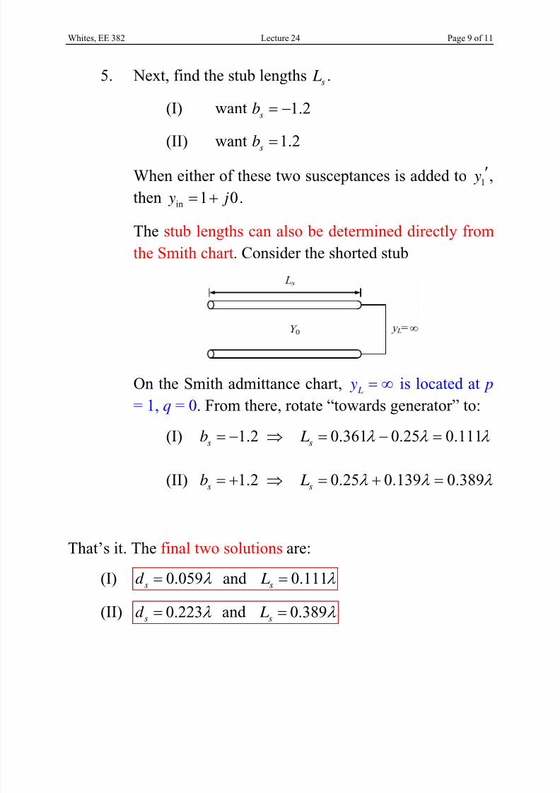
5. Next, find the stub lengthss L .
(I) want 1.2s
b
(II) want 1.2sb
When either of these two susceptances is added to1 y ,
then in 1 0 y j .
The stub lengths can also be determined directly from
the Smith chart. Consider the shorted stub
On the Smith admittance chart, L y is located at p
= 1, q = 0. From there, rotate “towards generator” to:
(I) 1.2 0.361 0.25 0.111s s
b L
(II) 1.2 0.25 0.139 0.389s s
b L
That’s it. The final two solutions are:(I) 0.059
sd and 0.111
s L
(II) 0.223sd and 0.389s
L

8/13/2019 382 Lecture 24
http://slidepdf.com/reader/full/382-lecture-24 10/11
Whites, EE 382 Lecture 24 Page 10 of 11
We will check these two solutions using the results of the
analytical analysis from the last lecture:

8/13/2019 382 Lecture 24
http://slidepdf.com/reader/full/382-lecture-24 11/11
Whites, EE 382 Lecture 24 Page 11 of 11
2
21.191
1
L
s
L
b
for 0.5116 1.367 L rad.
11 1tan 2
2 2 4
/ 4 1.904 2 1/ 4 0
/ 4 0.8299 2 1/ 4 0
L
ss
s
s
bd n
n b
n b
Then
for 1.191s
b with n = -1 (so that 0s
d ) gives 0.2235s
d ,
for 1.191s
b with n = 0 gives 0.05896s
d .
and
for 1.191sb gives
2
1 11 tan 0.38882 2
L
s
L
L
for 1.191sb gives
2
111
tan 0.11122
L
s
L
L