3.7 Isotope Effect - Homepage – Institute for Particle ... · Figure 3.45: Comparison of the...

3–45 Molecular Universe, HS 2009, D. Fluri, ETH Zurich

3.7 Isotope Effect

In this section we will study a first astrophysical application of molecular spectroscopy, namely the determination of abundance ratios of different isotopes. Molecules serve as a much more ideal tool to distinguish different isotopes than atoms. This is because the presence of more or less neutrons in the nucleus of a specific chemical element does not strongly modify the electric field and thus has only a small influence on the electron configuration. The same is true for the electron configuration of molecules of course. However, the energy of nuclear motion in molecules due to vibration and rotation is influenced already to first order if the number of neutrons and thus the mass of the nucleus is changed. Thus, isotopic molecules have different frequencies of vibrations and rotations.

First we will consider the modification of molecular spectra due to the presence of different isotopes. Then we will look at several examples that illustrate how knowledge of isotope ratios allows us to gain insight into astrophysical objects and processes. Later, in Chapter 6 (Astrobiology), we will discuss an additional important example where knowledge of isotope ratios is crucial for determining the origin of water on Earth.

3.7.1 Vibration

For isotopic molecules, i.e. molecules that differ only by the mass of one or both of the nuclei but not by their atomic number (for example 1H35Cl and 1H37Cl), the vibrational frequencies are obviously different. Assuming harmonic vibrations the (classical) vibrational frequency is given by (see Eq. (3.33))

osc

1 ,

2

kνπ µ

= (3.88)

where the force constant k, since it is determined by the electronic motion only, is exactly the same for different isotopic molecules, whereas the reduced mass µ is different. Therefore, if we let the superscript “i” distinguish an isotopic molecule from the “ordinary” molecule we have

iosc

iosc

.ν µ ρν µ

= = (3.89)

The heavier isotope has the smaller frequency. If the superscript “i” refers to the heavier isotope the constant ρ will be smaller than 1. For example, the values of ρ for the pairs 1H35Cl and 1H37Cl, 1H35Cl and 2H35Cl, 10BO and 11BO, and 16O16O and 16O18O are 0.99924, 0.71720, 0.97177, and 0.97176, respectively.

By substituting Eq. (3.89) into Eq. (3.38) we find for the vibrational levels of two isotopic molecules (still assuming harmonic oscillations)

( ) ( )i ie e

1 1= .

2 2G Gυ ω υ ρω υ ρ υ = + + =

(3.90)

3 Molecular Spectroscopy 3–46

Therefore, the separation of corresponding vibrational levels in two isotopic molecules are somewhat shifted (and as a result spectral lines are also shifted). The levels of the lighter isotope always lie higher than those of the heavier isotope.

If anharmonicity is taken into account, the calculations become rather more involved and will not be reproduced here. The formulae for the energy levels are found to be in a very good approximation

( )2 3

e e e e e

1 1 1 ,

2 2 2G x yυ ω υ ω υ ω υ = + − + + + +

… (3.91)

( )2 3

i 2 3e e e e e

1 1 1 .

2 2 2G x yυ ρω υ ρ ω υ ρ ω υ = + − + + + +

… (3.92)

In other words, the vibrational constants are modified as

ie e

i i 2e e e e

i i 3e e e e

,

,

.

x x

y y

ω ρωω ρ ωω ρ ω

=

=

=

(3.93)

3.7.2 Rotation

Since the reduced mass is inversely proportional to the rotational constant B, molecules containing heavy isotopes have rotational lines corresponding to lower quantum energies and smaller line spacing. Specifically, we find for the rotational constant B of the two isotopic molecules

2

i 2e ei 2

eq

= .2

B Br hc

ρµ

= ℏ (3.94)

Note that the internuclear distances in diatomic (and polyatomic) molecules are entirely determined by the electronic structure. They are therefore exactly equal in isotopic molecules as long as no vibration occurs. The rotational energies of the two isotopic molecules are thus connected by

i 2 2e e( 1) ( 1) .iF B J J B J J Fρ ρ= + = + = (3.95)

Rotational levels of the heavier molecule have smaller energies. Furthermore, the separation of neighboring lines in the rotational spectrum (which is 2B in first approximation) differs for isotopic molecules. For example, for the 12CO molecule, 2B is found to be 3.842 cm–1, and for the 13CO molecule containing the heavier isotope of carbon,

Figure 3.43: The isotope effect on the rota-tional energy levels and the corresponding rotational spectrum of the CO molecule. The line shifts are exaggerated in this drawing. From Haken & Wolf (2006).


2B is found to be 3.673 cm–1. Figure Figure 3.43 shows the resulting differences in the rotational spectra of CO containing the isotopes 12C and 13C.

For simultaneous vibration and rotation, in a first approximation, we simply have to add the vibrational and rotational isotope effects. As a result, the lines of a rotation-vibration band of an isotopic molecule do not have exactly the same separations as the lines of the “normal” molecule. In other words, the isotope displacement between corresponding lines of the two bands is dependent on J.

Since the rotational energies are smaller than the vibrational energies, the rotational isotope shift is, in general, smaller than the vibrational one, despite the fact that the former scales with ρ2 while the latter scales with ρ.

For more precise calculation, it is necessary to take into account the interaction of vibration and rotation, i.e. the rotational constants α, β, D, and possibly higher order ones. To a very good approximation we may use

i 4e e

i 3

i 5

,

,

.

D Dρα ρ αβ ρ β

=

==

(3.96)

3.7.3 Astrophysical Examples

Nucleosynthesis: Overview

The detection of isotopic molecules enables measurements of isotope ratios, which provide information on details of the nucleosynthesis:

• 7Li/ 6Li ⇒ lithium production rate • 12C/13C ⇒ CNO cycle efficiency and mixing processes in stellar envelopes • 16O/17O/18O ⇒ 3α-process efficiency • 24Mg/25Mg/26Mg ⇒ carbon burning efficiency • 32S/34S ⇒ oxygen burning efficiency • 56Fe/57Fe/58Fe ⇒ supernova explosion details

In the following, as an example, we will have a closer look at the astrophysical diagnostics with the 12C/13C ratio. Apart from studying nucleosynthesis at different stages of the stellar evolution, measurements of isotope ratios serve as a test of primordial nucleosynthesis and thus of cosmology. Isotope ratios also provide insight into the chemical evolution of our galaxy (see below).

Solar Isotope Ratios

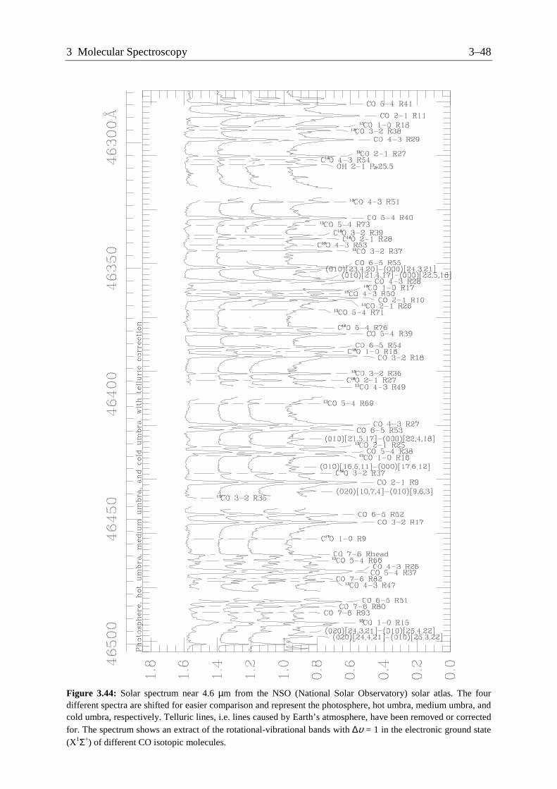
Figure 3.44 shows infrared bands with ∆υ = 1 of isotopic CO molecules in the solar spectrum. Comparison of such observations with synthetic, i.e. computed, spectra allows us to determine isotope ratios for carbon and oxygen atoms. The analysis yields solar isotope ratios 12C/13C = 80±1, 16O/17O = 1700±220, and 16O/18O = 440±6 (Ayres et al. 2006).


Figure 3.44: Solar spectrum near 4.6 µm from the NSO (National Solar Observatory) solar atlas. The four different spectra are shifted for easier comparison and represent the photosphere, hot umbra, medium umbra, and cold umbra, respectively. Telluric lines, i.e. lines caused by Earth’s atmosphere, have been removed or corrected for. The spectrum shows an extract of the rotational-vibrational bands with ∆υ = 1 in the electronic ground state (X1Σ+) of different CO isotopic molecules.


Since the solar atmosphere is not simply an optically thin gas, the calculation of the solar spectrum involves radiative transfer calculations based on solar model atmospheres. The model atmosphere provides the height stratification of the thermodynamic properties such as temperature, pressure, and density within the solar atmosphere.

Stellar 12C/13C ratios

Analogously to the Sun we can determine isotope ratios of other stars. The 12C/13C isotope ratio is interesting because it is expected to change during the evolution of a star and, as a result, also during the evolution of a galaxy.

Initially, the chemical composition of a star corresponds to the local condition of the interstellar medium (ISM) and the cloud from which it was formed. Fusion in the stellar interior modifies the chemical compositions of a star during its lifetime. In the stellar spectrum this chemical evolution is only apparent if a mixing of the surface layers takes place with the center or shells where fusion occurs. Only stars of spectral class F and later have an outer convection zone, which extends all the way to the center only for late M stars. For example, the Sun, a G2 V star, possesses an outer convection zone that extends to about 0.7 R

� (as measured from the center). Therefore, in the case of the Sun, the 12C/13C ratio at the

surface is still the same as for the young Sun despite modifications resulting from the CNO-cycle that runs at the solar center. The CNO-cycle reduces 12C, increases 13C, and increases 14N abundances, so that the 12C/13C ratio actually reduces with time. Only in some phases of the late stages of stellar evolution the outer convection zone of a star like the Sun reaches down to layers where hydrogen burning has taken place so that products of the CNO-cycle are

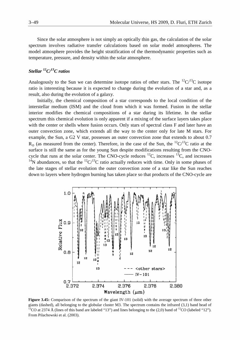
Figure 3.45: Comparison of the spectrum of the giant IV-101 (solid) with the average spectrum of three other giants (dashed), all belonging to the globular cluster M3. The spectrum contains the infrared (3,1) band head of 13CO at 2374 Å (lines of this band are labeled “13”) and lines belonging to the (2,0) band of 12CO (labeled “12”). From Pilachowski et al. (2003).

3 Molecular Spectroscopy

transported to the surface. This occurs a first time during the so called the star moves up the red giant branch in the Hertzsprungmuch lower 12C/13C ratios in the spectrum of

Figure 3.45 shows measured spectra cgiants in the globular cluster M3.IV-101 compared with three other giants is apparent even from visual inspection. The strengths of the 12CO lines, whisimilar in all four stars. Since the stars all have similar temperature, gravities, and metallicities, including oxygen and carbon abundances, the apparent weakness of the lines in IV-101 is a clear indication of a high giants in the observed cluster. The the other stars. A ratio 12C/13Cthree comparison stars (Pilachowski et al.indicates a very strong mixing. On the other hand, the other giants exhibit no Li enrichment). The higher Li abuto the presence of a Li burning shell that influences the interior temperature structure and thus the depth of the outer convection zone, apparently leading to less mixing.allow us to test and improve ste

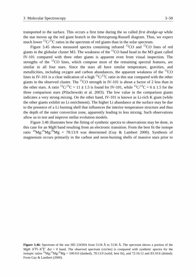
Figure 3.46 illustrates how the fitting of synthetic this case for an MgH band resulting from an electronic transition. From the best fit the isotope ratio 24Mg:25Mg:26Mg = 78:13:9 was determined (Gay & Lambert 2000). Synthesis of magnesium occurs primarily in the carb

Figure 3.46: Spectrum of the star HD 23439A from 5134 Å to 5136 Å. The spectrum shows a portion of the MgH A2Π–X2Σ+ ∆υ = 0 band. The observed spectrum (circles) is compared with synthisotopic ratios 24Mg:25Mg:26Mg = 100:0:0 (dashed), 78:13:9 (solid, best fit), and 72:16:12 and 83:10:6 (dotted). From Gay & Lambert (2000).

transported to the surface. This occurs a first time during the so called first dredgethe star moves up the red giant branch in the Hertzsprung-Russell diagram.

the spectrum of red giants than in the solar spectrumshows measured spectra containing infrared 12CO and

M3. The weakness of the 13CO band head in e other giants is apparent even from visual inspection. The

CO lines, which compose most of the remaining spectral features, are similar in all four stars. Since the stars all have similar temperature, gravities, and metallicities, including oxygen and carbon abundances, the apparent weakness of the

ear indication of a high 12C/13C ratio in this star compared with the other cluster. The 13CO strength in IV-101 is about a factor of 2 less than in

C = 11 ± 1.5 is found for IV-101, while 12C/13

(Pilachowski et al. 2003). The low value in the comparison giants indicates a very strong mixing. On the other hand, IV-101 is known as Li-the other giants exhibit no Li enrichment). The higher Li abundance at the surface may be due to the presence of a Li burning shell that influences the interior temperature structure and thus the depth of the outer convection zone, apparently leading to less mixing.allow us to test and improve stellar evolution models.

illustrates how the fitting of synthetic spectra to observations may be done, in this case for an MgH band resulting from an electronic transition. From the best fit the isotope

Mg = 78:13:9 was determined (Gay & Lambert 2000). Synthesis of magnesium occurs primarily in the carbon and neon-burning shells of massive stars prior to

Spectrum of the star HD 23439A from 5134 Å to 5136 Å. The spectrum shows a portion of the = 0 band. The observed spectrum (circles) is compared with synth

Mg = 100:0:0 (dashed), 78:13:9 (solid, best fit), and 72:16:12 and 83:10:6 (dotted).

3–50

first dredge-up while Russell diagram. Thus, we expect

solar spectrum. CO and 13CO lines of red

CO band head in the M3 giant called e other giants is apparent even from visual inspection. The

ch compose most of the remaining spectral features, are similar in all four stars. Since the stars all have similar temperature, gravities, and metallicities, including oxygen and carbon abundances, the apparent weakness of the 13CO

C ratio in this star compared with the other 101 is about a factor of 2 less than in

13C = 6 ± 1.5 for the the comparison giants

-rich K giant (while ndance at the surface may be due

to the presence of a Li burning shell that influences the interior temperature structure and thus the depth of the outer convection zone, apparently leading to less mixing. Such observations

spectra to observations may be done, in this case for an MgH band resulting from an electronic transition. From the best fit the isotope

Mg = 78:13:9 was determined (Gay & Lambert 2000). Synthesis of burning shells of massive stars prior to

Spectrum of the star HD 23439A from 5134 Å to 5136 Å. The spectrum shows a portion of the = 0 band. The observed spectrum (circles) is compared with synthetic spectra for the

Mg = 100:0:0 (dashed), 78:13:9 (solid, best fit), and 72:16:12 and 83:10:6 (dotted).


their deaths as type II supernovae. Therefore, measurements of the magnesium isotope ratio in stars provide information about the evolution of AGB stars, i.e. stars in the asymptotic giant branch.

Galactic Chemical Evolution

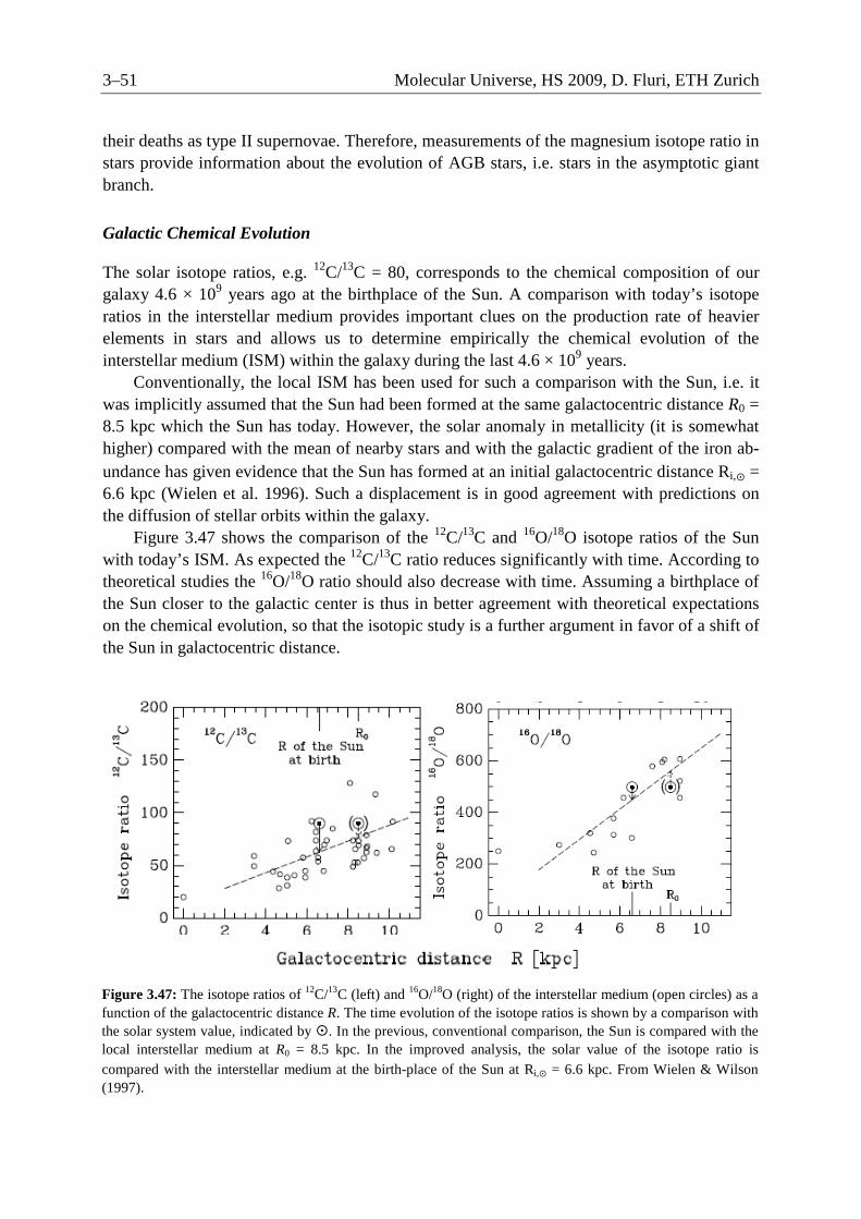
The solar isotope ratios, e.g. 12C/13C = 80, corresponds to the chemical composition of our galaxy 4.6 × 109 years ago at the birthplace of the Sun. A comparison with today’s isotope ratios in the interstellar medium provides important clues on the production rate of heavier elements in stars and allows us to determine empirically the chemical evolution of the interstellar medium (ISM) within the galaxy during the last 4.6 × 109 years.

Conventionally, the local ISM has been used for such a comparison with the Sun, i.e. it was implicitly assumed that the Sun had been formed at the same galactocentric distance R0 = 8.5 kpc which the Sun has today. However, the solar anomaly in metallicity (it is somewhat higher) compared with the mean of nearby stars and with the galactic gradient of the iron ab-undance has given evidence that the Sun has formed at an initial galactocentric distance Ri,� = 6.6 kpc (Wielen et al. 1996). Such a displacement is in good agreement with predictions on the diffusion of stellar orbits within the galaxy.

Figure 3.47 shows the comparison of the 12C/13C and 16O/18O isotope ratios of the Sun with today’s ISM. As expected the 12C/13C ratio reduces significantly with time. According to theoretical studies the 16O/18O ratio should also decrease with time. Assuming a birthplace of the Sun closer to the galactic center is thus in better agreement with theoretical expectations on the chemical evolution, so that the isotopic study is a further argument in favor of a shift of the Sun in galactocentric distance.

Figure 3.47: The isotope ratios of 12C/13C (left) and 16O/18O (right) of the interstellar medium (open circles) as a function of the galactocentric distance R. The time evolution of the isotope ratios is shown by a comparison with the solar system value, indicated by �. In the previous, conventional comparison, the Sun is compared with the local interstellar medium at R0 = 8.5 kpc. In the improved analysis, the solar value of the isotope ratio is compared with the interstellar medium at the birth-place of the Sun at Ri,� = 6.6 kpc. From Wielen & Wilson (1997).


3.8 Observation of Molecular Spectra

This section is devoted to a brief introduction into infrared and radio astronomy, including important current and future observatories and satellite missions. As we have learned pre-viously, the infrared to radio spectral regions allow us to observe rotational and rotational-vibrational spectra of molecules. In addition, the same spectral domains cover continuum spectra due to thermal and non-thermal processes. We will leave near-UV and optical obser-vations aside here as they apply also to the detection of atomic spectra and are better known.

3.8.1 Atmospheric Transmission

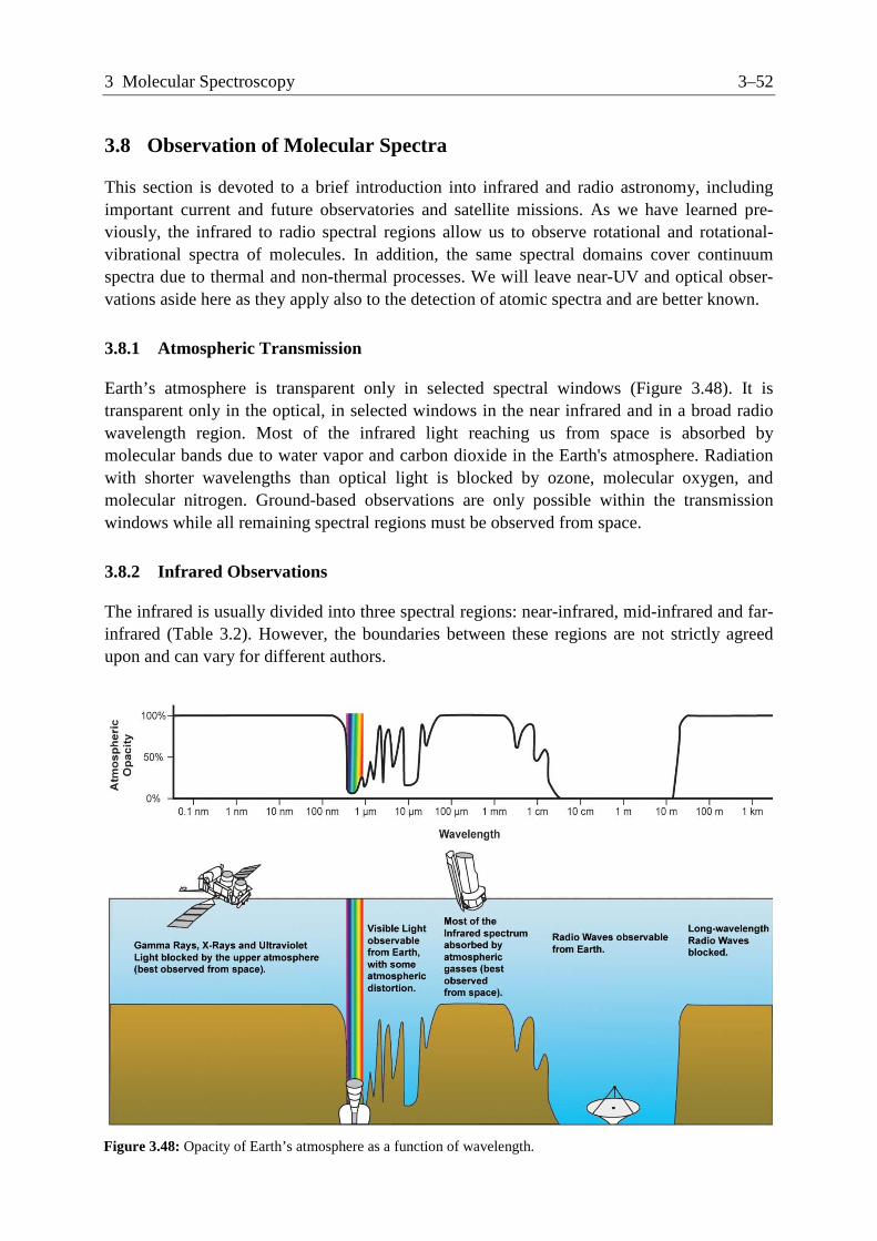
Earth’s atmosphere is transparent only in selected spectral windows (Figure 3.48). It is transparent only in the optical, in selected windows in the near infrared and in a broad radio wavelength region. Most of the infrared light reaching us from space is absorbed by molecular bands due to water vapor and carbon dioxide in the Earth's atmosphere. Radiation with shorter wavelengths than optical light is blocked by ozone, molecular oxygen, and molecular nitrogen. Ground-based observations are only possible within the transmission windows while all remaining spectral regions must be observed from space.

3.8.2 Infrared Observations

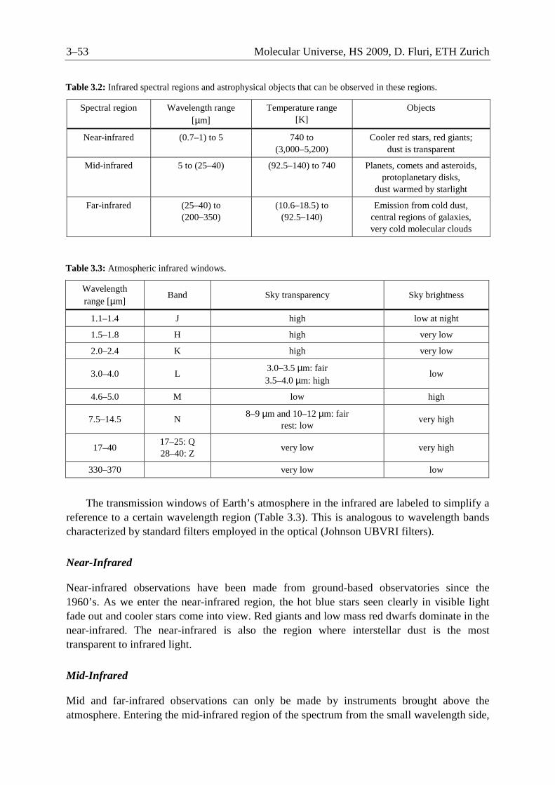
The infrared is usually divided into three spectral regions: near-infrared, mid-infrared and far-infrared (Table 3.2). However, the boundaries between these regions are not strictly agreed upon and can vary for different authors.

Figure 3.48: Opacity of Earth’s atmosphere as a function of wavelength.


The transmission windows of Earth’s atmosphere in the infrared are labeled to simplify a reference to a certain wavelength region (Table 3.3). This is analogous to wavelength bands characterized by standard filters employed in the optical (Johnson UBVRI filters).

Near-Infrared

Near-infrared observations have been made from ground-based observatories since the 1960’s. As we enter the near-infrared region, the hot blue stars seen clearly in visible light fade out and cooler stars come into view. Red giants and low mass red dwarfs dominate in the near-infrared. The near-infrared is also the region where interstellar dust is the most transparent to infrared light.

Mid-Infrared

Mid and far-infrared observations can only be made by instruments brought above the atmosphere. Entering the mid-infrared region of the spectrum from the small wavelength side,

Table 3.2: Infrared spectral regions and astrophysical objects that can be observed in these regions.

Spectral region Wavelength range [µm]

Temperature range [K]

Objects

Near-infrared (0.7–1) to 5 740 to (3,000–5,200)

Cooler red stars, red giants; dust is transparent

Mid-infrared 5 to (25–40) (92.5–140) to 740 Planets, comets and asteroids, protoplanetary disks,

dust warmed by starlight

Far-infrared (25–40) to (200–350)

(10.6–18.5) to (92.5–140)

Emission from cold dust, central regions of galaxies, very cold molecular clouds

Table 3.3: Atmospheric infrared windows.

Wavelength range [µm]

Band Sky transparency Sky brightness

1.1–1.4 J high low at night

1.5–1.8 H high very low

2.0–2.4 K high very low

3.0–4.0 L 3.0–3.5 µm: fair 3.5–4.0 µm: high

low

4.6–5.0 M low high

7.5–14.5 N 8–9 µm and 10–12 µm: fair

rest: low very high

17–40 17–25: Q 28–40: Z

very low very high

330–370 very low low


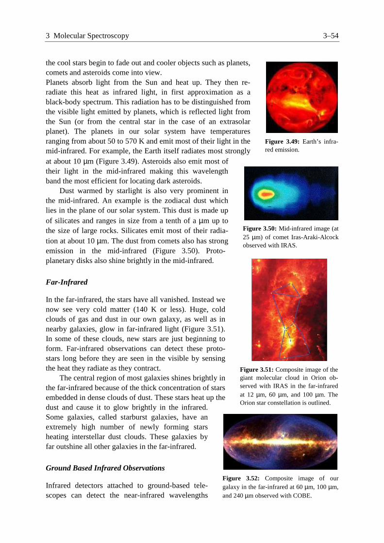
the cool stars begin to fade out and cooler objects such as planets, comets and asteroids come into view. Planets absorb light from the Sun and heat up. They then re-radiate this heat as infrared light, in first approximation as a black-body spectrum. This radiation has to be distinguished from the visible light emitted by planets, which is reflected light from the Sun (or from the central star in the case of an extrasolar planet). The planets in our solar system have temperatures ranging from about 50 to 570 K and emit most of their light in the mid-infrared. For example, the Earth itself radiates most strongly at about 10 µm (Figure 3.49). Asteroids also emit most of their light in the mid-infrared making this wavelength band the most efficient for locating dark asteroids.

Dust warmed by starlight is also very prominent in the mid-infrared. An example is the zodiacal dust which lies in the plane of our solar system. This dust is made up of silicates and ranges in size from a tenth of a µm up to the size of large rocks. Silicates emit most of their radia-tion at about 10 µm. The dust from comets also has strong emission in the mid-infrared (Figure 3.50). Proto-planetary disks also shine brightly in the mid-infrared.

Far-Infrared

In the far-infrared, the stars have all vanished. Instead we now see very cold matter (140 K or less). Huge, cold clouds of gas and dust in our own galaxy, as well as in nearby galaxies, glow in far-infrared light (Figure 3.51). In some of these clouds, new stars are just beginning to form. Far-infrared observations can detect these proto-stars long before they are seen in the visible by sensing the heat they radiate as they contract.

The central region of most galaxies shines brightly in the far-infrared because of the thick concentration of stars embedded in dense clouds of dust. These stars heat up the dust and cause it to glow brightly in the infrared. Some galaxies, called starburst galaxies, have an extremely high number of newly forming stars heating interstellar dust clouds. These galaxies by far outshine all other galaxies in the far-infrared.

Ground Based Infrared Observations

Infrared detectors attached to ground-based tele-scopes can detect the near-infrared wavelengths

Figure 3.49: Earth’s infra-red emission.

Figure 3.50: Mid-infrared image (at 25 µm) of comet Iras-Araki-Alcock observed with IRAS.

Figure 3.51: Composite image of the giant molecular cloud in Orion ob-served with IRAS in the far-infrared at 12 µm, 60 µm, and 100 µm. The Orion star constellation is outlined.

Figure 3.52: Composite image of our galaxy in the far-infrared at 60 µm, 100 µm, and 240 µm observed with COBE.


which make it through our atmosphere. The best location for ground based infrared observato-ries is on a high, dry mountain, above much of the water vapor which absorbs infrared radia-tion. At these high altitudes, we can study infrared bands up to about 35 µm.

The first infrared sky survey (at 2.2 µm) was conducted at the Mount Wilson Observatory (California, next to Los Angeles), where also data for the first infrared star catalogue was obtained. Nowadays, the largest group of infrared telescopes can be found on top of Mauna Kea (a dormant volcano) on Big Island, Hawaii. At an elevation of 4200 m, the Mauna Kea Observatory, which was founded in 1967, is well above much of the infrared absorbing water vapor.

High-Atmosphere Infrared Astronomy

It is best to get above as much of the atmosphere as possible to observe in the infrared. To do so, infrared detectors have been placed on balloons, rockets and airplanes, allowing us to study also mid- and far-infrared wavelengths. For example, infrared telescopes onboard aircraft such as the Kuiper Airborne Observatory were used to discover the rings of Uranus in 1977.

NASA and the German Aerospace Center (DLR) are currently developing jointly a new airborne observatory, the Stratospheric Observatory For Infrared Astronomy (SOFIA), an optical/infrared/sub-millimeter 2.7 m telescope mounted in a Boeing 747. It will observe in the range from 0.3 to 655 µm. In 2009 the aircraft is undergoing test flights at high altitude (the intended observing altitude is 12 km). The start of science operation is scheduled to 2011, though full capability will only be reached by 2014.

Infrared Astronomy from Space

Infrared space telescopes are not restricted by the transmission windows of Earth’s atmosphere. Furthermore, they can view a large area of the sky and observe regions for longer time periods than is possible with telescopes onboard balloons or aircrafts.

Infrared detectors have to be kept in an environment which is as cold as possible. The colder the environment, the more sensitive the instruments are to infrared light. Any surrounding heat will create infrared signals that can interfere with signals from space. This includes heat radiation from the instruments and telescope, from the atmosphere (for ground-based observatories), and from warmer objects in space like the Sun. To keep infrared detectors and instruments cold, cryogens such as liquid helium are used. The cryogen is usually contained in a chamber called a cryostat. Solar shields are also placed on infrared space telescopes to protect the instruments from the Sun’s heat.

The lifetime of an infrared space mission depends on how long the instruments can remain cold. Shortly after the cryogen (or coolant) runs out, the detectors will become useless and the data gathering portion of the mission will end. The relatively short lifetime of a few years is a major disadvantage of space missions.

In the following we list the most important infrared space telescopes, covering past and current missions as well as currently planned, future telescopes.


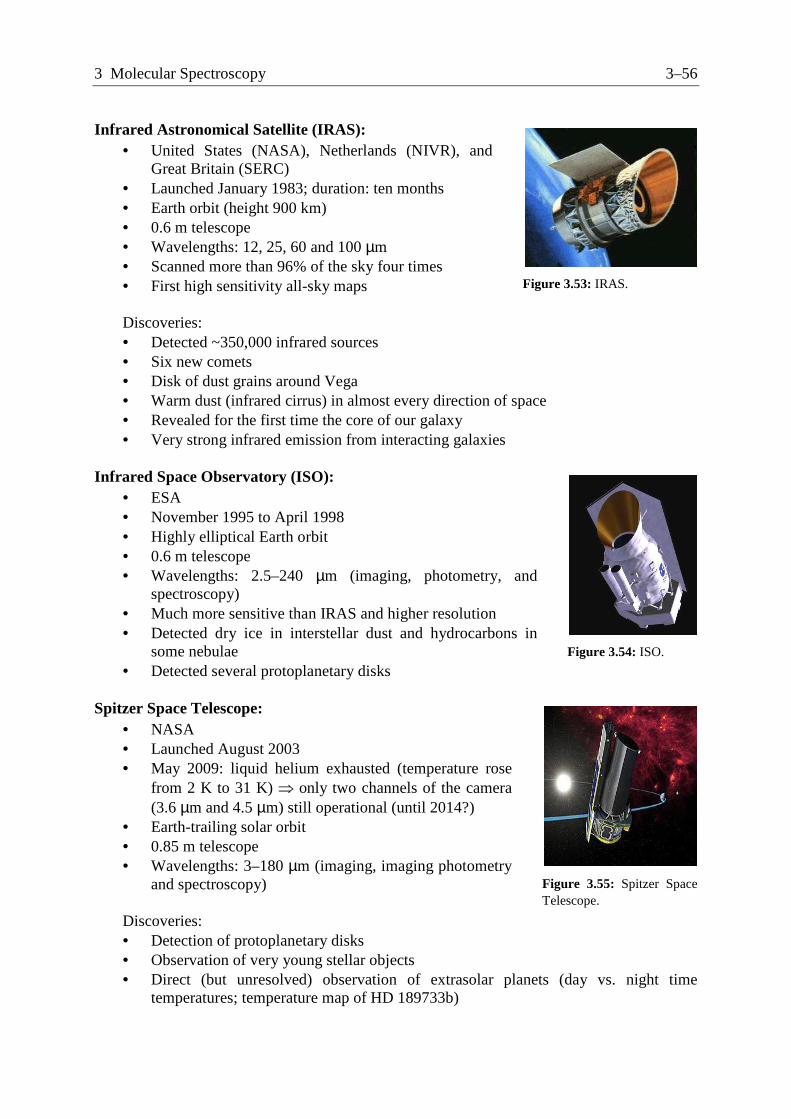
Infrared Astronomical Satellite (IRAS): • United States (NASA), Netherlands (NIVR), and

Great Britain (SERC) • Launched January 1983; duration: ten months • Earth orbit (height 900 km) • 0.6 m telescope • Wavelengths: 12, 25, 60 and 100 µm • Scanned more than 96% of the sky four times • First high sensitivity all-sky maps Discoveries: • Detected ~350,000 infrared sources • Six new comets • Disk of dust grains around Vega • Warm dust (infrared cirrus) in almost every direction of space • Revealed for the first time the core of our galaxy • Very strong infrared emission from interacting galaxies

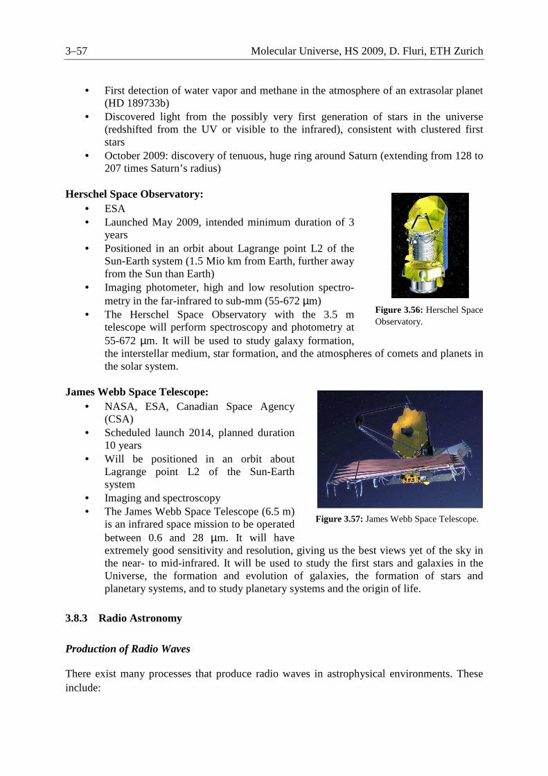
Infrared Space Observatory (ISO): • ESA • November 1995 to April 1998 • Highly elliptical Earth orbit • 0.6 m telescope • Wavelengths: 2.5–240 µm (imaging, photometry, and

spectroscopy) • Much more sensitive than IRAS and higher resolution • Detected dry ice in interstellar dust and hydrocarbons in

some nebulae • Detected several protoplanetary disks

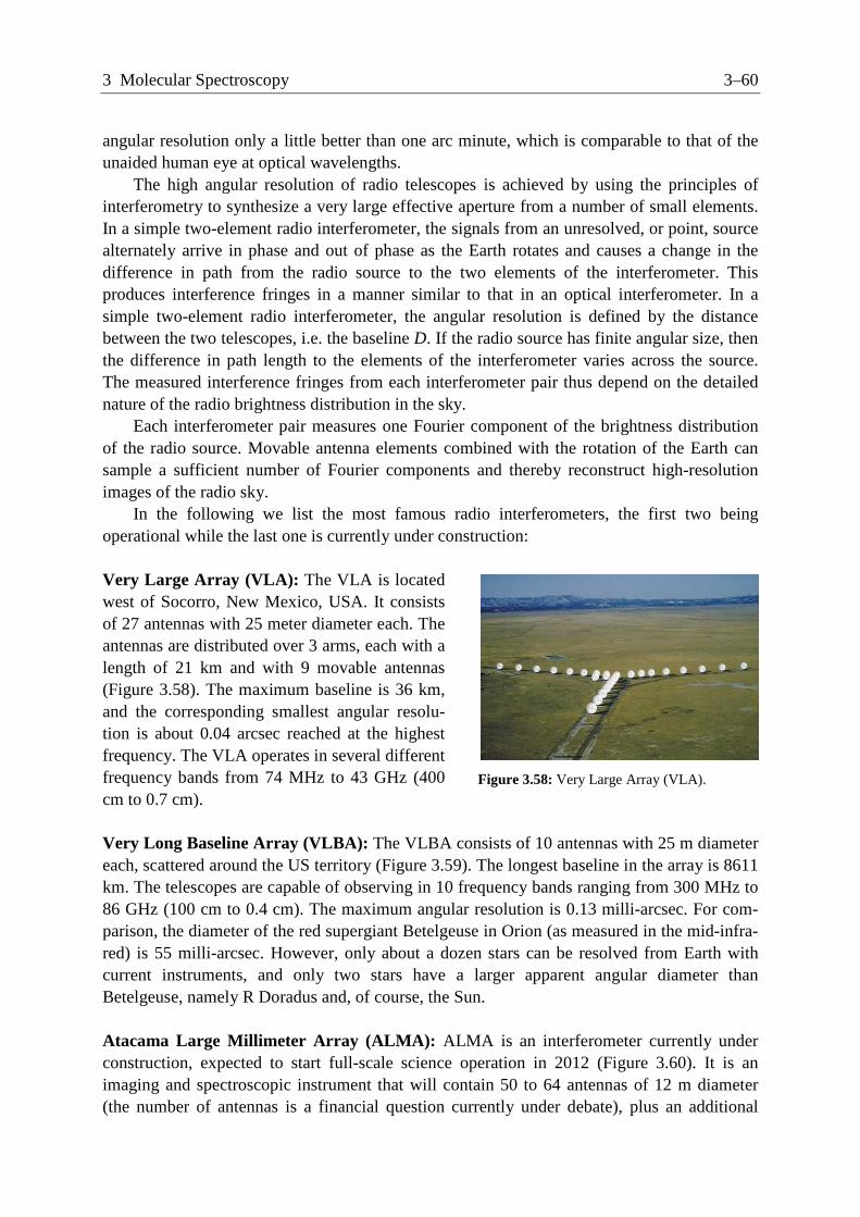
Spitzer Space Telescope:

• NASA • Launched August 2003 • May 2009: liquid helium exhausted (temperature rose

from 2 K to 31 K) ⇒ only two channels of the camera (3.6 µm and 4.5 µm) still operational (until 2014?)

• Earth-trailing solar orbit • 0.85 m telescope • Wavelengths: 3–180 µm (imaging, imaging photometry

and spectroscopy) Discoveries: • Detection of protoplanetary disks • Observation of very young stellar objects • Direct (but unresolved) observation of extrasolar planets (day vs. night time

temperatures; temperature map of HD 189733b)

Figure 3.53: IRAS.

Figure 3.54: ISO.

Figure 3.55: Spitzer Space Telescope.


• First detection of water vapor and methane in the atmosphere of an extrasolar planet (HD 189733b)

• Discovered light from the possibly very first generation of stars in the universe (redshifted from the UV or visible to the infrared), consistent with clustered first stars

• October 2009: discovery of tenuous, huge ring around Saturn (extending from 128 to 207 times Saturn’s radius)

Herschel Space Observatory: • ESA • Launched May 2009, intended minimum duration of 3

years • Positioned in an orbit about Lagrange point L2 of the

Sun-Earth system (1.5 Mio km from Earth, further away from the Sun than Earth)

• Imaging photometer, high and low resolution spectro-metry in the far-infrared to sub-mm (55-672 µm)

• The Herschel Space Observatory with the 3.5 m telescope will perform spectroscopy and photometry at 55-672 µm. It will be used to study galaxy formation, the interstellar medium, star formation, and the atmospheres of comets and planets in the solar system.

James Webb Space Telescope: • NASA, ESA, Canadian Space Agency

(CSA) • Scheduled launch 2014, planned duration

10 years • Will be positioned in an orbit about

Lagrange point L2 of the Sun-Earth system

• Imaging and spectroscopy • The James Webb Space Telescope (6.5 m)

is an infrared space mission to be operated between 0.6 and 28 µm. It will have extremely good sensitivity and resolution, giving us the best views yet of the sky in the near- to mid-infrared. It will be used to study the first stars and galaxies in the Universe, the formation and evolution of galaxies, the formation of stars and planetary systems, and to study planetary systems and the origin of life.

3.8.3 Radio Astronomy

Production of Radio Waves

There exist many processes that produce radio waves in astrophysical environments. These include:

Figure 3.56: Herschel Space Observatory.

Figure 3.57: James Webb Space Telescope.


• Spectral line radiation from atomic or molecular transitions that occur in the interstellar medium or in the gaseous envelopes around stars.

• Bremsstrahlung or thermal radiation from hot gas in the interstellar medium. • Synchrotron radiation from relativistic electrons in weak magnetic fields. • Pulsed radiation resulting from the rapid rotation of neutron stars surrounded by an

intense magnetic field and energetic electrons. Interestingly, radio astronomy is not only concerned with cold environments. Synchrotron radiation brings in an immediate cross-disciplinary contact between radio and high-energy astrophysics, a connection that might have been thought unlikely because of the low energies of radio photons. In fact, there is a high relevance of radio observations to high-energy phenomena since the radio and X-ray observations of active galactic nuclei and quasars have close relationships to one another.

Discoveries

Radio waves penetrate much of the gas and dust in space as well as the clouds of planetary atmospheres and pass through the terrestrial atmosphere with little distortion. Apart from different physical processes causing radio waves, this makes radio astronomy so valuable and complementary to optical astronomy since is allows us to observe objects that remain hidden to visible wavelengths. Nevertheless, optical observations are essential to understand what types of objects are the sources of radio emission, and to put radio observations into a physical and astrophysical context. Not surprisingly, this has led to important advances. We just mention here the most famous discoveries of radio astronomy:

• 1933: Karl Jansky first detected cosmic radio noise from the center of our galaxy

(resulting from synchrotron radiation) while investigating radio disturbances interfering with the transoceanic telephone service.

• 1940/50’s: Australian and British radio scientists located a number of discrete radio sources associated with old supernovae and active galaxies, which later became known as radio galaxies.

• 1963: Maarten Schmidt discovered quasars. • 1965: Arno A. Penzias and Robert W. Wilson detected the cosmic microwave back-

ground radiation at a temperature of 3 K. • 1967: Jocelyn Bell and Antony Hewish discovered pulsars, rapidly rotating magnetic

neutron stars. • More than 100 different molecules are detected in the space, including familiar

chemical compounds like water vapor, formaldehyde, ammonia, methanol, ethanol, and carbon dioxide.

Radio Bands

Radio waves have wavelengths longer than about 1 mm (300 GHz). For wavelengths in the range 1 cm – 20 cm Earth’s atmosphere, in particular the ionosphere, introduce only minor distortion to incident radiation. At wavelengths below about 1 cm (30 GHz) absorption in the


atmosphere becomes increasingly critical, and observations from the ground are possible only in a few specific wavelength bands that are relatively free of atmospheric absorption. At wavelengths longer than 20 cm irregularities in the ionosphere distort incoming signals. This causes a phenomenon known as scintillation, which is analogous to the twinkling of stars seen at optical wavelengths. The absorption of cosmic radio waves by the ionosphere becomes more important as the wavelength increases. At wavelengths longer than about 10 m (30 MHz), the ionosphere becomes opaque to incident signals. Therefore, radio observations of cosmic sources at these wavelengths are difficult from ground-based radio telescopes.

Radio Telescopes

The instrumental methods of the radio astronomer often appear to be quite different from those of the optical astronomer. The distinguishing feature of a radio telescope is that the radiation energy gathered by the parabolic antenna is not measured immediately, a process known as detection in radio terminology. Instead, the radiation is amplified and manipulated coherently, preserving its wave-like character, before it is finally detected. It is crucial to cool the amplifier cryogenically to reduce the internal noise as much as possible and to increase the sensitivity of the instrument. The instrumental goals of the radio astronomer, i.e. obtaining a larger collecting area, greater angular resolution, and more sensitive detectors, are otherwise the same as they are for all astrophysical disciplines.

Radio telescopes are used to measure broad-bandwidth continuum radiation as well as spectroscopic features due to atomic and molecular lines found in the radio spectrum of astrophysical objects. In early radio telescopes, spectroscopic observations were made by tuning a receiver across a sufficiently large frequency range to cover the various frequencies of interest. This procedure, however, was extremely time-consuming and greatly restricted observations. Modern radio telescopes observe simultaneously at a large number of frequencies by dividing the signals up into as many as several thousand separate frequency channels that may range over a total bandwidth of tens to hundreds of megahertz.

The most straightforward type of radio spectrometer employs a large number of filters, each tuned to a separate frequency and followed by a separate detector to produce a multi-channel, or multi-frequency, receiver. Alternatively, a single broad-bandwidth signal may be converted into digital form and analyzed by the mathematical process of autocorrelation and Fourier transformation. In order to detect faint signals, the receiver output is often averaged over periods of up to several hours to reduce the effect of noise generated in the receiver.

Radio Interferometry

The angular resolution θ of a telescope depends on the wavelength of observations λ and the size of the dish D and can be approximated by

.D

λθ = (3.97)

Because radio telescopes operate at much longer wavelengths than optical telescopes, radio telescopes must be much larger than optical telescopes to achieve the same angular resolution. Yet, even the largest antennas, when used at their shortest operating wavelength, have an


angular resolution only a little better than one arc minute, which is comparable to that of the unaided human eye at optical wavelengths.

The high angular resolution of radio telescopes is achieved by using the principles of interferometry to synthesize a very large effective aperture from a number of small elements. In a simple two-element radio interferometer, the signals from an unresolved, or point, source alternately arrive in phase and out of phase as the Earth rotates and causes a change in the difference in path from the radio source to the two elements of the interferometer. This produces interference fringes in a manner similar to that in an optical interferometer. In a simple two-element radio interferometer, the angular resolution is defined by the distance between the two telescopes, i.e. the baseline D. If the radio source has finite angular size, then the difference in path length to the elements of the interferometer varies across the source. The measured interference fringes from each interferometer pair thus depend on the detailed nature of the radio brightness distribution in the sky.

Each interferometer pair measures one Fourier component of the brightness distribution of the radio source. Movable antenna elements combined with the rotation of the Earth can sample a sufficient number of Fourier components and thereby reconstruct high-resolution images of the radio sky.

In the following we list the most famous radio interferometers, the first two being operational while the last one is currently under construction:

Very Large Array (VLA): The VLA is located west of Socorro, New Mexico, USA. It consists of 27 antennas with 25 meter diameter each. The antennas are distributed over 3 arms, each with a length of 21 km and with 9 movable antennas (Figure 3.58). The maximum baseline is 36 km, and the corresponding smallest angular resolu-tion is about 0.04 arcsec reached at the highest frequency. The VLA operates in several different frequency bands from 74 MHz to 43 GHz (400 cm to 0.7 cm).

Very Long Baseline Array (VLBA): The VLBA consists of 10 antennas with 25 m diameter each, scattered around the US territory (Figure 3.59). The longest baseline in the array is 8611 km. The telescopes are capable of observing in 10 frequency bands ranging from 300 MHz to 86 GHz (100 cm to 0.4 cm). The maximum angular resolution is 0.13 milli-arcsec. For com-parison, the diameter of the red supergiant Betelgeuse in Orion (as measured in the mid-infra-red) is 55 milli-arcsec. However, only about a dozen stars can be resolved from Earth with current instruments, and only two stars have a larger apparent angular diameter than Betelgeuse, namely R Doradus and, of course, the Sun.

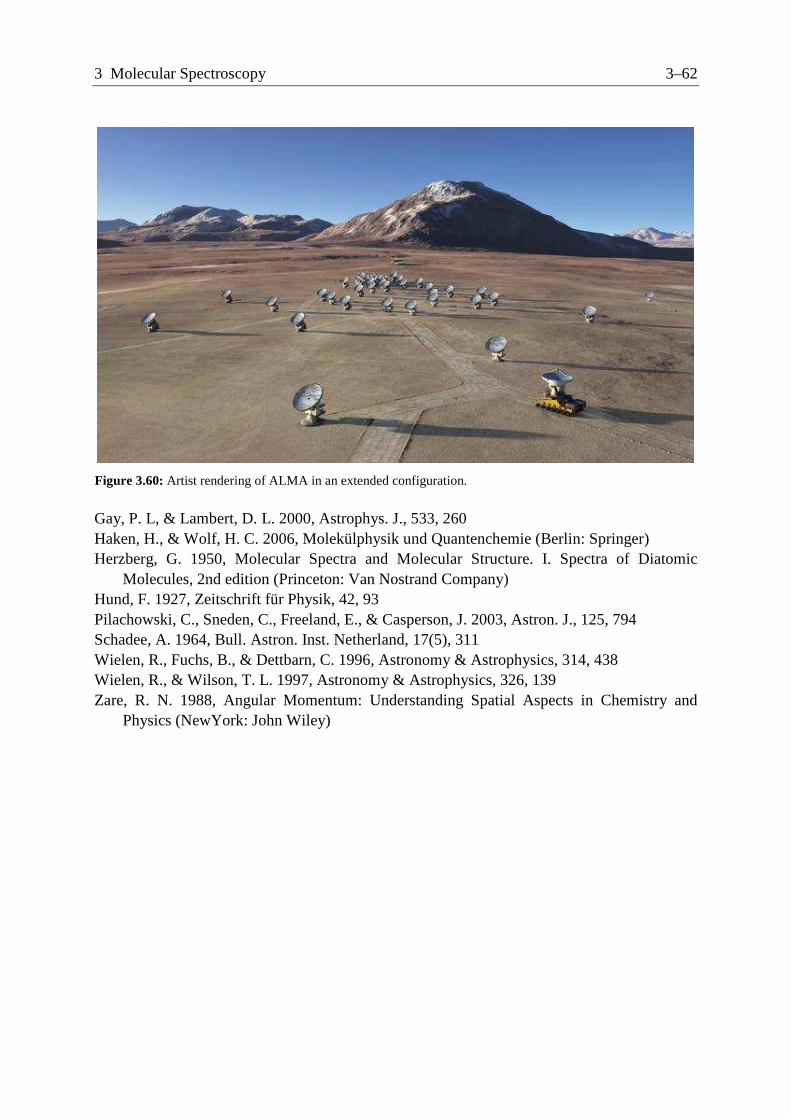
Atacama Large Millimeter Array (ALMA): ALMA is an interferometer currently under construction, expected to start full-scale science operation in 2012 (Figure 3.60). It is an imaging and spectroscopic instrument that will contain 50 to 64 antennas of 12 m diameter (the number of antennas is a financial question currently under debate), plus an additional

Figure 3.58: Very Large Array (VLA).


compact array of four 12 m antennas and twelve 7 m antennas. The array is located Llano de Chajnantor Observatory in the Atacama Desert in northern Chile at an altitude of 5000 m. The 12 m antennas will have reconfigurable baselines ranging from 150 m to 16 km. The instruments can observe wavelengths in the sub-millimeter to millimeter range and operate in all atmospheric windows between 350 µm and 10 mm, and thus cover the short wavelength end of radio waves. ALMA can reach a spatial resolution of 10 milli-arcsec and will become the largest and most sensitive instrument in the sub-millimeter and millimeter range. The science goals of ALMA include studying the first stars and galaxies in the universe by imaging the redshifted dust continuum emission at epochs as early as z = 10, studying the physical and chemical conditions of protoplanetary disks, young stars, and circumstellar shells and envelopes around evolved stars, novae and supernovae, and probing the interstellar medium in different galactic environments.

References

Ayres, T. R., Plymate, C., & Keller, C. U. 2006, Astrophys. J. Suppl. Ser., 165, 618 Berdyugina, S. V., Stenflo, J. O, & Gandorfer, A. 2002, Astronomy & Astrophysics, 388,

1062 Bernath, P. F. 2005, Spectra of Atoms and Molecules (Oxford: Oxford Univ. Press.) Born, M, & Oppenheimer, J. R. 1927, Ann. Phys., 84, 457

Figure 3.59: The ten instruments belonging to the VLBA.


Gay, P. L, & Lambert, D. L. 2000, Astrophys. J., 533, 260 Haken, H., & Wolf, H. C. 2006, Molekülphysik und Quantenchemie (Berlin: Springer) Herzberg, G. 1950, Molecular Spectra and Molecular Structure. I. Spectra of Diatomic

Molecules, 2nd edition (Princeton: Van Nostrand Company) Hund, F. 1927, Zeitschrift für Physik, 42, 93 Pilachowski, C., Sneden, C., Freeland, E., & Casperson, J. 2003, Astron. J., 125, 794 Schadee, A. 1964, Bull. Astron. Inst. Netherland, 17(5), 311 Wielen, R., Fuchs, B., & Dettbarn, C. 1996, Astronomy & Astrophysics, 314, 438 Wielen, R., & Wilson, T. L. 1997, Astronomy & Astrophysics, 326, 139 Zare, R. N. 1988, Angular Momentum: Understanding Spatial Aspects in Chemistry and

Physics (NewYork: John Wiley)

Figure 3.60: Artist rendering of ALMA in an extended configuration.

3.7 Isotope Effect - Homepage – Institute for Particle ... · Figure 3.45: Comparison of the...

Documents

Transcript of 3.7 Isotope Effect - Homepage – Institute for Particle ... · Figure 3.45: Comparison of the...