14 April 2016

Dr. John Hedengren

350 CB Brigham Young University

Provo, UT 84606

Dr. Hedengren:

Compressors in gas pipelines are designed to maintain pressure and flow despite many flow

disturbances that can occur during transport. The most common control implementation for gas

compressors utilizes a recycle bleed stream that essentially recycles a portion of the pressurized stream

in order to maintain a pressure or flow set point. This process wastes energy and shows a slow response

time because of valve dynamics. A. Cortinovis et.al. developed a linear MPC controller to accomplish the

same control objective but instead manipulates the compressor driver torque in order to control the

discharge pressure and flow rate. Their study showed that controller settling time decreased by about

50% using the MPC.

Because gas pipelines utilize many compressors along the length of the supply line, it is desirable to

develop a reliable, energy efficient control scheme that can achieve anti-surge and process control for

gas compressors in series. This work explores a linear MPC to control a system of two compressors in

series. We extend the model developed by A. Cortinovis et.al., simulate the model in Simulink, and

extract a linear state-space model for use in the linear MPC. The linear MPC maintains a pressure set

point in each compressor, while manipulating driver torque to achieve the set point. Currently, the MPC

works in tandem with a separate PI controller, which acts as the recycle anti-surge control utilized in

current practices. The set point tracking and disturbance rejection ability of the controller are then

tested to show the controller performance.

This linear MPC is a first-step towards implementing this controller in a physical plant. Future work will

combine the anti-surge control together with the pressure tracking MPC in a non-linear MPC. This will

allow for a more robust controller that can then be tested on an experimental pilot system.

Sincerely,

Aaron Bush

Brandon Hillyard

Highlights:

Linear MPC for a gas compressor system is extended for use with two gas compressors in series

A first-principles model of the two compressor system is simulated in Simulink

A state-space model is extracted from the full model and implemented in a linear MPC in

tandem with a recycle valve PI controller

The controller responds quickly to disturbances and set point changes, achieving the desired

anti-surge control

Competition between the two separate controllers causes unexpected oscillations and loss of

control; future work will combine both controllers into one nonlinear model predictive control

scheme

LINEAR MODEL PREDICTIVE CONTROL AND ANTI-SURGE CONTROL FOR CENTRIFUGAL

GAS COMPRESSORS IN SERIES

By

Aaron Bush

Brandon Hillyard

14 April 2016

Contents Figures and Tables ........................................................................................................................................ 1

Introduction .................................................................................................................................................. 2

Literature Review .......................................................................................................................................... 2

Theory ........................................................................................................................................................... 3

Methods ........................................................................................................................................................ 3

Process flow diagram ................................................................................................................................ 3

Inputs and Outputs ................................................................................................................................... 4

Model Equations ....................................................................................................................................... 4

Simulation Results ......................................................................................................................................... 5

Linear Model for MPC ............................................................................................................................... 5

Model Predictive Controller .......................................................................................................................... 5

Objective Function .................................................................................................................................... 6

MPC Configuration .................................................................................................................................... 6

Dynamic Optimization Results and Discussion ............................................................................................. 6

Set Point tracking ...................................................................................................................................... 7

Disturbance Rejection ............................................................................................................................... 8

Anti-surge control ..................................................................................................................................... 9

Sensitivity Analysis .................................................................................................................................... 9

Conclusions and Recommendations ........................................................................................................... 10

Acknowledgments ....................................................................................................................................... 10

References .................................................................................................................................................. 10

Appendix ..................................................................................................................................................... 11

1

Figures and Tables Table 1 Sensitivity Analysis performed in APMonitor .................................................................................. 9

Figure 1 - Compressor map showing the optimal operating point ............................................................... 3

Figure 2 - Process flow diagram of two gas compressors in series with recycle and an intermediate tank 4

Figure 3 L1-norm objective function ............................................................................................................. 6

Figure 5 Pressure Set Point response of Compressor 1 ................................................................................ 7

Figure 4 Pressure Set Point response of Compressor 2 ................................................................................ 7

Figure 6 Disturbance Rejection Test - Discharge Pressure of Compressor 1 ................................................ 8

Figure 7 Disturbance Rejection Test - Discharge Pressure of Compressor 2 ................................................ 8

Figure 8 Anti-Surge controller response. The solid line represents the surge line, while the dotted line

represents the best operating line. .............................................................................................................. 9

2

LINEAR MODEL PREDICTIVE CONTROL AND ANTI-SURGE CONTROL FOR CENTRIFUGAL GAS

COMPRESSORS IN SERIES

Introduction Compressors in gas pipelines are designed to maintain pressure and flow despite many flow

disturbances that can occur during transport. Conventional control schemes employed in gas

compressor systems include a recycle “bleed” stream that maintains a pressure set point by recycling

gas. This set up is an effective means of eliminating compressor surge, a condition of flow instability that

arises when the ratio of downstream to upstream pressure exceeds an amount unacceptable for the

flow rate. However, because the recycle stream essentially wastes energy and money used to pressurize

gas in the first place, this set up is not an ideal control method for anti-surge, especially in a situation

where two compressors are linked in series.

One method developed in a work by A. Cortinovis et.al. explores the use of linear model predictive

control (MPC) to manipulate the driver torque of a compressor linked to a variable speed drive (VSD) in

order to reduce the speed of the compressor and thus more effectively control the compressor output.

The results of that study show that the VSD responds more rapidly than a recycle control valve, and

allows for a more efficient compressor set up.

The purpose of this work is to extend the first-principles model developed by A. Cortinovis et.al. for two

compressors in series. The model is simulated using step responses to show the behavior of the system.

A linear state space model is then extracted for use with a linear MPC which manipulates the driver

torque of the two compressors to maintain discharge pressure set points for the system. The MPC is

implemented in tandem with a standard anti-surge recycle controller as a first step in the controller

design to improve the controller performance. The performance of the controller is then discussed, and

future work is laid forth.

Literature Review The work performed by A. Cortinovis et.al. develops an improved method for controlling gas

compressors and eliminating surge than the current industry practice. This method relies on a linear

model predictive controller for anti-surge and process control, similar to the method explored in this

work. A first principles model relating pressures, flow rates, and valve positions serves as the basis for

the controller model, which is linearized and discretized at each time step before implementation in the

solver. The model dynamic and static parameters are validated using an experimental test rig, after

which the controller performance is compared with a traditional PI recycle controller. The MPC

compared to the PI controller reduces settling time by 50%, and the distance to surge by up to 11%,

exhibiting the value of the MPC controller for this application.

This study builds upon the work established by A. Cortinovis et.al. by applying the linear MPC to two

compressors in series. The same parameters developed in the single compressor model are extended

for use in the two compressor model. Because the nonlinearities that exist in the single compressor

system are multiplied when two compressors are coupled together, this work will explore whether a

linear MPC set up is a desirable control scheme. The MPC is tested in order to determine the set point

3

tracking and disturbance rejection ability of the system. Failure of the controller in these tests may

indicate that a nonlinear MPC is a more favorable solution to the serial compressor model.

Theory Figure 1 graphically represents the operating points of a gas compressor. The vertical axis represents the

pressure ratio (Π) of the compressor, while the horizontal axis represents the mass flow rate of the

compressor 𝑞𝑐. Optimal operation occurs along a line of peak efficiency (represented by curved lines)

while optimizing the distance (SD) from the surge line (SL) and the choke line (CL). Crossing SL can lead

to serious damage in the compressor and reverse flow conditions. To tighten control further and

remove the possibility of crossing the SL, a surge control line (SCL) may be set a specified distance from

the SL. It is desired to maintain operation an optimal distance from SCL and CL to avoid surging and

deliver flow at the most efficient conditions.

Methods This section details the first principle equations upon which a simulation of the model is built in

Simulink. The equations and parameters used in this model are identical to those used in A. Cortinovis

et.al., and are simply duplicated for the second compressor and linked together with an intermediate

tank to decouple the systems. The process is described, and the equations used to model the system in

Simulink are set forth.

Process flow diagram Figure 2 shows a schematic of the two compressors in series linked together with an intermediate tank.

Air flow to the suction side of compressor 1 is regulated by a control valve with flow rate 𝑞𝑠, as well as a

suction tank, 𝑉𝑠. The compressor operates with a rotational speed 𝜔 and compresses the gas with a flow

rate from the compressor of 𝑞𝑐. The gas enters a discharge tank 𝑉𝑑 at a pressure of 𝑝𝑑. An intermediate

tank with pressure 𝑃𝑖 connects the two compressors. Two control valves regulate the flow in and out of

this tank, and subsequently the flow into the next compressor.

FIGURE 1 - COMPRESSOR MAP SHOWING THE OPTIMAL

OPERATING POINT

4

Inputs and Outputs The system as shown in Figure 2 is modeled in Simulink in order to characterize the input to output

relationships of the model. Each compressor system takes the suction valve openings, recycle rates, and

motor torque speeds of each compressor as inputs to the system, and outputs a pressure and

compressor mass flow rate. The intermediate tank 𝑃𝑖 serves as a buffer between the two compressor

systems to effectively decouple the compressors and maximize control of the system. The output

pressure of the intermediate tank is based on the mass flow out of the first compressor (𝑞𝑑) and mass

flow into the second compressor (𝑞𝑠). The size of the intermediate tank determines how quickly changes

will occur to one compressor based on changes in operation from the other compressor. For the

purposes of this exercise, the volume of this tank is chosen to be the same as the suction and discharge

tanks shown in Figure 2.

Model Equations The system is modeled using dynamic equations to represent the change in pressure as a function of

mass flow rate across the compressors. The equations are equivalent to those presented in the work by

A. Cortinovis et.al. and are listed for reference. The gas flow rates are functions of the valve position (𝑢),

pressure (𝑝), and ambient pressure (𝑝𝑎), and are based on the simplified Bernoulli throttle equation.

𝑞𝑠 = 𝑞𝑠(𝑢𝑖𝑛, 𝑝𝑠 , 𝑝𝑎) (1)

𝑞𝑟 = 𝑞𝑟(𝑢𝑟, 𝑝𝑠 , 𝑝𝑑) (2)

𝑞𝑑 = 𝑞𝑑(𝑢𝑜𝑢𝑡, 𝑝𝑎 , 𝑝𝑑) (3)

The dynamic pressure relationships are given by the following equations, derived from a mass balance

on the suction, discharge, and intermediate tank (where 𝑎 is the speed of sound and 𝑉 is the volume of

the tank):

𝑑𝑝𝑠

𝑑𝑡=

𝑎2

𝑉𝑠

(𝑞𝑠 + 𝑞𝑟 + 𝑞𝑐) (4)

FIGURE 2 - PROCESS FLOW DIAGRAM OF TWO GAS COMPRESSORS IN SERIES WITH RECYCLE AND AN INTERMEDIATE

TANK

5

𝑑𝑝𝑑

𝑑𝑡=

𝑎2

𝑉𝑑

(𝑞𝑐 − 𝑞𝑟 − 𝑞𝑑) (5)

𝑑𝑝𝑖𝑛𝑡

𝑑𝑡=

𝑎2

𝑉𝑖𝑛𝑡

(𝑞𝑑1 − 𝑞𝑠2) (6)

A mass balance on the compressor yields the following relationship for the compressor flow rate,

𝑑𝑞𝑐

𝑑𝑡=

𝐴

𝑙𝑐

(Π𝑠𝑠(�⃗�, 𝜔, 𝑞𝑐)𝑝𝑠 − 𝑝𝑑) (7)

where 𝐴 is the piping cross section, 𝑙𝑐 the duct length, and Π𝑠𝑠 is a fitted polynomial map for the steady

state pressure ratio.1 Finally, an equation relating the variation of the compressor speed with respect to

torque is shown in Equation 8, where 𝐽 is the inertia of the system, 𝜏𝑑 is the driver torque input to the

system, 𝜏𝑐 is the torque from the air compression fitted to a steady state map with parameters 𝛽, as

described in detail in A. Cortinovis et.al.

𝑑𝜔

𝑑𝑡=

1

𝐽(𝜏𝑑 − 𝑇𝑐(𝛽, 𝜔, 𝑞𝑐)) (8)

Simulation Results A model of two compressors in series is created utilizing the single compressor first principles model

developed by A. Cortinovis et.al. This compressor series model is implemented using Simulink in Matlab

2015b. In order to develop a linear state space model it is necessary to perform step tests from steady

state operation. Steady state operation is determined by the intermediate tank pressure. In order to

achieve steady state, torque of compressor 1 is adjusted until a constant pressure is observed in the

intermediate tank. Step tests are then performed by changing torque on each compressor, and the

response in outlet pressure and flow is recorded. The step value and step response are then used in

developing a linear state space model for use in the MPC.

Linear Model for MPC The steady-state first principles is then linearized to a form compatible with the linear MPC. The inputs

of this linear model are the driver torques of compressor 1 and 2 respectively, and the outputs are the

mass flow rates and discharge pressures of each compressor, as well as the pressure of the intermediate

tank. The linear model extracted from the system consists of 2nd-4th order state space models. The full

models are shown in the Appendix. The two compressors are coupled, despite the presence of the

intermediate tank, so each output variable is affected by both the torque of compressor 1 and

compressor 2.

Model Predictive Controller The model predictive controller implemented in this process utilizes the linear state space model, as

well as the full process model developed previously to perform the anti-surge and discharge pressure

control. Included in the process model is the anti-surge recycle controller that utilizes the recycle line to

assist with the anti-surge control.

6

Objective Function The anti-surge controller is a replicate of the controller produced in the work by A. Cortinovis et.al. The

same controller is implemented for both compressors, and is designed to work in tandem with the linear

MPC to control surge in the system. This controller manipulates recycle valve position in order to control

the location of the operating point and maintain an optimal distance from the surge line.

The objective of the linear MPC is to manipulate torque on each of the compressor drives to maintain

discharge pressure set points. This is accomplished using an L1-norm objective function using the form

described below in Figure 3. This objective allows the user to specify a trajectory for the controlled

variable, as well as a high and low set point to bound the targeted controller response. The slack

variable formulation of the error is desirable as it formulates the error as soft constraints, and thus

enables a smoother controller action.

𝑚𝑖𝑛ϕ = whi𝑇 𝑒ℎ𝑖 + 𝑤𝑙𝑜

𝑇 𝑒𝑙𝑜 + 𝑦𝑇𝑐𝑦 + 𝑢𝑇𝑐𝑢 + Δ𝑢𝑇𝑐Δ𝑢

𝑚𝑖𝑛ϕ = whi𝑇 𝑒ℎ𝑖 + 𝑤𝑙𝑜

𝑇 𝑒𝑙𝑜 + 𝑦𝑇𝑐𝑦 + 𝑢𝑇𝑐𝑢 + Δ𝑢𝑇𝑐Δ𝑢

𝑥, 𝑦, 𝑢

s.t. 0 = 𝑓 (𝑑𝑥

𝑑𝑡, 𝑥, 𝑦, 𝑝, 𝑑, 𝑢)

0 = 𝑔(𝑥, 𝑦, 𝑝, 𝑑, 𝑢) 0 ≤ ℎ(𝑥, 𝑦, 𝑝, 𝑑, 𝑢)

𝜏𝑐

𝑑𝑦𝑡,ℎ𝑖

𝑑𝑡+ 𝑦𝑡,ℎ𝑖 = 𝑠𝑝ℎ𝑖

𝜏𝑐

𝑑𝑦𝑡,𝑙𝑜

𝑑𝑡+ 𝑦𝑡,𝑙𝑜 = 𝑠𝑝𝑙𝑜

𝑒ℎ𝑖 ≥ 𝑦 − 𝑦𝑡,ℎ𝑖

𝑒𝑙𝑜 ≥ 𝑦𝑡,𝑙𝑜 − 𝑦

FIGURE 3 L1-NORM OBJECTIVE FUNCTION

MPC Configuration The linear MPC uses the APOPT solver in APMonitor to solve the objective function, and uses bias

updating from the full process model to update the model at each step in the time horizon. A predictive

time horizon of 5 seconds ensures that the controller fully experiences the dynamics of the system and

incorporates that into the control actions. The full code for the MPC controller and the linear state-

space model is shown in the Appendix.

Several tuning constraints are implemented in the MPC in order to improve control and reflect the limits

of the system. To improve controllability, an error band of +/-100 Pa is set around the set point, and is

coded as a trajectory that re-centers after each controller cycle. Allowing the set point trajectory to re-

center gives the controller greater freedom when disturbances occur or when the set point is adjusted

during operation. A physical constraint on the system is the amount the torque can change in each cycle

period. The torque can experience a maximum deviation of +/- 0.1 units per controller cycle (50 ms),

and is coded in as a hard constraint to the controller. These tuning parameters help to make the

controller more robust and able to reach the control objective.

Dynamic Optimization Results and Discussion This section shows the results of the linear MPC implemented with bias updating from the first-

principles model of the two compressors in series. The results show how pressure is able to be

7

controlled by the linear MPC, and that surge is minimized through the performance of the anti-surge

controller. A discussion on the disturbance rejection and set-point tracking ability of the controller is

included. And finally, a sensitivity analysis is performed to show the steady-state and dynamic

relationships between the manipulated variables and the controlled variables.

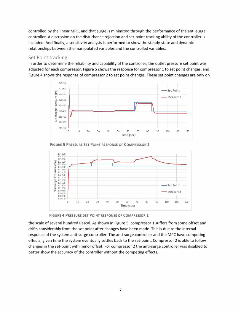
Set Point tracking In order to determine the reliability and capability of the controller, the outlet pressure set point was

adjusted for each compressor. Figure 5 shows the response for compressor 1 to set point changes, and

Figure 4 shows the response of compressor 2 to set point changes. These set point changes are only on

the scale of several hundred Pascal. As shown in Figure 5, compressor 1 suffers from some offset and

drifts considerably from the set point after changes have been made. This is due to the internal

response of the system anti-surge controller. The anti-surge controller and the MPC have competing

effects, given time the system eventually settles back to the set-point. Compressor 2 is able to follow

changes in the set-point with minor offset. For compressor 2 the anti-surge controller was disabled to

better show the accuracy of the controller without the competing effects.

FIGURE 4 PRESSURE SET POINT RESPONSE OF COMPRESSOR 1

FIGURE 5 PRESSURE SET POINT RESPONSE OF COMPRESSOR 2

8

Disturbance Rejection The system is also analyzed to determine the set point tracking ability of the controller. Disturbances are

introduced in the form of outlet valve changes for both of the compressor systems. The outflow valve

for compressor 1 was constricted from 0.45 to 0.29 after 10 seconds, and the outflow valve for

compressor 2 was constricted from 0.45 to 0.35 after 40 seconds. The results of the controller

performance are shown below in Figure 6 and Figure 7. The controller functions really well for the first

40 seconds of simulation time. It handles the first disturbance well, although some offset in the outlet

pressure of compressor 1 remains. After the outflow is constricted in compressor 2, the controller

gradually brings the discharge pressure of compressor 2 back under control by decreasing the torque of

both compressors. By the time discharge pressure 2 is under control, the pressure of compressor 1 has

drifted far below the set point, and is unable to recover.

Despite this, the controller seems to perform with little oscillation and with a very rapid response time,

much like the MPC developed in the single compressor plant by A. Cortinovis et.al. In addition, further

tests show that given more time, the pressure of compressor 1 is actually able to slowly recover back to

the set point.

The unexpected performance of the controller after the 40 second mark is partially explained by the fact

that changing the valve position moves the system outside the operating region that the linear MPC is

designed for. Another possible explanation is that there is some competition between the anti-surge

recycle controller and the MPC. Because the anti-surge controller is a Simulink based model, and the

MPC is written in APMonitor using a linearized form of the model, there’s no easy way to prioritize the

FIGURE 6 DISTURBANCE REJECTION TEST - DISCHARGE PRESSURE OF COMPRESSOR 1

FIGURE 7 DISTURBANCE REJECTION TEST - DISCHARGE PRESSURE OF COMPRESSOR 2

9

two control objectives, and the competing objectives drive the system away from the pressure set

points. This problem can be addressed by adapting the first principles Simulink model to a form that

works in APMonitor, which would allow the controller to be designed as a nonlinear MPC, and would

also streamline the simulation and bias updating of the controller.

Anti-surge control Both the set-point tracking and disturbance rejection tests show that the anti-surge objectives are able

to be met. The figures below show the compressor maps, with the leftmost red line representing the

surge line, the dotted line the best operating line, and the gold line the actual path that the compressor

followed over the sample time. The first compressor approaches surge at one point, but the anti-surge

controller turns on and drives the system back to the best operating line. The second compressor

system doesn’t operate anywhere near the surge line for a majority of the sample time, and only begins

to approach surge towards the end of the run. The anti-surge performance of the controller functions as

expected, due mostly to the fact that the recycle valve PI controller works in tandem with the MPC

controller. As mentioned previously, the performance of the MPC controller overall could be increased

by implementing the anti-surge control in the MPC rather than as a separate controller.

Sensitivity Analysis Table 1 below shows the results of the sensitivity analysis. It appears that neither of the compressor

flows vary much with torque manipulations. The discharge pressure of compressor 1 is affected by

torque 1, and inversely affected by torque 2. The discharge pressure of compressor 2 is affected very

little by torque 1, due mostly to the intermediate tank that separates the 2 compressor systems and

decouples them.

TABLE 1 SENSITIVITY ANALYSIS PERFORMED IN APMONITOR

FIGURE 8 ANTI-SURGE CONTROLLER RESPONSE. THE SOLID LINE REPRESENTS THE SURGE LINE, WHILE

THE DOTTED LINE REPRESENTS THE BEST OPERATING LINE.

10

Conclusions and Recommendations As shown in the disturbance rejection and set point tracking figures, the system can drift considerably

from the set point. The root cause of the drifting value is due to the inherent nonlinearity of the system.

The controller implemented is a linear model predictive controller, and any significant deviation from

the steady state values will result in inaccurate predictions. Recommended future work includes

developing a nonlinear MPC that integrates anti-surge and pressure set point control. This would not

only increase the set point tracking and disturbance rejection performance of the controller, but would

allow for a faster solve time on the computer. This is a recommended step before this controller is

implemented in a physical pilot system and validated with experimental data.

Acknowledgments The authors would like to thank Dr. Mehmet Mercangöz, as well as Dr. John Hedengren for their

continual help and mentorship throughout the project.

References 1. Cortinovis, A., Ferreau, H., Lewandowski, D., & Mercangöz, M. (2015). Experimental evaluation

of MPC-based anti-surge and process control for electric driven centrifugal gas compressors.

Journal of Process Control, 34, 13-25. doi:10.1016/j.jprocont.2015.07.001

11

Appendix State Space Model 1 – Compressor 1 flow

Torque 1 states [�̇�1] = 𝐴[𝑥1] + 𝐵[𝜏1]

Torque 2 states [�̇�2] = 𝐶[𝑥2] + 𝐷[𝜏2]

Compressor 1 flow [𝑞1] = 𝐸[𝑥1] + 𝐹[𝑥2] + 𝑞1,0

𝐴 = [

−0.1216 −0.2787 −0.1963 0.1248−0.1554 −0.5764 −0.6972 1.3509

0.1244 0.0656 −1.1303 10.97980.5790 1.1591 −5.3835 −2.8584

]

𝐵 = [0.0652 0.3301 2.3957 −2.0993]

𝐶 = [−0.0322 −0.0608−0.0106 −0.1002

]

𝐷 = [0 −0.0015]

𝐸 = [0.1995 −0.0024 −0.0016 −0.0005]

𝐹 = [0.2426 −0.0008]

𝑞1,0 = 0.594

State Space Model 2 – Compressor 2 flow

Torque 1 states [�̇�1] = 𝐴[𝑥1] + 𝐵[𝜏1]

Torque 2 states [�̇�2] = 𝐶[𝑥2] + 𝐷[𝜏2]

Compressor 2 flow [𝑞2] = 𝐸[𝑥1] + 𝐹[𝑥2] + 𝑞2,0

𝐴 = [

−0.1181 −0.2726 −0.9155 0.6859−0.1317 −0.2478 −3.5097 0.8864−0.4582 4.3268 −0.4612 0.18650.2484 −6.0631 1.4289 −7.3154

]

𝐵 = [0.0161 −0.0073 −0.0032 0.2808]

𝐶 = [

−0.1243 0.3834 −0.7363 −0.8367 0.1976 0.1730 −3.4309 −0.44520.3762 3.8950 −0.6471 −0.1561

1.6871 21.0198 −3.3491 −20.4480

]

𝐷 = [0.0813 −0.1645 0.0163 2.5321]

𝐸 = [−0.2097 −0.0005 −0.0118 −0.0061]

𝐹 = [0.2404 −0.0016 −0.0089 −0.0044]

𝑞2,0 = 0.594

12

State Space Model 3 – Compressor 1 discharge pressure

Torque 1 states [�̇�1] = 𝐴[𝑥1] + 𝐵[𝜏1]

Torque 2 states [�̇�2] = 𝐶[𝑥2] + 𝐷[𝜏2]

Compressor 1 discharge pressure [𝑝1] = 𝐸[𝑥1] + 𝐹[𝑥2] + 𝑝1,0

𝐴 = [−0.0005 0.0022

−0.0009 −0.0175]

𝐵 = [0.000143 0.000928]

𝐶 = [−0.0027 −0.0120.0261 −0.1419

]

𝐷 = [0 0.0031]

𝐸 = [278920 −300], 𝐹 = [342130 −230]

𝑝1,0 = 168885

State Space Model 4 – Compressor 2 discharge pressure

Torque 1 states [�̇�1] = 𝐴[𝑥1] + 𝐵[𝜏1]

Torque 2 states [�̇�2] = 𝐶[𝑥2] + 𝐷[𝜏2]

Compressor 2 flow [𝑝2] = 𝐸[𝑥1] + 𝐹[𝑥2] + 𝑝2,0

𝐴 = [−2.431 × 10−6] , 𝐵 = [−1.41 × 10−8], 𝐶 = [−1.99 × 10−5], 𝐷 = [1.65 × 10−6]

𝐸 = [−2624900], 𝐹 = [2823400], 𝑝2,0 = 190000

State Space Model 5 – Intermediate tank pressure

Torque 1 states [�̇�1] = 𝐴[𝑥1] + 𝐵[𝜏1]

Torque 2 states [�̇�2] = 𝐶[𝑥2] + 𝐷[𝜏2]

Intermediate Tank Pressure [𝑝𝑖𝑛𝑡𝑒𝑟] = 𝐸[𝑥1] + 𝐹[𝑥2] + 𝑝𝑖𝑛𝑡𝑒𝑟,0

𝐴 = [−0.0008 −0.00140.0029 −0.0084

]

𝐵 = [9.7 × 10−6 3.04 × 10−4]

𝐶 = [−0.0213 0

1 0]

𝐷 = [1 0]

𝐸 = [241320 −170], 𝐹 = [−6.352 −0.1716]

𝑝𝑖𝑛𝑡𝑒𝑟,0 = 155000