3445 Inventory Management
44
POM II INDEPENDENT DEMAND INVENTORY
-
Upload
nutan-chandak -
Category
Documents
-
view
219 -
download
0
Transcript of 3445 Inventory Management

8/3/2019 3445 Inventory Management
http://slidepdf.com/reader/full/3445-inventory-management 1/44
POM II
INDEPENDENT DEMAND
INVENTORY

8/3/2019 3445 Inventory Management
http://slidepdf.com/reader/full/3445-inventory-management 2/44
INVENTORY
Inventory is the stock of any item or resource used in an organization andcan include: raw materials, finished
products, component parts, supplies-in-transit and work-in-process.
An inventory management system is theset of policies and controls that monitor
levels of inventory and determines whatlevels should be maintained, whenstock should be replenished, and howlarge orders should be

8/3/2019 3445 Inventory Management
http://slidepdf.com/reader/full/3445-inventory-management 3/44
WHY INVENTORY
1. To maintain independence of operations
2. To meet variation in product demand, production rate and
lead time
3. To allow flexibility in production scheduling
4. To provide a safeguard for variation in raw material delivery
time
5. To take advantage of volume discounts
6. Hedge against inflation
7. Disruptions
8. Reduces no of ordering / set up
8/3/2019 3445 Inventory Management
http://slidepdf.com/reader/full/3445-inventory-management 4/44
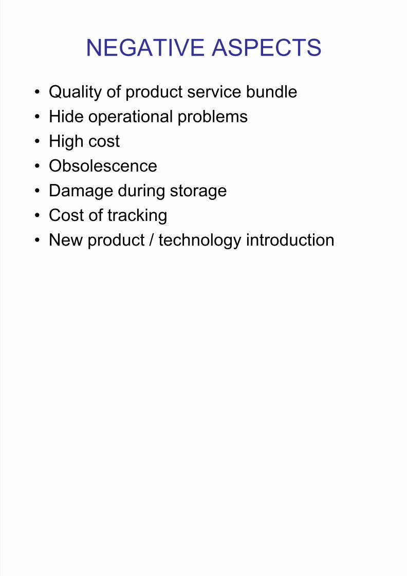
NEGATIVE ASPECTS
Quality of product service bundle
Hide operational problems
High cost Obsolescence
Damage during storage
Cost of tracking New product / technology introduction

8/3/2019 3445 Inventory Management
http://slidepdf.com/reader/full/3445-inventory-management 5/44
STOCK POINTS
SUPPLIERS DISTRIBUTOR RETAILER
RM, RM, INPROCESS INV PRODUCT PRODUCT
COMPONENTS COMPONENTS PIPELINE INV
VALUE ADDING S YSTEM
FINISHED GOODS

8/3/2019 3445 Inventory Management
http://slidepdf.com/reader/full/3445-inventory-management 6/44
E(1
)
Independent vs. Dependent
Demand
Independent Demand (Demand for the final end-
product or demand not related to other items)
Dependent
Demand
(Derived demand
items for component
parts,
subassemblies,
raw materials,
etc)
Finished
product
Component parts

8/3/2019 3445 Inventory Management
http://slidepdf.com/reader/full/3445-inventory-management 7/44
Inventory Systems
Single-Period Inventory Model
± One time purchasing decision (Example:
vendor selling t-shirts at a cricket game)
± Seeks to balance the costs of inventory
overstock and under stock
Multi-Period Inventory Models
± Fixed-Order Quantity Models
Event triggered (Example: running out of
stock)
± Fixed-Time Period Models
Time triggered (Example: Monthly sales call
by sales representative)

8/3/2019 3445 Inventory Management
http://slidepdf.com/reader/full/3445-inventory-management 8/44
INVENTORY CONTROL SYSTEM
When to order
How much to order
Buffer Stock
Maximum Inventory
How often to review stock

8/3/2019 3445 Inventory Management
http://slidepdf.com/reader/full/3445-inventory-management 9/44
COSTS
Holding (or carrying) costs
± Costs for storage, handling, insurance, etc
Setup (or production change) costs
± Costs for arranging specific equipment
setups, etc
Ordering costs
± Costs of someone placing an order,transportation etc
Shortage costs

8/3/2019 3445 Inventory Management
http://slidepdf.com/reader/full/3445-inventory-management 10/44
SINGLE PERIOD
d + z *

8/3/2019 3445 Inventory Management
http://slidepdf.com/reader/full/3445-inventory-management 11/44
Single-Period Inventory Model
uo
u
C C
C P
e
sold beunit willy that theProbabilit
estimatedunder demandof unit per CostCestimatedover demandof unit per CostC
:Where
u
o
!
!
!
P

8/3/2019 3445 Inventory Management
http://slidepdf.com/reader/full/3445-inventory-management 12/44
Single Period Model Example
Our college basketball team is playing in atournament game this weekend. Based on our
past experience we sell on average 2,400 shirtswith a standard deviation of 350. We makeRs100 on every shirt we sell at the game, but loseRs50 on every shirt not sold. How many shirtsshould we make for the game?
C u = Rs100 and C o = Rs50; P 100 / (100 + 50) = .667
Z.667 = .432 (use NORMSINV(.667))
therefore we need 2,400 + .432(350) = 2,551 shirts

8/3/2019 3445 Inventory Management
http://slidepdf.com/reader/full/3445-inventory-management 13/44
UNCERTAIN DEMAND
UNIT COST = 1
SALE PRICE = 2
PURCHASE 30
DEMAND PROB SOLD EARN COST PROFIT
profit10 0.05 10 20 30 -10 -0.5
20 0.15 20 40 30 10 1.5
30 0.3 30 60 30 30 9
40 0.2 30 60 30 30 6
50 0.1 30 60 30 30 3
60 0.1 30 60 30 30 3
70 0.1 30 60 30 30 3
Probable profit 25

8/3/2019 3445 Inventory Management
http://slidepdf.com/reader/full/3445-inventory-management 14/44
UNCERTAIN DEMAND
UNIT COST = 1
SALE PRICE = 2
PURCHASE 30
DEMAND PROB SOLD EARN COST PROFITO
PORT
UNITY
LOST
Probableprofit
10 0.05 10 20 30 -10 0 -0.5
20 0.15 20 40 30 10 0 1.5
30 0.3 30 60 30 30 0 9
40 0.2 30 60 30 30 -10 4
50 0.1 30 60 30 30 -20 1
60 0.1 30 60 30 30 -30 0
70 0.1 30 60 30 30 -40 -1
Probable profit 14

8/3/2019 3445 Inventory Management
http://slidepdf.com/reader/full/3445-inventory-management 15/44
Fixed-Order Quantity Model
Assumptions Demand for the product is constant
and uniform throughout the period
Lead time (time from ordering toreceipt) is constant
Price per unit of product is constant
Instantaneous replacement

8/3/2019 3445 Inventory Management
http://slidepdf.com/reader/full/3445-inventory-management 16/44
FIXED ORDER QU ANTITY
QTY
TIME
ORDER
QU ANTITY
AVERAGE
INVENTORY
REORDER
POINT

8/3/2019 3445 Inventory Management
http://slidepdf.com/reader/full/3445-inventory-management 17/44
Fixed-Order Quantity Model Assumptions
Inventory holding cost is based onaverage inventory
Ordering or setup costs are constant
All demands for the product will be
satisfied (No back orders are allowed)

8/3/2019 3445 Inventory Management
http://slidepdf.com/reader/full/3445-inventory-management 18/44
TOTAL COST
H2Q +S
QD +DC=TC
Total Annual =Cost
AnnualPurchase
Cost
AnnualOrdering
Cost
AnnualHolding
Cost+ +

8/3/2019 3445 Inventory Management
http://slidepdf.com/reader/full/3445-inventory-management 19/44
Q = 2DSH
= 2(Annual Demand)(Order or Setup Cost)Annual Holding CostOPT
EOQ

8/3/2019 3445 Inventory Management
http://slidepdf.com/reader/full/3445-inventory-management 20/44
Cost Minimization
Ordering Costs
Holding
Costs
Order Quantity (Q)
COST
Annual Cost of
Items (DC)
Total Cost
QOPT

8/3/2019 3445 Inventory Management
http://slidepdf.com/reader/full/3445-inventory-management 21/44
REORDER POINT
Reorder point, R = d L _
d = average daily demand (constant)
L = Lead time (constant)
_

8/3/2019 3445 Inventory Management
http://slidepdf.com/reader/full/3445-inventory-management 22/44
EOQ Example
Annual Demand = 1,000 unitsCost to place an order = Rs10
Holding cost per unit per year = Rs2.50
Lead time = 7 days
Cost per unit = Rs15
Given the information below, what are the EOQ and
reorder point?
Q =((2*1000*10)/2.5)^1/2 = 4000
ROP= (1000/250)*7 = 28

8/3/2019 3445 Inventory Management
http://slidepdf.com/reader/full/3445-inventory-management 23/44
PRICE DISCOUNT
0
5000
10000
15000
20000
25000
30000
35000
40000
45000
50000
1 2 3 4 5 6 7 8 9 10 11 12 13 14 15 16 17 18 19 20
OQ
CO
IC
PC
TC

8/3/2019 3445 Inventory Management
http://slidepdf.com/reader/full/3445-inventory-management 24/44
Price-Break Example Problem
A company has a chance to reduce their costs by
placing larger quantity orders using the price-break
order quantity schedule below. What should their
optimal order quantity be if this company purchases
this single inventory item with an ordering cost of
Rs4, a carrying cost rate of 2% of the inventory cost
of the item, and an annual demand of 10,000 units?
Order Quantity(units) Price/unit(Rs)0 to 2,499 Rs1.202,500 to 3,999 1.004,000 or more .98

8/3/2019 3445 Inventory Management
http://slidepdf.com/reader/full/3445-inventory-management 25/44
Price-Break
units1,826=0.02(1.20)
4)2(10,000)( =
iC
2DS =QOPT
Annual Demand (D)= 10,000 unitsCost to place an order (S)= Rs4
First, plug data into formula for each price-break value of ³C´
units2,000=0.02(1.00)
4)2(10,000)( =
iC
2DS =QOPT
units2,020=0.02(0.98)
4)2(10,000)( =
iC
2DS =QOPT
Carrying cost % of total cost (i)= 2%Cost per unit (C) = $1.20, $1.00, $0.98
Interval from 0 to 2499, theQopt value is feasible
Interval from 2500-3999, theQopt value is not feasible
Interval from 4000 & more, theQopt value is not feasible
Next, determine if the computed Qopt values are feasible or not

8/3/2019 3445 Inventory Management
http://slidepdf.com/reader/full/3445-inventory-management 26/44
Price-Break
Since the feasible solution occurred in the first price-break, it means that all the other true Qopt values occur
at the beginnings of each price-break interval. Why?
0 1826 2500 4000 Order Quantity
Totalannualcosts So the candidates
for the price-
breaks are 1826,2500, and 4000
units
Because the total annual cost function isa ³u´ shaped function

8/3/2019 3445 Inventory Management
http://slidepdf.com/reader/full/3445-inventory-management 27/44
Price-Break
iC2
Q +S
Q
D +DC=TC
TC(0-2499)=(10000*1.20)+(10000/1826)*4+(1826/2)(0.02*1.20)
= Rs12,043.82TC(2500-3999)= Rs10,041
TC(4000&more)= Rs9,949.20
8/3/2019 3445 Inventory Management
http://slidepdf.com/reader/full/3445-inventory-management 28/44
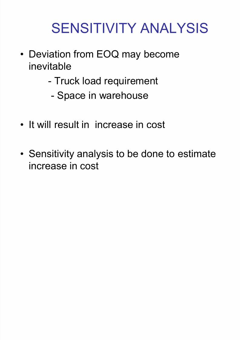
SENSITIVITY ANALYSIS
Deviation from EOQ may becomeinevitable
- Truck load requirement- Space in warehouse
It will result in increase in cost
Sensitivity analysis to be done to estimate
increase in cost

8/3/2019 3445 Inventory Management
http://slidepdf.com/reader/full/3445-inventory-management 29/44
VARIABLE LEAD TIME ,DEMAND
QTY
TIME
SAFETY
STOCK
REORDER
POINT
ORDER
QU ANTITY

8/3/2019 3445 Inventory Management
http://slidepdf.com/reader/full/3445-inventory-management 30/44
SAFETY STOCK
Safety Stock - Stock that is held inexcess of expected demand due tovariable demand rate and/or lead time.
Service Level - Probability that demandwill not exceed supply during lead time.

8/3/2019 3445 Inventory Management
http://slidepdf.com/reader/full/3445-inventory-management 31/44
OP for Discrete DDLT
DistributionOne of Sharp Retailer¶s inventory items isnow being analyzed to determine anappropriate level of safety stock. The
manager wants an 80% service level duringlead time. The item¶s historical DDLT is:
DDLT (units) Occurrences3 8
4 65 46 2

8/3/2019 3445 Inventory Management
http://slidepdf.com/reader/full/3445-inventory-management 32/44
OP for Discrete DDLT
Distribution
Probability Probability of
DDLT (cases) of DDLT DDLT or Less
3 .4 .44 .3 .75 .2 .9
6 .1 1.0To provide 80% service level, OP = 5
cases

8/3/2019 3445 Inventory Management
http://slidepdf.com/reader/full/3445-inventory-management 33/44
REORDER POINT
ROP
Risk of a stockout
Service level
Probability of
no stockout
Expected
demand Safety
stock
0 z
Quantity
z-scale
The ROP based on a normalDistribution of lead time demand

8/3/2019 3445 Inventory Management
http://slidepdf.com/reader/full/3445-inventory-management 34/44
SAFETY STOCKVARIABLE DEMAND
Average demand during lead time
Standard deviation of Demand During lead
time

8/3/2019 3445 Inventory Management
http://slidepdf.com/reader/full/3445-inventory-management 35/44
SAFETY STOCKVARIABLE DEMAND
ROP = Average demand during lead time + z * standard deviation of demand during lead time
-
ROP = d + z * sd( demand during lead time)
sd (demand during lead time ) =
8/3/2019 3445 Inventory Management
http://slidepdf.com/reader/full/3445-inventory-management 36/44
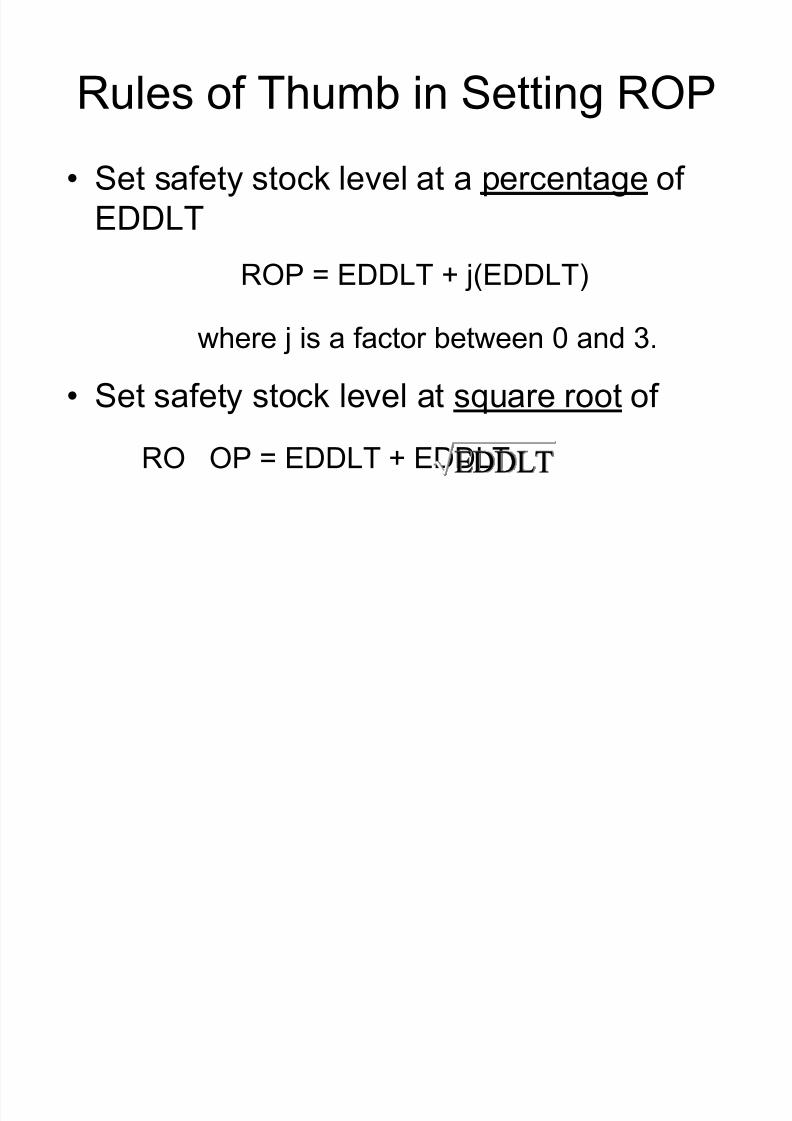
Set safety stock level at a percentage of EDDLT
ROP = EDDLT + j(EDDLT)
where j is a factor between 0 and 3.
Set safety stock level at square root of
RO OP = EDDLT + EDDLT
Rules of Thumb in Setting ROP
EDDLT

8/3/2019 3445 Inventory Management
http://slidepdf.com/reader/full/3445-inventory-management 37/44
FIXED PERIOD MODEL
L L T L
T T

8/3/2019 3445 Inventory Management
http://slidepdf.com/reader/full/3445-inventory-management 38/44
FIXED REORDER CYCLE
D = demand for the year
T = Time between orders ( fraction of year)
Average inventory = D*T/2
Orders per year = 1/T
Total Inv Cost = CO * (1/T) +(D*T/2) * IC
8/3/2019 3445 Inventory Management
http://slidepdf.com/reader/full/3445-inventory-management 39/44
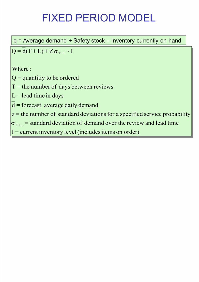
order )onitems(includeslevelinventorycurrent=I
timeleadandreviewover thedemandof deviationstandard=
y probabilitservicespecifiedafor deviationsstandardof number the=zdemanddailyaverageforecast=d
daysintimelead=L
reviews betweendaysof number the=T
ordered betoquantitiy=Q:Where
I-Z+L)+(Td=Q
L+T
L+T
W
W
q = Average demand + Safety stock ± Inventory currently on hand
FIXED PERIOD MODEL

8/3/2019 3445 Inventory Management
http://slidepdf.com/reader/full/3445-inventory-management 40/44
Maximum Inventory Level, M
Optional Replenishment System
MActual Inventory Level, I
q = M - I
I
Q = minimum acceptable order quantity
If q > Q, order q, otherwise do not order any.

8/3/2019 3445 Inventory Management
http://slidepdf.com/reader/full/3445-inventory-management 41/44
ABC Classification System
Items kept in inventory are not of equalimportance in terms of:
± Rupees invested
± profit potential
± sales or usage volume
± stock-out penalties
0
30
60
30
60
AB
C
% of
Rs Value
% of Use
So, identify inventory items based on percentage of total
consumption, where ³A´ items are roughly top 80 %, ³B´
items as next 15 %, and the lower 5% are the ³C´ items

8/3/2019 3445 Inventory Management
http://slidepdf.com/reader/full/3445-inventory-management 42/44
Inventory Accuracy and Cycle Counting
Inventory accuracy refers to how
well the inventory records agreewith physical count
Cycle Counting is a physical
inventory-taking technique in whichinventory is counted on a frequent
basis rather than once or twice a
year

8/3/2019 3445 Inventory Management
http://slidepdf.com/reader/full/3445-inventory-management 43/44
Inventory Counting Systems
P eriodic System
Physical count of items made at periodicintervals
P erpetual Inventory SystemSystem that keeps trackof removals from inventorycontinuously, thus
monitoringcurrent levels of each item

8/3/2019 3445 Inventory Management
http://slidepdf.com/reader/full/3445-inventory-management 44/44
Inventory Counting Systems
Tw o-Bin System - Two containers of inventory; reorder when the first is empty
Universal Bar Code - Bar code
printed on a label that hasinformation about the itemto which it is attached
0
214800 232087768