328-2012: Introducing the FMM Procedure for Finite … the FMM Procedure for Finite Mixture Models...

Paper 328-2012

Introducing the FMM Procedure for Finite Mixture ModelsDave Kessler and Allen McDowell, SAS Institute Inc., Cary, NC

ABSTRACT

You’ve collected the data and performed a preliminary analysis with a linear regression. But the residuals have sev-eral modes, and transformations don’t help. You need a different approach, and that calls for the FMM procedure.PROC FMM fits finite mixture models, which enable you to describe your data with mixtures of different distributionsso you can account for underlying heterogeneity and address overdispersion. PROC FMM offers a wide selectionof continuous and discrete distributions, and it provides automated model selection to help you choose the numberof components. Bayesian techniques are also available for many analyses. This paper provides an overview of thecapabilities of the FMM procedure and illustrates them with applications drawn from a variety of fields.

INTRODUCTION

Most statistical methods assume that you have a sample of observations, all of which come from the same distribution,and that you are interested in modeling that one distribution. If you actually have data from more than one distributionwith no information to identify which observation goes with which distribution, standard models won’t help you. However,finite mixture models might come to the rescue. They use a mixture of parametric distributions to model data, estimatingboth the parameters for the separate distributions and the probabilities of component membership for each observation.

Finite mixture models provide a flexible framework for analyzing a variety of data. Suppose your objective is to describethe distribution of a response variable. If the corresponding data are multimodal, skewed, heavy-tailed, or exhibitkurtosis, they may not be representative of most known distributions. In this case, you often use a nonparametricmethod such as kernel density estimation to describe the distribution. A kernel density estimate generates a smoothed,numerical approximation to the unknown distribution function and estimates the distribution’s percentiles. Although thisapproach is useful, it might not be the most concise way to describe an unknown distribution. A finite mixture modelprovides a parametric alternative that describes the unknown distribution in terms of mixtures of known distributions.A finite mixture model also enables you to assess the probabilities of events or simulate draws from the unknowndistribution the same way you do when your data are from a known distribution.

Finite mixture models also provide a parametric modeling approach to one-dimensional cluster analysis. This approachuses the fitted component distributions and the estimated mixing probabilities to compute a posterior probability of com-ponent membership. An observation is assigned membership to the component with the maximum posterior probability.A benefit of using a model-based approach to clustering is that it permits estimation and hypothesis testing within theframework of standard statistical theory (McLachlan and Basford 1988).

Finally, finite mixture models provide a mechanism that can account for unobserved heterogeneity in the data. Certainimportant classifications of the data (such as region, age group, or gender) are not always measured. These latent clas-sification variables can introduce underdispersion, overdispersion, or heteroscedasticity in a traditional model. Finitemixture models overcome these problems through their more flexible form.

FINITE MIXTURE MODELS

Consider a data set that is composed of people’s body weights. Figure 1 presents the pooled data. The histogramindicates an asymmetric distribution with three modes. Figure 2 displays separate histograms for age group andgender. Each distribution is symmetric, with only one mode.

1

Statistics and Data AnalysisSAS Global Forum 2012

Figure 1 Pooled Body Weights Figure 2 Body Weights Classified by Age and Gender

The histograms in Figure 2 explain the structure in Figure 1. This illustrates a problem that arises in many situations:you might not know important predictors for the response. Without this information, models fit by using traditionaltechniques can perform poorly. The finite mixture model can account for these unknown predictors.

The previous example demonstrates how a mixture can arise when you do not observe important predictors. In othersituations, you might have all of the important predictors, but the response does not follow a well-known distribution. Thehistogram in Figure 3 demonstrates a case where the response distribution has a strong central mass and heavy tails.A single Gaussian or t distribution would not provide a satisfactory model for these data. However, you could modelthis response with a mixture of one low-variance Gaussian distribution and another high-variance Gaussian distribution,each with the same mean. Figure 3 displays these separate component densities and the weighted combination thatforms the mixture model. In this case, the finite mixture model provides a more flexible form for the response distribution.

Figure 3 Distribution with Unusual Structure

The expression for the density or likelihood of a response value y in a general k-component finite mixture model is:

f .y/ D

kXjD1

�j .z;˛j /pj .yIx0j ˇj ; �j /

In this model, the parametric distributions pj are weighted by the mixing probabilities �j . The component distributionspj can depend on regressor variables in xj , regression parameters ˇj , and possibly scale parameters �j . The mixingprobabilities �j , which sum to 1, can depend on regressor variables z and corresponding parameters ˛j . Theseprobabilities can be modeled using a logit transform if k D 2, and as a generalized logit model if k > 2. The componentdistributions pj are indexed by j because the distributions might belong to different families. For example, to manageoverdispersion in a two-component model, you might model one component as a normal (Gaussian) variable and thesecond component as a variable with a t distribution with low degrees of freedom.

2


BASIC FEATURES OF THE FMM PROCEDURE

The FMM procedure, experimental in SAS/STAT® 9.3, fits finite mixture models to univariate outcomes by both max-imum likelihood and Bayesian techniques. PROC FMM fits finite mixtures of linear regression models or generalizedlinear models, and it models both the component distributions and the mixing probabilities. The procedure’s model-building syntax includes the CLASS and MODEL statements that are familiar from other SAS/STAT procedures suchas the GLM, GLIMMIX, and MIXED procedures. PROC FMM features a BAYES statement for specifying a Bayesiananalysis, as do the GENMOD, LIFEREG, and PHREG procedures.

In addition, PROC FMM provides the following features:

� many built-in link and distribution functions for modeling, including the beta, shifted t , Weibull, beta-binomial, andgeneralized Poisson distributions, in addition to many standard members of the exponential family of distributions

� specialized built-in mixture models such as the binomial cluster model and the ability to add zero-inflation to anymodel

� ability to build mixture models in which the model effects, distributions, or link functions vary across mixturecomponents by using multiple MODEL statements

� evaluation of sequences of mixture models when you specify ranges for the number of components

� simple syntax to impose linear equality and inequality constraints among parameters

� ability to model regression and classification effects in the mixing probabilities by using the PROBMODEL state-ment

� ability to incorporate fully or partially known component membership into the analysis

� ability to produce a SAS data set with important statistics for interpreting mixture models, such as component loglikelihoods and prior and posterior probabilities by using the OUTPUT statement

� output data set with posterior parameter values for the Markov chain

� high degree of multithreading for high-performance optimization and Monte Carlo sampling

ESTIMATION METHODS

The FMM procedure provides maximum likelihood estimation for numerous continuous and discrete response distribu-tions. It uses a dual quasi-Newton optimization algorithm by default, but you can choose from several other optimizationtechniques to produce the maximum likelihood estimates.

Bayesian analysis is supported for a smaller set of response distributions. For these distributions, PROC FMM pro-vides a single parametric form for the prior distributions, but you can adjust the prior parameters to reflect specificprior information. The Bayesian methods in PROC FMM use a data augmentation scheme for improved MCMC per-formance. Gibbs sampling is used by default; but when this is not possible, PROC FMM uses a Metropolis-Hastingsalgorithm originally proposed by Gamerman (1997). Both methods produce a posterior sample that provides the basisfor inference.

Example 1: Accounting for Excess Zeros

This example applies several alternative mixture models to illustrate the use of PROC FMM where a mixture distributionprovides improvement over a standard Poisson regression for count data.

Greene (1995) presents data for a set of 1,319 individuals drawn at random from the applicant pool for a credit card. Amajor derogatory report (MDR) is an event such as a foreclosure, a collection action, or an account that is delinquentfor 120 days or more. The researchers were interested in modeling MDR counts as a function of other variables—inparticular, the age of the applicant (Age), their income in units of $10,000 (Income), their average monthly credit cardexpenditure (Avgexp), and their homeowner status (Ownrent).

The first step in an analysis is to look at the data graphically. The following DATA step creates the data set CREDRPT,and the SGPLOT procedure creates a histogram that provides an overall impression of the distribution of MDR counts.

data credrpt;input MDR Age Income Avgexp Ownrent;datalines;

0 37.6667 4.5200 124.9833 1

3


0 33.2500 2.4200 9.8542 00 33.6667 4.5000 15.0000 10 30.5000 2.5400 137.8692 00 32.1667 9.7867 546.5033 10 23.2500 2.5000 91.9967 0

... more lines ...

0 40.5833 4.6000 101.2983 10 32.8333 3.7000 26.9967 00 48.2500 3.7000 344.1575 1;run;

proc sgplot data=credrpt;histogram mdr / showbins;

run;

Figure 4 presents the resulting histogram; 80.4% of the applicants had no MDRs.

Figure 4 Histogram of MDR Counts

You might decide to perform a Poisson regression that models MDR count as a function of the applicant’s age, income,and average monthly credit card spending. Poisson regression is a standard technique for analyzing count data; itassumes that the mean and the variance are equal. The GENMOD procedure is the standard SAS/STAT tool forperforming Poisson regression, but you can fit a Poisson regression with PROC FMM too as a mixture model with justone component. You specify the model in PROC FMM the same way as you would in PROC GENMOD; the log linkis applied by default with the DIST=POISSON option. The following SAS statements produce the Poisson regressionanalysis:

proc fmm data=credrpt;model mdr = age income avgexp / dist=poisson;

run;

Output 1 summarizes information about this model and its fit statistics.

Output 1 Poisson Model

Poisson Model

The FMM Procedure

Model Information

Data Set WORK.CREDRPTResponse Variable MDRType of Model Generalized Linear (GLM)Distribution PoissonComponents 1Link Function LogEstimation Method Maximum Likelihood

4


Output 1 continued

Number of Observations Read 1319Number of Observations Used 1319

Fit Statistics

-2 Log Likelihood 2793.4AIC (smaller is better) 2801.4AICC (smaller is better) 2801.5BIC (smaller is better) 2822.2Pearson Statistic 9362.5

The value of the Pearson statistic is 9362.5. Its value should approach the sample size of 1,319 if the underlyingassumptions are satisfied. The large value of 9362.5 indicates that the model fit is questionable, and it suggests thatthe variance exceeds the mean. When this happens, the model is said to exhibit overdispersion. So the Poisson modeldoes not appear to describe these data well.

Consider Figure 4 again. Another way to view these data is as a mixture of a constant distribution (which alwaysgenerates zero counts) and a truncated Poisson distribution (which always generates nonzero counts). The mixingprobabilities estimate the corresponding probabilities that an observation is drawn from one of the two distributions.This is called a hurdle model (Mullahy 1986).

You fit a hurdle model in PROC FMM by using two MODEL statements. One MODEL statement specifies a truncatedPoisson distribution for the nonzero MDR group. The other MODEL statement specifies a constant distribution with allmass at zero for the zero MDR group. The truncated Poisson MODEL statement includes covariates, but the MODELstatement for the constant distribution does not. Finally, you can make the mixing probabilities themselves depend onthe covariates by including them in the PROBMODEL statement.

proc fmm data=credrpt;model mdr = age income avgexp / dist=tpoisson;model mdr = / dist=constant;probmodel age income ownrent;

run;

Output 2 displays the model information and fit statistics for the Poisson hurdle model. The Pearson statistic of 1747.7indicates a better fit than the original Poisson regression model.

Output 2 Poisson Hurdle Model

Poisson Hurdle Model

The FMM Procedure

Model Information

Data Set WORK.CREDRPTResponse Variable MDRType of Model Poisson HurdleComponents 2Estimation Method Maximum Likelihood

Fit Statistics

-2 Log Likelihood 2177.1AIC (smaller is better) 2193.1AICC (smaller is better) 2193.2BIC (smaller is better) 2234.6Pearson Statistic 1747.7Effective Parameters 8Effective Components 2

The concept of the hurdle model is that the data are separated into one group of people who will have at least oneMDR and another group of people who will have no MDRs. But it might be more reasonable to model the groups aspeople who might have a MDR and people who will never have an MDR. In other words, people in the first group areat risk for a MDR but might not experience one, and people in the second group are at no risk for a MDR and willnever experience one. You can address this scenario with the zero-inflated Poisson (ZIP) model (Lambert 1992). TheZIP model uses a Poisson distribution in place of the truncated Poisson distribution used by the hurdle model. So,while the hurdle model restricts the zeros to one component, the ZIP model permits the zero counts to come from bothcomponents in the model.

5


You fit the ZIP model by specifying DIST=POISSON in the first MODEL statement; the rest of the PROC FMM state-ments remain the same:

proc fmm data=credrpt gconv=0;model mdr = age income avgexp / dist=poisson;model mdr = / dist=constant;probmodel age income ownrent;

run;

Output 3 presents the model information and the fit statistics for the ZIP model. The Pearson statistic has the value2026.4, which is better than the value for the standard Poisson model but worse than the value for the hurdle model.

Output 3 Zero-Inflated Poisson Model

Zero-Inflated Poisson Model

The FMM Procedure

Model Information

Data Set WORK.CREDRPTResponse Variable MDRType of Model Zero-inflated PoissonComponents 2Estimation Method Maximum Likelihood

Fit Statistics


Another alternative is the zero-inflated negative binomial (ZINB) model. The ZINB model permits zero counts to comefrom both component distributions (similar to the ZIP model), but it uses a negative binomial distribution instead of aPoisson distribution. The following statements specify the ZINB model; the DIST=NEGBIN option in the first MODELstatement requests the negative binomial distribution:

proc fmm data=credrpt;model mdr = age income avgexp / dist=negbin;model mdr = / dist=constant;probmodel age income ownrent;

run;

Output 4 displays the fit statistics for the new model. The Pearson statistic is 1355.3, which indicates the best fit of allthe models.

Output 4 Zero-Inflated Negative Binomial Model

Zero-Inflated Negative Binomial

The FMM Procedure

Model Information

Data Set WORK.CREDRPTResponse Variable MDRType of Model Zero-inflated NegBinomialComponents 2Estimation Method Maximum Likelihood

Fit Statistics


6


Output 5 presents the estimates for both the negative binomial component parameters and the mixing probability modelparameters. You can refine this model by removing variables that are not significant from the model for MDR counts orfrom the model for the mixing probabilities.

Output 5 Zero-Inflated Negative Binomial Parameter Estimates

Parameter Estimates for 'Negative Binomial' Model

StandardComponent Effect Estimate Error z Value Pr > |z|

1 Intercept 0.2543 0.4712 0.54 0.58951 Age -0.01394 0.01013 -1.38 0.16901 Income 0.02749 0.05296 0.52 0.60371 Avgexp -0.00200 0.000366 -5.47 <.00011 Scale Parameter 2.9799 0.6853

Parameter Estimates for Mixing Probabilities

StandardEffect Estimate Error z Value Pr > |z|

Intercept -3.3052 1.0452 -3.16 0.0016Age 0.1125 0.04316 2.61 0.0092Income 0.2611 0.1708 1.53 0.1264Ownrent -0.8853 0.3890 -2.28 0.0229

Table 1 compares the information criteria for all four models and provides relative rankings for the models by eachcriterion. All of the information criteria tell the same story for these data: the ZINB model ranks first by all five criteria,followed by the Poisson hurdle model, the ZIP model, and the standard Poisson model.

Table 1 Information Criteria Comparisons with Relative Rankings

Model –2LL AIC AICC BIC Pearson

Poisson 2793.4 (4) 2801.4 (4) 2801.5 (4) 2822.2 (4) 9362.5 (4)Poisson hurdle 2177.1 (2) 2193.1 (2) 2193.2 (2) 2234.6 (2) 1747.7 (2)ZIP 2186.1 (3) 2202.1 (3) 2202.2 (3) 2243.5 (3) 2026.4 (3)ZINB 2053.5 (1) 2071.5 (1) 2071.6 (1) 2118.2 (1) 1355.3 (1)

You can also assess the performance of the different models by computing the predicted probability of different MDRcounts for each observation, averaging those probabilities, and comparing the results to the observed relative frequen-cies of MDR counts (Long 1997).

Figure 5 displays the difference between the computed MDR count frequencies for each model and the observedrelative frequencies (the SAS statements are not shown).

Figure 5 Model Comparison

7


The ZINB model appears to fit the data best, and the Poisson hurdle model is a close second. The standard Poissonmodel performed poorly for the most frequent counts. It appears that a split-population model like the hurdle, ZIP, orZINB model is useful for describing these data. However, a split of the population into different groups is not necessarilythe true state of nature; the MDR counts might follow a zero-heavy model unlike any you know. A finite mixturemodeling approach enables you to take simple, well-understood models and combine them in a way that provides abetter description of the data than a single-component model provides.

Example 2: Clustering of Rare Events

The FMM procedure also enables you to use a parametric model to perform clustering for univariate data. The finitemixture model approach to clustering assumes that the observations to be clustered are drawn from a mixture of aspecified number of groups in varying proportions. A distribution is chosen for each group; the distributions can be, butare not required to be, the same for all of the groups. You fit the finite mixture model to estimate the model parametersand the posterior probabilities of group membership. Each observation is then assigned membership to the group forwhich it has the highest estimated posterior probability of belonging (McLachlan and Basford 1988).

For example, Symons, Grimson, and Yuan (1983) used a finite mixture model to study the incidence of sudden infantdeath syndrome (SIDS) in North Carolina; they focus on identifying counties at high risk for SIDS. Table 2 describesthe variables used in the analysis.

Table 2 NCSIDS Data Set

Variable Name Description

County Name of countyBirths Number of recorded live births (1974–1978)SIDS Number of recorded SIDS cases (1974–1978)Rate Incidence rate (SIDS/Births)Logrisk Natural logarithm of the size of the at-risk population

An initial approach to analyzing these data for the presence of clusters is to examine a plot of the ordered SIDSincidence rates. Gaps in the ordered rates might indicate the presence of separate risk groups in the overall population.

The following SAS statements read the data and create the data set NCSIDS. PROC RANK ranks the rates in descend-ing order and stores the result in the variable Order. The SGPLOT procedure produces a scatter plot of Rate versusOrder and a scatter plot of Rate versus Births.

data ncsids;input County $ 1-12 Births SIDS;Rate=SIDS/Births;Logrisk=log(Births);datalines;

Alamance 4672 13Alexander 1333 0Alleghany 487 0Anson 1570 15Ashe 1091 1Avery 781 0Beaufort 2692 7

... more lines ...

Wilson 3702 11Yadkin 1269 1Yancey 770 0;

proc rank data=ncsids out=ncsids descending;var rate;ranks order;

run;

proc sgplot data=ncsids;scatter x=order y=rate / markerattrs=(symbol=CircleFilled size=4px);refline 0.0029 0.0035 / axis=y lineattrs=(pattern=dot);

run;

8


proc sgplot data=ncsids;scatter x=Births y=rate /markerattrs=(symbol=CircleFilled size=4px) ;yaxis values=(.001 .002 .003 .004 .005 .006 .007 .008 .009 .01);refline 0.0029 0.0035 / axis=y lineattrs=(pattern=dot);

run;

Figure 6 displays the plot of the ordered incidence rates. There appears to be a gap in the rates around 0.0029–0.0035.However, Figure 7 shows that the higher SIDS rates appear to be concentrated in counties with a lower number of births.This means that the higher rates tend to be measured with low precision. So, classifying the counties based solely ona visual inspection of ordered rate magnitudes can be misleading because the rates are not measured with the sameprecision. Fitting a finite mixture model enables you to estimate group membership by taking into account both themagnitude and the precision of the estimated rates.

Figure 6 Ordered Incidence Rates Figure 7 SIDS Incidence Rates by Births

Following Symons, Grimson, and Yuan (1983), assume that the counties are a mixture of a normal-risk group and ahigh-risk group and that the number of SIDS cases follows different Poisson distributions for each group. When you usePROC FMM to fit this model, the procedure computes the posterior probabilities of component membership for eachobservation as

P r.j jyi / D�jpj .yI�j /Pk

jD1 �jpj .yI�j /

where �j is the mixing probability (prior probability) for the j th component and �j is the mean for the j th component.Each observation is then allocated to either the high-risk or normal-risk group according to which group has the largestposterior probability.

The following SAS statements perform the analysis. By default, PROC FMM uses a log link function when you specifyDIST=POISSON. The KMAX=2 option requests that one- and two- component models be fitted and considered forselection. The CLASS option in the OUTPUT statement generates a variable named ML in the output data set thatcontains the model-based group allocations for each observation.

proc fmm data=ncsids;model SIDS = / dist=poisson kmax=2 offset=Logrisk;output out=Max class=ML;

run;

Output 6 presents the details of the model selection; all but one of the criteria favor the two-component model. Bydefault, PROC FMM uses the –2*log-likelihood criteria for model selection, but you can use the CRITERION= option inthe PROC FMM statement to specify an alternative.

9


Output 6 Evaluation of One- and Two-Component Models for SIDS Data

The FMM Procedure

Component Evaluation for Mixture Models

-------- Number of -------Model -Components- -Parameters- Max

ID Total Eff. Total Eff. -2 Log L AIC AICC BIC Pearson Gradient

1 1 1 1 1 508.75 510.75 510.79 513.36 225.57 1.655E-62 2 2 3 3 474.27 480.27 480.52 488.09 113.25 0.000090

The model with 2 components (ID=2) was selected as 'best' based on the -2 log-likelihoodfunction.

Output 7 displays the parameter estimates for the two-component model. PROC FMM uses the logarithm of the ratesin its modeling, but it presents the parameter estimates on the original scale in the Inverse Linked Estimate column.The estimated component means are 0.001693 and 0.003805. The estimate of the mixing probability is 0.7969; this isthe weight for the first mixture component.

Output 7 Parameter Estimates for Two-Component Mixture

The FMM Procedure

Parameter Estimates for 'Poisson' Model

InverseStandard Linked

Component Parameter Estimate Error z Value Pr > |z| Estimate

1 Intercept -6.3813 0.08813 -72.41 <.0001 0.0016932 Intercept -5.5715 0.2289 -24.35 <.0001 0.003805


----------------Linked Scale---------------Standard

Parameter Estimate Error z Value Pr > |z| Probability

Probability 1.3668 0.8025 1.70 0.0885 0.7969

Output 8 lists the 19 counties with the highest SIDS incidence rates along with their group allocations. All of the othercounties are allocated to the normal-risk group.

Output 8 Frequentist Analysis

County SIDS Births Rate ML

Anson 15 1570 .00955 HighNorthampton 9 1421 .00633 HighWashington 5 990 .00505 HighHalifax 18 3608 .00499 HighHertford 7 1452 .00482 HighHoke 7 1494 .00469 HighGreene 4 870 .00460 HighBertie 6 1324 .00453 HighBladen 8 1782 .00449 HighColumbus 15 3350 .00448 HighSwain 3 675 .00444 NormalWarren 4 968 .00413 NormalRutherford 12 2992 .00401 HighRobeson 31 7889 .00393 HighLincoln 8 2216 .00361 HighRockingham 16 4449 .00360 HighScotland 8 2255 .00355 HighPender 4 1228 .00326 NormalWilson 11 3702 .00297 Normal

Figure 8 displays a scatter plot of the ordered incidence rates, and Figure 9 displays a scatter plot of the incidence ratesby the number of births. From this visual inspection, you might conclude that Swain and Warren counties, and possiblyPender and Wilson counties, are high-risk counties. However, these same counties are classified as normal-risk by

10


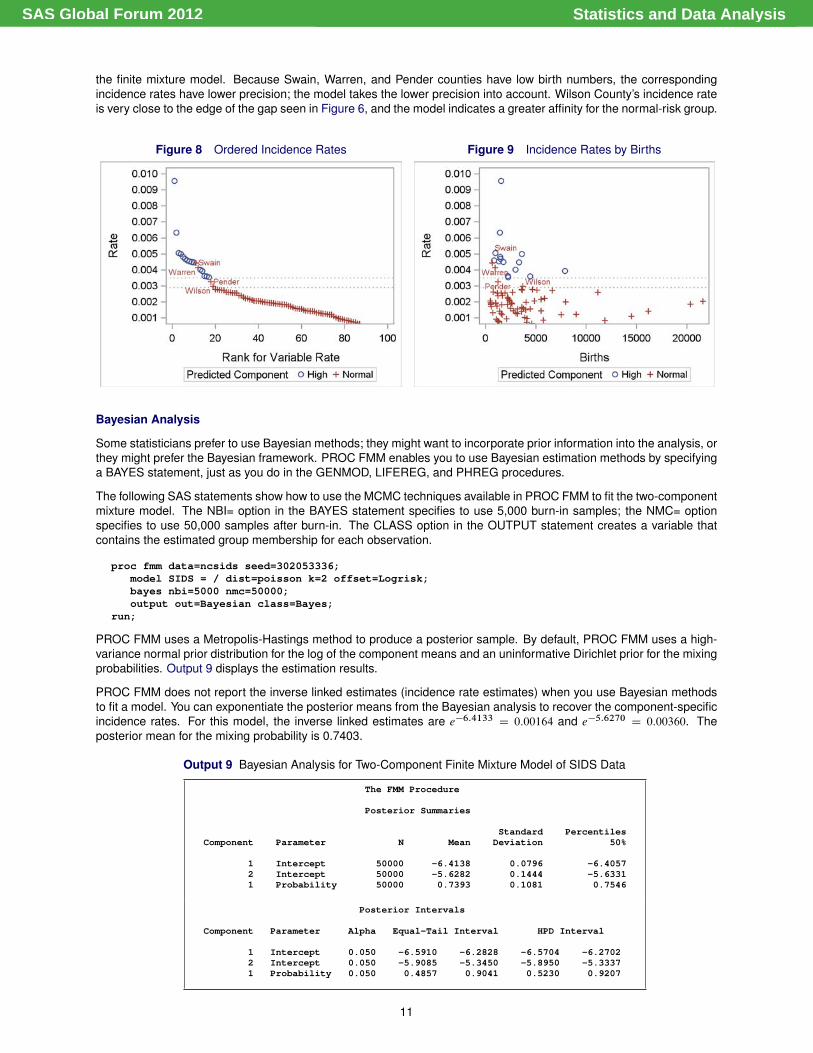
the finite mixture model. Because Swain, Warren, and Pender counties have low birth numbers, the correspondingincidence rates have lower precision; the model takes the lower precision into account. Wilson County’s incidence rateis very close to the edge of the gap seen in Figure 6, and the model indicates a greater affinity for the normal-risk group.

Figure 8 Ordered Incidence Rates Figure 9 Incidence Rates by Births

Bayesian Analysis

Some statisticians prefer to use Bayesian methods; they might want to incorporate prior information into the analysis, orthey might prefer the Bayesian framework. PROC FMM enables you to use Bayesian estimation methods by specifyinga BAYES statement, just as you do in the GENMOD, LIFEREG, and PHREG procedures.

The following SAS statements show how to use the MCMC techniques available in PROC FMM to fit the two-componentmixture model. The NBI= option in the BAYES statement specifies to use 5,000 burn-in samples; the NMC= optionspecifies to use 50,000 samples after burn-in. The CLASS option in the OUTPUT statement creates a variable thatcontains the estimated group membership for each observation.

proc fmm data=ncsids seed=302053336;model SIDS = / dist=poisson k=2 offset=Logrisk;bayes nbi=5000 nmc=50000;output out=Bayesian class=Bayes;

run;

PROC FMM uses a Metropolis-Hastings method to produce a posterior sample. By default, PROC FMM uses a high-variance normal prior distribution for the log of the component means and an uninformative Dirichlet prior for the mixingprobabilities. Output 9 displays the estimation results.

PROC FMM does not report the inverse linked estimates (incidence rate estimates) when you use Bayesian methodsto fit a model. You can exponentiate the posterior means from the Bayesian analysis to recover the component-specificincidence rates. For this model, the inverse linked estimates are e�6:4133 D 0:00164 and e�5:6270 D 0:00360. Theposterior mean for the mixing probability is 0.7403.

Output 9 Bayesian Analysis for Two-Component Finite Mixture Model of SIDS Data

The FMM Procedure

Posterior Summaries

Standard PercentilesComponent Parameter N Mean Deviation 50%

1 Intercept 50000 -6.4138 0.0796 -6.40572 Intercept 50000 -5.6282 0.1444 -5.63311 Probability 50000 0.7393 0.1081 0.7546

Posterior Intervals

Component Parameter Alpha Equal-Tail Interval HPD Interval

1 Intercept 0.050 -6.5910 -6.2828 -6.5704 -6.27022 Intercept 0.050 -5.9085 -5.3450 -5.8950 -5.33371 Probability 0.050 0.4857 0.9041 0.5230 0.9207

11


When you use the Bayesian techniques, you must check that the Markov chain that generates the posterior samplehas converged. This means that it really is a representative sample from the joint posterior distribution of the modelparameters. If it has converged, you can be comfortable about using the posterior sample for inference. If it has notconverged, any conclusions you draw will be suspect.

PROC FMM provides the same convergence diagnostics and plots as other SAS procedures that provide Bayesiananalysis. Output 10 displays the Markov Chain diagnostics plots for the first component. The trace plot at the topshows a relatively constant mean and variance for the posterior distribution, and the plot traverses the posterior spacefairly rapidly. These properties indicate that the chain has good mixing and is likely to be stationary, and that theburn-in sample is sufficiently large. The autocorrelation plot indicates that highly separated MCMC samples have lowcorrelation. Finally, the density plot shows a smooth and unimodal density function, indicating that the samples providea good representation of the posterior distribution.

Output 10 MCMC Diagnostic Plots

The Bayesian estimates of the component means and the mixing probability are different from those obtained by usingthe maximum likelihood method, so the estimates of the posterior probabilities, and thus some of the classifications,differ. Output 11 shows the counties where the classifications produced by the two estimation methods differ.

Output 11 Frequentist versus Bayesian Classification

County SIDS Births Rate ML Bayes

Warren 4 968 .004132231 Normal HighWilson 11 3702 .002971367 Normal HighAlamance 13 4672 .002782534 Normal HighWayne 18 6638 .002711660 Normal High

Figure 10 displays a scatter plot of the ordered incidence rates, and Figure 11 displays a scatter plot of the incidencerates by the number of births. The markers for the counties are coded according to the Bayesian classifications, and thefour counties whose Bayesian classifications differ from the frequentist classifications are labeled. The classificationsof Alamance and Wayne counties as high-risk are notable; they reflect the Bayesian model’s slightly smaller estimateof the high-risk group’s incidence rate.

12


Figure 10 Ordered Incidence Rates Figure 11 Incidence Rates by Births

Example 3: Complex Error Distributions

Linear regression is commonly used to model a variety of data. But when certain assumptions are not met, linearregression isn’t appropriate. For example, if important predictors for the response are unobserved, the parameterestimates will be inconsistent. If the residuals for the model do not follow the same distribution, the standard errors ofthe parameter estimates will be biased. This example demonstrates how finite mixture models can be used to modelsuch data.

Stukel (2008) provides a data set from an unpublished study in which the researchers examined the relationship be-tween the concentration of beta-carotene in blood plasma with certain behavioral and physical predictors. In a previousstudy, Nierenberg et al. (1989) found positive associations with female sex, body mass index, dietary beta-carotene,and frequent vitamin supplement use; there was a negative association with current smoker status; and there wereno significant interactions. This example analyzes the Stukel (2008) data to see if they corroborate the findings inNierenberg et al. (1989).

The first step in the analysis is to examine the data graphically. The following DATA step creates the data setPlasma, which contains 315 observations on variables that record concentrations of beta-carotene in blood plasma(Betaplasma), Sex, smoker status (Smokstat), dietary beta-carotene consumption (Betadiet), body mass index (BMI),and vitamin supplement use (Vituse). The SGPLOT procedure then produces a histogram and kernel density estimatefor the variable Betaplasma.

data plasma;input betaplasma sex smokstat bmi betadiet vituse;datalines;

200 2 2 21.4838 1945 1124 2 1 23.87631 2653 1328 2 2 20.0108 6321 2153 2 2 25.14062 1061 392 2 1 20.98504 2863 1148 2 2 27.52136 1729 3258 2 1 22.01154 5371 2

... more lines ...

300 2 1 24.26126 6943 1121 2 2 23.45255 741 1233 2 1 26.50808 1242 1;run;

title 'Concentration of Beta-Carotene';proc sgplot data=plasma;

histogram betaplasma / nbins=20 binstart=0;density betaplasma / type=kernel;

run;

Figure 12 displays the histogram and kernel density estimate for the concentration of beta-carotene in the study sub-

13


jects. You can see a substantial peak at the lower end, a long right tail, and the suggestion of a bump in the middlerange.

Figure 12 Beta-Carotene Data

You might fit a linear regression model to these data provided that you have all of the relevant predictors and thevariations around the mean all come from the same distribution. You would typically use a procedure such as PROCGLM, but you can also fit a linear regression with PROC FMM by specifying a single-component model with the defaultnormal distribution.

The following SAS statements perform the analysis. The OUTPUT statement saves the residuals and the predictionsto a data set named Modelone.

proc fmm data=plasma;class sex smokstat vituse;model betaplasma = sex smokstat bmi betadiet vituse;output out = modelone residual pred;

run;

Output 12 displays the fit statistics for this single-component model. The Pearson statistic is 315.0 (which is equal tothe sample size), so this is not cause for concern given the small number of model parameters.

Output 12 Fit Statistics for Single-Component Normal Model

The FMM Procedure

Fit Statistics

-2 Log Likelihood 4118.8AIC (smaller is better) 4136.8AICC (smaller is better) 4137.4BIC (smaller is better) 4170.6Pearson Statistic 315.0Unscaled Pearson Chi-Square 8800259

Output 13 presents the estimates of the model parameters. The effects of BMI, dietary beta-carotene, current smokerversus never smoker, and no vitamin use versus frequent vitamin use are all significant. Note that the effect of sex isnot significant, unlike the result in Nierenberg et al. (1989).

14


Output 13 Parameter Estimates for Single-Component Normal Model

Parameter Estimates for 'Normal' Model

Vitamin StandardEffect sex Smoker Use Estimate Error z Value Pr > |z|

Intercept 345.07 54.6453 6.31 <.0001sex F 29.2155 28.4823 1.03 0.3050sex M 0 . . .smokstat Current -68.9126 29.5598 -2.33 0.0197smokstat Former -11.6442 20.9051 -0.56 0.5775smokstat Never 0 . . .bmi -6.9304 1.5881 -4.36 <.0001betadiet 0.02361 0.006494 3.64 0.0003vituse No -77.2188 22.6016 -3.42 0.0006vituse Not often -38.2548 24.1448 -1.58 0.1131vituse Often 0 . . .Variance 27938 2226.18

The next step is to examine the distribution of the model residuals. Any variation that remains after you account for theeffect of the predictors should be normally distributed, without any systematic variation.

You use the UNIVARIATE procedure to test the assumption of normality in the residuals and to produce visual assess-ments of those residuals. The NORMAL option in the PROC UNIVARIATE, HISTOGRAM, and DENSITY statementsrequests the comparison of the residual distribution to a normal distribution.

proc univariate data=modelone normal;var resid;histogram resid / normal;qqplot resid / normal;

run;

The tests for normality presented in Output 14 all reject the null hypothesis of normality. Output 15 includes theestimated skewness and excess kurtosis for the residual distribution; you would expect both of these measurements tobe close to 0 for a normally distributed variable.

Output 14 Tests for Normality of Residuals

Tests for Normality

Test --Statistic--- -----p Value------

Shapiro-Wilk W 0.721622 Pr < W <0.0001Kolmogorov-Smirnov D 0.151524 Pr > D <0.0100Cramer-von Mises W-Sq 2.832909 Pr > W-Sq <0.0050Anderson-Darling A-Sq 17.36396 Pr > A-Sq <0.0050

Output 15 Moments of Residual Distribution

The UNIVARIATE ProcedureVariable: Resid (Residual)

Moments

N 315 Sum Weights 315Mean 0.01556016 Sum Observations 4.90145117Std Deviation 167.410582 Variance 28026.303Skewness 3.24335754 Kurtosis 15.3187885Uncorrected SS 8800259.2 Corrected SS 8800259.13Coeff Variation 1075892.25 Std Error Mean 9.43251771

Figure 13 displays a histogram and normal density for the residuals; the skewness and the poor fit of the matchednormal density are apparent. Figure 14 shows a Q-Q plot for the residual distribution versus a normal distribution. Theplot does not exhibit the straight-line form you would expect to see for a normally distributed quantity.

15


Figure 13 Histogram of Residuals Figure 14 Q-Q Plot of Residuals

PROC SGPLOT produces a scatter plot of the residuals versus the predicted value.

proc sgplot data=modelone;scatter x=pred y=resid / markerattrs=(symbol=CircleFilled size=6px);refline 0;

run;

Figure 15 displays a plot of the residuals versus the predicted values. The variance of the residuals increases with thepredicted value, thus violating another assumption.

Figure 15 Scatter Plot of Residuals by Prediction for Single-Component Model

Both the tests and the plots lead to the same conclusion: something is missing from the model. When this happens,either you need additional data or you need an alternative modeling technique that can accommodate the violations ofthe classical linear regression assumptions. A finite mixture model provides such an alternative (Schlattmann 2009).

A multiple-component finite mixture model can be sensitive to different scales in the data. The MEANS procedureenables you to inspect the range and variance of the continuous response Betaplasma and the continuous predictorsBetadiet and Bmi. The MIN, MAX, and VAR options in the PROC MEANS statement request that the minimum values,maximum values, and the variances, respectively, of the variables be reported.

proc means data=plasma min max var;var betaplasma betadiet bmi;

run;

Output 16 presents the minimum, maximum, and estimated variance of each continuous variable. There are notabledifferences in the ranges and scales. It is a good idea to put these variables on a common scale before you fit anymixture models. This reduces the chance of numerical instability during the model fitting.

16


Output 16 Range and Scale Information for Continuous Variables

The MEANS Procedure

Variable Label Minimum Maximum Variance------------------------------------------------------------------------------------------------betaplasma Plasma beta-carotene (ng/mL) 0 1415.00 33489.29betadiet Beta-carotene consumed in daily diet (mcg) 214.0000000 9642.00 2172341.55bmi Body Mass Index 16.3311400 50.4033300 36.1627884------------------------------------------------------------------------------------------------

You can use the STDIZE procedure to center and scale these variables. PROC STDIZE generates new variablesnamed with a “n” prefix for each of the standardized variables.

proc stdize data=plasma out=plasma sprefix=n oprefix=o;var betaplasma betadiet bmi;

run;

Now use these rescaled variables and the categorical predictors to fit a finite mixture model as shown in the follow-ing SAS statements. Use the KMAX= and KRESTART options in the MODEL statement to fit a range of mixturemodels. The KRESTART option prevents PROC FMM from using the results of previous models as starting valuesfor subsequent models. The GCONV=0 setting enables the optimization to continue even when the improvement issmall between iterations. The OUTPUT statement stores the predicted values in the variable Mixpred, the residuals inMixresid, and the predicted component memberships in Mixcomp.

proc fmm data=plasma gconv=0;class sex smokstat vituse;model nbetaplasma = sex smokstat nbmi nbetadiet vituse / kmax=10 krestart;output out=modeltwo pred=mixpred resid=mixresid class=mixcomp;ods output ParameterEstimates=parms;

run;

Output 17 shows the fit statistics for mixture models with up to six components. Notice that models with more than sixcomponents failed to converge. Most of the fit criteria favor the five-component model.

Output 17 Comparison of Fit Statistics for Mixture Models

The FMM Procedure

Component Evaluation for Mixture Models

---------- Number of ---------Model --Components- --Parameters- Max

ID Total Eff. Total Eff. -2 Log L AIC AICC BIC Pearson Gradient

1 1 1 9 9 836.83 854.83 855.42 888.61 315.00 2.962E-62 2 2 19 19 547.33 585.33 587.91 656.63 281.85 0.000203 3 3 29 29 455.95 513.95 520.06 622.78 305.80 0.000674 4 4 39 39 428.40 506.40 517.75 652.75 288.37 0.000465 5 5 49 49 255.66 353.66 372.15 537.54 339.91 2.9246 6 6 59 59 322.26 440.26 468.02 661.66 312.11 0.000277 7 7 69 68 66398 8 8 79 78 0.7929 9 9 89 89 112.124

10 10 10 99 99 317181

The model with 5 components (ID=5) was selected as 'best' based on the -2 log-likelihood function. Models that failedto converge are indicated with blank values for the likelihood-based criteria.

Output 18 displays the parameter estimates for the five-component model. In contrast to the linear regression, femalesex now has a positive effect on plasma beta-carotene in Components 1, 3, and 5. Females are not significant inComponents 2 and 4. The estimated variances for the components are also different, which indicates that the residualsare not all from the same distribution.

The mixture component weights range from 0.0285 for Component 3 to 0.5487 for Component 5. The mixing weightfor component 5 is not estimated; it is just the complement of the total weight for Components 1 through 4.

17


Output 18 Parameter Estimates for Five-Component Model

Parameter Estimates for 'Normal' Model

Vitamin StandardComponent Effect sex Smoker Use Estimate Error z Value Pr > |z|

1 Intercept 1.5179 0.002790 544.12 <.00011 sex F -0.3031 0.002437 -124.37 <.00011 sex M 0 . . .1 smokstat Current -0.4513 0.002292 -196.95 <.00011 smokstat Former -0.9485 0.003093 -306.64 <.00011 smokstat Never 0 . . .1 nbmi -0.4736 0.000718 -660.05 <.00011 nbetadiet 0.1823 0.000763 239.09 <.00011 vituse No -0.8551 0.002567 -333.17 <.00011 vituse Not often -0.3649 0.002237 -163.12 <.00011 vituse Often 0 . . .2 Intercept 0.4519 0.1399 3.23 0.00122 sex F 0.1692 0.1330 1.27 0.20332 sex M 0 . . .2 smokstat Current -0.5869 0.2202 -2.67 0.00772 smokstat Former -0.2013 0.1066 -1.89 0.05882 smokstat Never 0 . . .2 nbmi -0.1868 0.04713 -3.96 <.00012 nbetadiet 0.07041 0.04607 1.53 0.12642 vituse No -0.5107 0.1326 -3.85 0.00012 vituse Not often -0.2991 0.1203 -2.49 0.01292 vituse Often 0 . . .3 Intercept -0.8572 0.000303 -2833.5 <.00013 sex F 1.1482 0.000274 4194.40 <.00013 sex M 0 . . .3 smokstat Current -0.9917 0.000244 -4062.8 <.00013 smokstat Former 2.1842 0.000157 13915.4 <.00013 smokstat Never 0 . . .3 nbmi -1.1448 0.000096 -11972 <.00013 nbetadiet 0.4596 0.000068 6776.27 <.00013 vituse No -0.4640 0.000178 -2605.6 <.00013 vituse Not often 1.5978 0.000176 9080.43 <.00013 vituse Often 0 . . .4 Intercept 0.4962 1.6237 0.31 0.75994 sex F 2.3190 1.3478 1.72 0.08534 sex M 0 . . .4 smokstat Current -0.2032 1.5922 -0.13 0.89844 smokstat Former 1.0391 0.7577 1.37 0.17034 smokstat Never 0 . . .4 nbmi -1.0182 0.4843 -2.10 0.03554 nbetadiet 1.3341 0.3717 3.59 0.00034 vituse No -2.1423 0.7243 -2.96 0.00314 vituse Not often -2.3062 0.8492 -2.72 0.00664 vituse Often 0 . . .5 Intercept -0.5438 0.06727 -8.08 <.00015 sex F 0.1411 0.05953 2.37 0.01785 sex M 0 . . .5 smokstat Current -0.1427 0.06719 -2.12 0.03375 smokstat Former -0.02788 0.04408 -0.63 0.52715 smokstat Never 0 . . .5 nbmi -0.07091 0.02154 -3.29 0.00105 nbetadiet 0.003761 0.02206 0.17 0.86465 vituse No -0.03907 0.04943 -0.79 0.42935 vituse Not often 0.05594 0.05286 1.06 0.29005 vituse Often 0 . . .1 Variance 8.252E-6 5.286E-62 Variance 0.1343 0.030493 Variance 3.16E-8 04 Variance 0.4318 0.21275 Variance 0.04628 0.007075


----------------Linked Scale---------------Standard

Component Effect Estimate Error z Value Pr > |z| Probability

1 Intercept -2.2647 0.2951 -7.67 <.0001 0.05702 Intercept -0.5196 0.2341 -2.22 0.0264 0.32633 Intercept -2.9563 0.3504 -8.44 <.0001 0.02854 Intercept -2.6310 0.3696 -7.12 <.0001 0.0395

Figure 16 presents a scatter plot of the residual values versus the predicted values for the mixture model. This scatterplot resembles the corresponding plot for the linear model, but the different symbols identify the estimated componentmembership for each observation.

18


Figure 16 Scatter Plot of Residuals by Prediction for Five-Component Model

The motivation for using a mixture model on these data was the poor behavior of the residuals from the linear regressionmodel. But the residuals from the finite mixture model look similar to the residuals from the original linear regression(Figure 15), so how can you assess how well the mixture model has accounted for the violations of the linear regressionassumptions?

The finite mixture model results indicate that one or more class variables are missing from the single-component model.The results also indicate that these five different subpopulations have distinct variances. PROC FMM provided youwith a new variable Mixcomp, which contains the estimated class membership for each observation. It also providedestimated variances for each component, which are stored in the output data set Parms. Because the model is amixture of normal distributions, you can incorporate this information into a new single-component model and use theresiduals from this new model as a diagnostic tool for the finite mixture model. Specifically, if the five-component modelhas accounted for the violations of the linear regression assumptions, the residuals from this new single-componentmodel will be normally distributed.

The first step in this diagnostic process is to generate a new variable Variance that contains the estimated componentvariance for each observation. The second step is to generate a new response variable, Rsnbetaplasma, that is equalto Nbetaplasma divided by the square root of Variance. The third step is to fit a single-component model, regressingRsnbetaplasma on Mixcomp and the interaction between Mixcomp and the original covariates Sex, Smokstat, Nbmi,Nbetadiet, and Vituse. This new single-component model incorporates all of the information from the five-componentmodel. The final step is to inspect the residuals from this new single-component model to determine whether they arenormally distributed.

The following SAS statements perform the rescaling and fit the model:

data parms;set parms(where=(Parameter="Variance"));keep Component Estimate;rename Component=mixcomp Estimate=Variance;

run;

proc sort data=modeltwo out=modeltwo;by mixcomp;

run;proc sort data=parms out=parms;

by mixcomp;run;

data rescale;merge modeltwo parms;by mixcomp;rsnbetaplasma = nbetaplasma/sqrt(Variance);

run;

proc fmm data=rescale maxiter=1000 gconv=0;class sex smokstat vituse mixcomp;model rsnbetaplasma = mixcomp

mixcomp*sex mixcomp*smokstat mixcomp*nbmimixcomp*nbetadiet mixcomp*vituse;

19


output out=modelthree pred residual;run;

Now use PROC UNIVARIATE to generate tests of normality, a density estimate, and a Q-Q plot for these filteredresiduals. Because you have recast this as a linear regression, these are appropriate tests.

proc univariate data=modelthree normal;var resid;histogram resid / normal;qqplot resid / normal;

run;

Output 19 shows the tests of normality; all fail to reject the null hypothesis of normality for the residuals.

Output 19 Tests for Normality of Residuals

Tests for Normality

Test --Statistic--- -----p Value------

Shapiro-Wilk W 0.993094 Pr < W 0.1562Kolmogorov-Smirnov D 0.034022 Pr > D >0.1500Cramer-von Mises W-Sq 0.076264 Pr > W-Sq 0.2360Anderson-Darling A-Sq 0.523911 Pr > A-Sq 0.1894

Output 20 shows that the skewness and kurtosis of the residuals are close to 0.

Output 20 Moments of Residual Distribution

The UNIVARIATE ProcedureVariable: Resid (Residual)

Moments

N 315 Sum Weights 315Mean 9.91864E-9 Sum Observations 3.12437E-6Std Deviation 0.91426436 Variance 0.83587932Skewness -0.059249 Kurtosis -0.5484464Uncorrected SS 262.466107 Corrected SS 262.466107Coeff Variation 9217641500 Std Error Mean 0.05151296

Figure 17 shows the normal density estimate and histogram for the residuals. The distribution is symmetric, with agenerally normal shape. Figure 18 shows that the Q-Q plot for the residuals has a straight line shape, as expected fora normally distributed variable.

Figure 17 Histogram of Residuals Figure 18 Q-Q Plot of Residuals

Figure 19 shows a scatter plot of the residuals versus the predicted value. Because the response variable has beenrescaled, the predicted value now has a large cluster of values that are close to 0 and just a few observations that aresome distance from 0. Therefore, the scale of the predicted value distorts the scatter plot of the residuals, making it

20


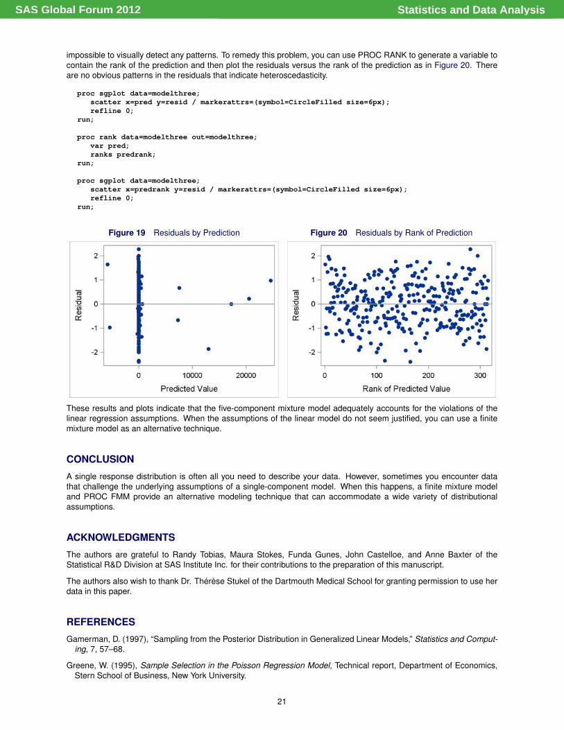
impossible to visually detect any patterns. To remedy this problem, you can use PROC RANK to generate a variable tocontain the rank of the prediction and then plot the residuals versus the rank of the prediction as in Figure 20. Thereare no obvious patterns in the residuals that indicate heteroscedasticity.

proc sgplot data=modelthree;scatter x=pred y=resid / markerattrs=(symbol=CircleFilled size=6px);refline 0;

run;

proc rank data=modelthree out=modelthree;var pred;ranks predrank;

run;

proc sgplot data=modelthree;scatter x=predrank y=resid / markerattrs=(symbol=CircleFilled size=6px);refline 0;

run;

Figure 19 Residuals by Prediction Figure 20 Residuals by Rank of Prediction

These results and plots indicate that the five-component mixture model adequately accounts for the violations of thelinear regression assumptions. When the assumptions of the linear model do not seem justified, you can use a finitemixture model as an alternative technique.

CONCLUSION

A single response distribution is often all you need to describe your data. However, sometimes you encounter datathat challenge the underlying assumptions of a single-component model. When this happens, a finite mixture modeland PROC FMM provide an alternative modeling technique that can accommodate a wide variety of distributionalassumptions.

ACKNOWLEDGMENTS

The authors are grateful to Randy Tobias, Maura Stokes, Funda Gunes, John Castelloe, and Anne Baxter of theStatistical R&D Division at SAS Institute Inc. for their contributions to the preparation of this manuscript.

The authors also wish to thank Dr. Thérèse Stukel of the Dartmouth Medical School for granting permission to use herdata in this paper.

REFERENCES

Gamerman, D. (1997), “Sampling from the Posterior Distribution in Generalized Linear Models,” Statistics and Comput-ing, 7, 57–68.

Greene, W. (1995), Sample Selection in the Poisson Regression Model, Technical report, Department of Economics,Stern School of Business, New York University.

21


Lambert, D. (1992), “Zero-Inflated Poisson Regression Models with an Application to Defects in Manufacturing,” Tech-nometrics, 34, 1–14.

Long, J. S. (1997), Regression Models for Categorical and Limited Dependent Variables, Thousand Oaks, CA: SagePublications.

McLachlan, G. J. and Basford, K. E. (1988), Mixture Models, New York: Marcel Dekker.

Mullahy, J. (1986), “Specification and Testing of Some Modified Count Data Models,” Journal of Econometrics, 33,341–365.

Nierenberg, D., Stukel, T., Baron, J., Dain, B., and Greenberg, E. (1989), “Determinants of plasma levels of beta-carotene and retinol. Skin Cancer Prevention Study Group.” American Journal of Epidemiology, 130, 511–21.

Schlattmann, P. (2009), Medical Applications of Finite Mixture Models, Springer Verlag.

Stukel, T. (2008), “Determinants of Plasma Retinol and Beta-Carotene Levels,” StatLib Datasets Archive.URL http://lib.stat.cmu.edu/datasets/Plasma_Retinol

Symons, M. J., Grimson, R. C., and Yuan, Y. C. (1983), “Clustering of Rare Events,” Biometrics, 39, 193–205.

CONTACT INFORMATION

Dave KesslerSAS Institute Inc.SAS Campus DriveCary, NC, [email protected]

Allen McdowellSAS Institute Inc.SAS Campus DriveCary, NC, [email protected]

SAS and all other SAS Institute Inc. product or service names are registered trademarks or trademarks of SAS InstituteInc. in the USA and other countries. ® indicates USA registration.

Other brand and product names are trademarks of their respective companies.

22


http://lib.stat.cmu.edu/datasets/Plasma_Retinol

328-2012: Introducing the FMM Procedure for Finite … the FMM Procedure for Finite Mixture Models...

Documents

Transcript of 328-2012: Introducing the FMM Procedure for Finite … the FMM Procedure for Finite Mixture Models...