3.2, 3.3 Inverting Matrices P. Danziger Properties of...
22
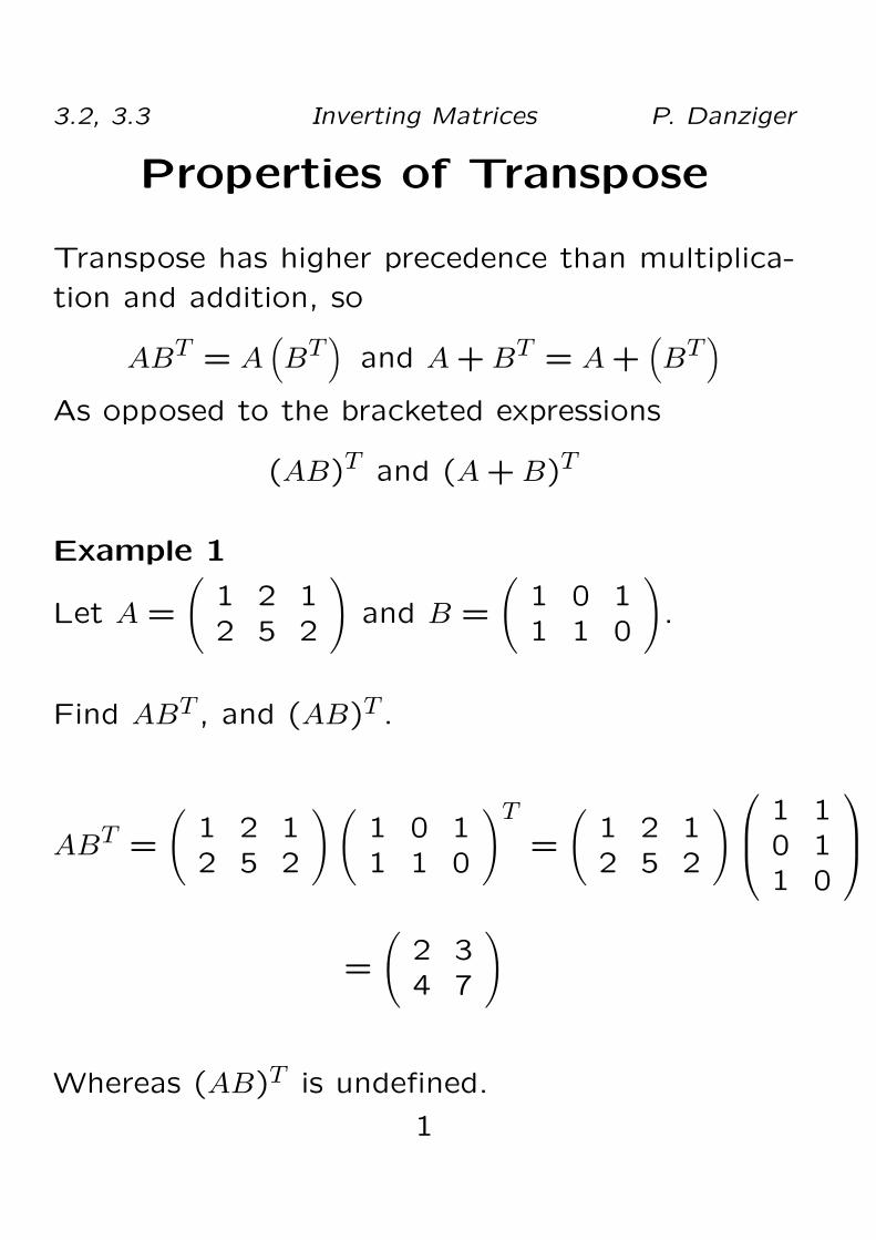
3.2, 3.3 Inverting Matrices P. Danziger Properties of Transpose Transpose has higher precedence than multiplica- tion and addition, so AB T = A B T and A + B T = A + B T As opposed to the bracketed expressions (AB ) T and (A + B ) T Example 1 Let A = 1 2 1 2 5 2 ! and B = 1 0 1 1 1 0 ! . Find AB T , and (AB ) T . AB T = 1 2 1 2 5 2 ! 1 0 1 1 1 0 ! T = 1 2 1 2 5 2 ! 1 1 0 1 1 0 = 2 3 4 7 ! Whereas (AB ) T is undefined. 1
-
Upload
vuongduong -
Category
Documents
-
view
218 -
download
0
Transcript of 3.2, 3.3 Inverting Matrices P. Danziger Properties of...
3.2, 3.3 Inverting Matrices P. Danziger
Properties of Transpose
Transpose has higher precedence than multiplica-
tion and addition, so
ABT = A(BT
)and A+BT = A+
(BT
)As opposed to the bracketed expressions
(AB)T and (A+B)T
Example 1
Let A =
(1 2 12 5 2
)and B =
(1 0 11 1 0
).
Find ABT , and (AB)T .
ABT =
(1 2 12 5 2
)(1 0 11 1 0
)T=
(1 2 12 5 2
) 1 10 11 0
=
(2 34 7
)
Whereas (AB)T is undefined.
1

3.2, 3.3 Inverting Matrices P. Danziger
Theorem 2 (Properties of Transpose) Given ma-
trices A and B so that the operations can be pre-
formed
1. (AT )T = A
2. (A+B)T = AT +BT and (A−B)T = AT −BT
3. (kA)T = kAT
4. (AB)T = BTAT
2

3.2, 3.3 Inverting Matrices P. Danziger
Matrix AlgebraTheorem 3 (Algebraic Properties of Matrix Multiplication)
1. (k + `)A = kA + `A (Distributivity of scalar
multiplication I)
2. k(A + B) = kA + kB (Distributivity of scalar
multiplication II)
3. A(B+C) = AB+AC (Distributivity of matrix
multiplication)
4. A(BC) = (AB)C (Associativity of matrix mul-
tiplication)
5. A + B = B + A (Commutativity of matrix ad-
dition)
6. (A + B) + C = A + (B + C) (Associativity of
matrix addition)
7. k(AB) = A(kB) (Commutativity of Scalar Mul-
tiplication)
3
3.2, 3.3 Inverting Matrices P. Danziger
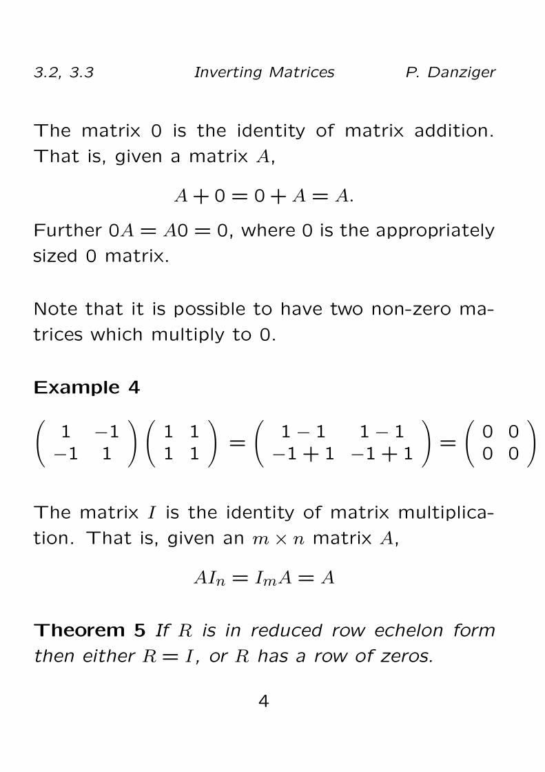
The matrix 0 is the identity of matrix addition.
That is, given a matrix A,
A+ 0 = 0 +A = A.
Further 0A = A0 = 0, where 0 is the appropriately
sized 0 matrix.
Note that it is possible to have two non-zero ma-
trices which multiply to 0.
Example 4(1 −1−1 1
)(1 11 1
)=
(1− 1 1− 1−1 + 1 −1 + 1
)=
(0 00 0
)
The matrix I is the identity of matrix multiplica-
tion. That is, given an m× n matrix A,
AIn = ImA = A
Theorem 5 If R is in reduced row echelon form
then either R = I, or R has a row of zeros.
4

3.2, 3.3 Inverting Matrices P. Danziger
Theorem 6 (Power Laws) For any square ma-trix A,
ArAs = Ar+s and (Ar)s = Ars
Example 7
1. 0 0 1
1 0 12 2 0
4
=
0 0 1
1 0 12 2 0
2
2
2. Find A6, where
A =
(1 01 1
)
A6 = A2A4 = A2(A2)2
.
Now A2 =
(1 02 1
), so
A2(A2)2
=
(1 02 1
)(1 02 1
)2
=
(1 02 1
)(1 03 1
)
=
(1 05 1
)
5
3.2, 3.3 Inverting Matrices P. Danziger
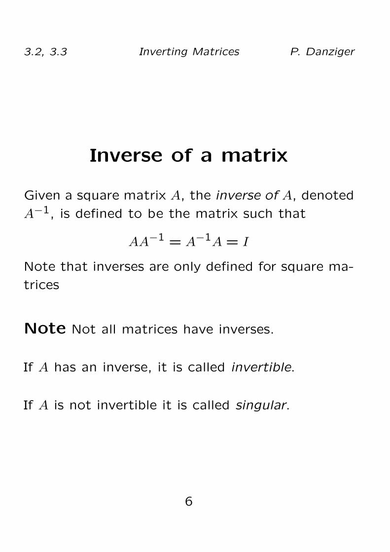
Inverse of a matrix
Given a square matrix A, the inverse of A, denoted
A−1, is defined to be the matrix such that
AA−1 = A−1A = I
Note that inverses are only defined for square ma-
trices
Note Not all matrices have inverses.
If A has an inverse, it is called invertible.
If A is not invertible it is called singular.
6

3.2, 3.3 Inverting Matrices P. Danziger
Example 8
1. A =
(1 22 5
)A−1 =
(5 −2−2 1
)
Check:
(1 22 5
)(5 −2−2 1
)=
(1 00 1
)
2. A =
(1 22 4
)Has no inverse
3. A =
1 1 11 2 11 1 2
A−1 =
3 −1 −1−1 1 0−1 0 1
Check:
1 1 11 2 11 1 2
3 −1 −1−1 1 0−1 0 1
=
1 0 00 1 00 0 1
4. A =
1 2 12 1 33 3 4
Has no inverse
7
3.2, 3.3 Inverting Matrices P. Danziger
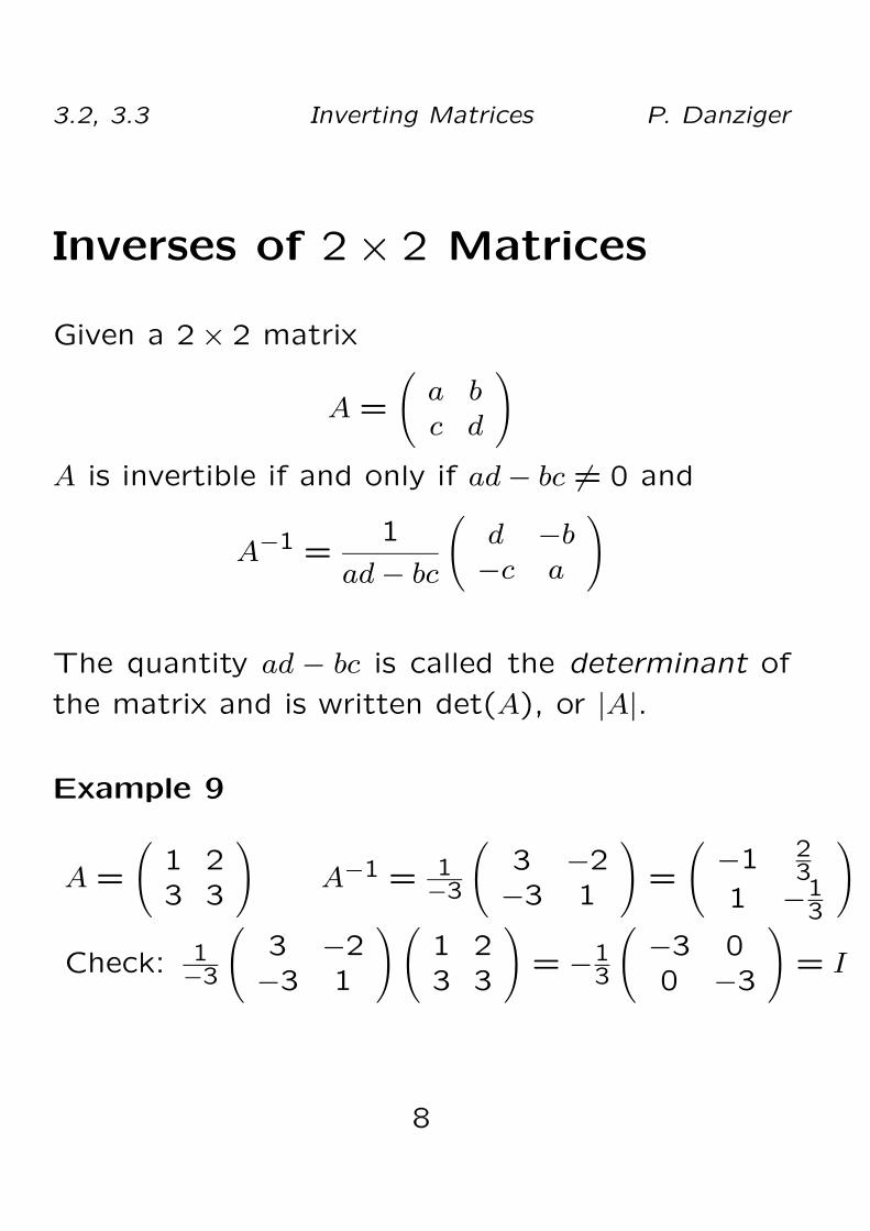
Inverses of 2× 2 Matrices
Given a 2× 2 matrix
A =
(a bc d
)A is invertible if and only if ad− bc 6= 0 and
A−1 =1
ad− bc
(d −b−c a
)
The quantity ad − bc is called the determinant of
the matrix and is written det(A), or |A|.
Example 9
A =
(1 23 3
)A−1 = 1
−3
(3 −2−3 1
)=
(−1 2
31 −1
3
)
Check: 1−3
(3 −2−3 1
)(1 23 3
)= −1
3
(−3 00 −3
)= I
8
3.2, 3.3 Inverting Matrices P. Danziger
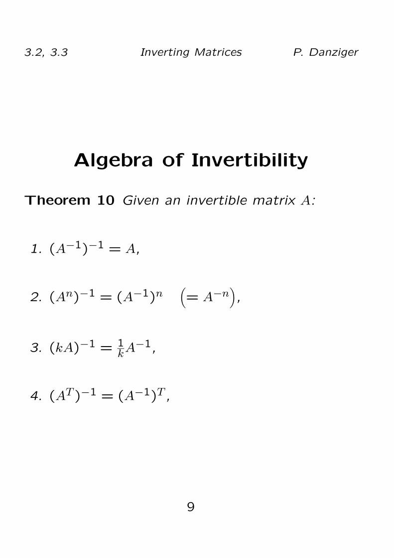
Algebra of Invertibility
Theorem 10 Given an invertible matrix A:
1. (A−1)−1 = A,
2. (An)−1 = (A−1)n(= A−n
),
3. (kA)−1 = 1kA−1,
4. (AT )−1 = (A−1)T ,
9

3.2, 3.3 Inverting Matrices P. Danziger
Theorem 11 Given two invertible matrices A and
B
(AB)−1 = B−1A−1.
Proof: Let A and B be invertible matricies and
let C = AB, so C−1 = (AB)−1.
Consider C = AB.
Multiply both sides on the left by A−1:
A−1C = A−1AB = B.
Multiply both sides on the left by B−1.
B−1A−1C = B−1B = I.
So, B−1A−1 is the matrix you need to multiply C
by to get the identity.
Thus, by the definition of inverse
B−1A−1 = C−1 = (AB)−1.
10

3.2, 3.3 Inverting Matrices P. Danziger
A Method for Inverses
Given a square matrix A and a vector b ∈ Rn,
consider the equation
Ax = b
This represents a system of equations with coeffi-
cient matrix A.
Multiply both sides by A−1 on the left, to get
A−1Ax = A−1b.
But A−1A = In and Ix = x, so we have
x = A−1b.
Note that we have a unique solution. The as-
sumption that A is invertible is equaivalent to the
assumption that Ax = b has unique solution.
11

3.2, 3.3 Inverting Matrices P. Danziger
During the course of Gauss-Jordan elimination on
the augmented matrix (A|b) we reduce A→ I and
b→ A−1b, so (A|b)→(I|A−1b
).
If we instead augment A with I, row reducing will
produce (hopefully) I on the left and A−1 on the
right, so (A|I)→(I|A−1
).
The Method:
1. Augment A with I
2. Use Gauss-Jordan to obtain (I|A−1) .
3. If I does not appear on the left, A is not in-
vertable.
Otherwise, A−1 is given on the right.
12

3.2, 3.3 Inverting Matrices P. Danziger
Example 12
1. Find A−1, where
A =
1 2 32 5 53 5 8
13
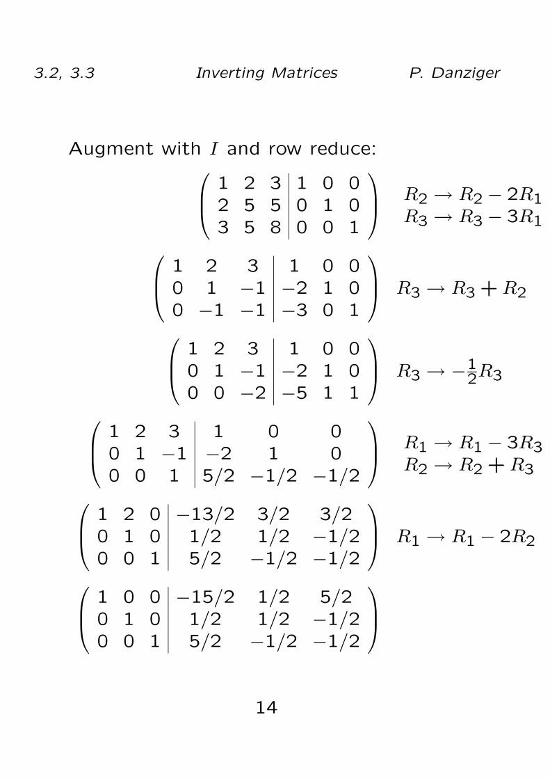
3.2, 3.3 Inverting Matrices P. Danziger
Augment with I and row reduce: 1 2 3 1 0 02 5 5 0 1 03 5 8 0 0 1
R2 → R2 − 2R1R3 → R3 − 3R1
1 2 3 1 0 00 1 −1 −2 1 00 −1 −1 −3 0 1
R3 → R3 +R2
1 2 3 1 0 00 1 −1 −2 1 00 0 −2 −5 1 1
R3 → −12R3
1 2 3 1 0 00 1 −1 −2 1 00 0 1 5/2 −1/2 −1/2
R1 → R1 − 3R3R2 → R2 +R3
1 2 0 −13/2 3/2 3/20 1 0 1/2 1/2 −1/20 0 1 5/2 −1/2 −1/2
R1 → R1 − 2R2
1 0 0 −15/2 1/2 5/20 1 0 1/2 1/2 −1/20 0 1 5/2 −1/2 −1/2
14

3.2, 3.3 Inverting Matrices P. Danziger
So
A−1 =1
2
−15 1 51 1 −15 −1 −1
To check inverse multiply together:
AA−1 =
1 2 32 5 53 5 8
12
−15 1 51 1 −15 −1 −1
= 1
2
2 0 00 2 00 0 2
= I
2. Solve Ax = b in the case where b = (2,2,4)T .
x = A−1b = 12
−15 1 51 1 −15 −1 −1
2
24
= 1
2
−1804
=
−902
15

3.2, 3.3 Inverting Matrices P. Danziger
3. Solve Ax = b in the case where b = (2,0,2)T .
x = A−1b = 12
−15 1 51 1 −15 −1 −1
2
02
= 1
2
−2008
=
−904
4. Give a solution to Ax = b in the general case
where b = (b1, b2, b3)
x = 12
−15 1 51 1 −15 −1 −1
b1b2b3
= 1
2
−15b1 + b2 + 5b3b1 + b2 − b35b1 − b2 − b3
16
3.2, 3.3 Inverting Matrices P. Danziger
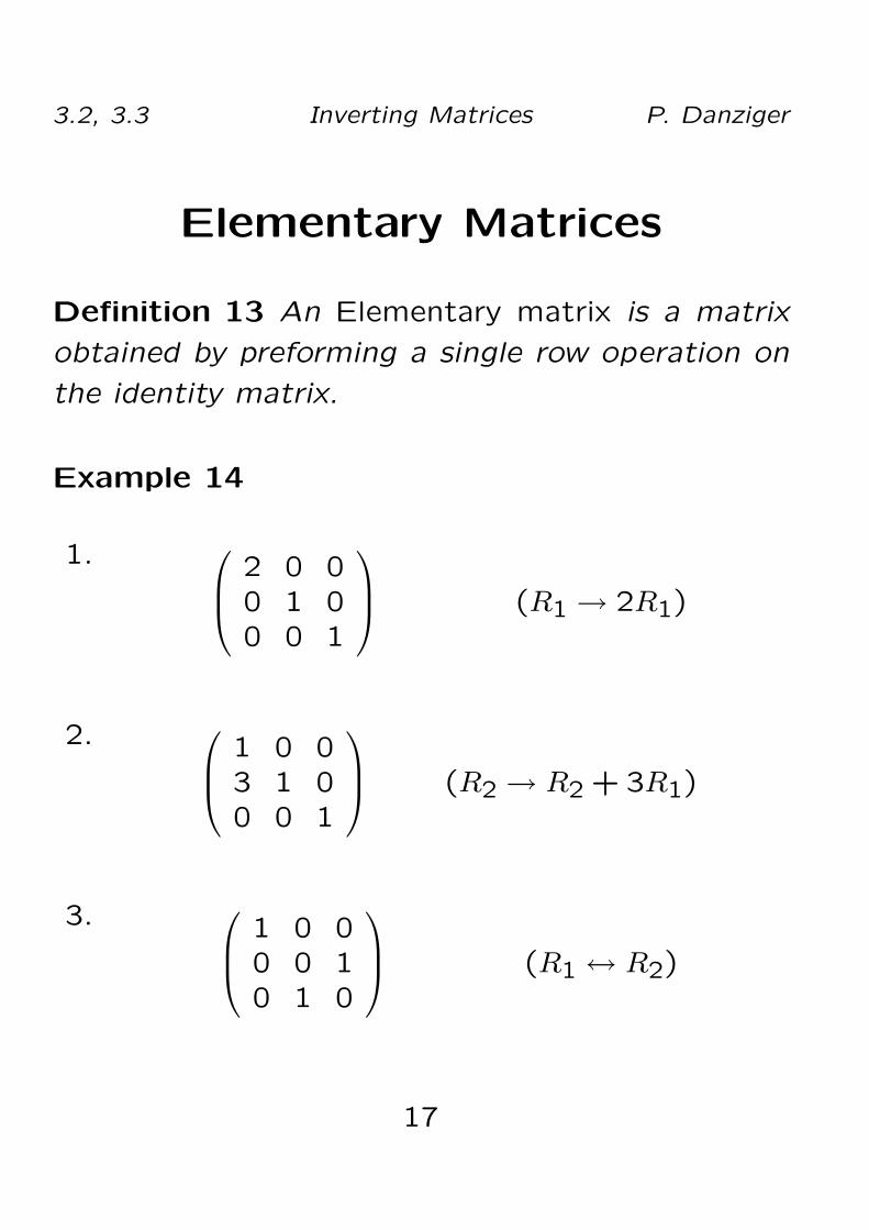
Elementary Matrices
Definition 13 An Elementary matrix is a matrix
obtained by preforming a single row operation on
the identity matrix.
Example 14
1. 2 0 00 1 00 0 1
(R1 → 2R1)
2. 1 0 03 1 00 0 1
(R2 → R2 + 3R1)
3. 1 0 00 0 10 1 0
(R1 ↔ R2)
17

3.2, 3.3 Inverting Matrices P. Danziger
Theorem 15 If E is an elementary matrix ob-
tained from Im by preforming the row operation R
and A is any m× n matrix, then EA is the matrix
obtained by preforming the same row operation R
on A.
Example 16
A =
1 1 12 1 03 2 1
1. 2 0 0
0 1 00 0 1
1 1 1
2 1 03 2 1
=
2 2 22 1 03 2 1
∼ 2R2 on A
2. 1 0 03 1 00 0 1
1 1 1
2 1 03 2 1
=
1 1 15 4 33 2 1
∼ R2 → R2 + 3R1on A
3.
18

3.2, 3.3 Inverting Matrices P. Danziger 1 0 00 0 10 1 0
1 1 1
2 1 03 2 1
=
1 1 13 2 12 1 0
∼ R2 ↔ R3on A
Inverses of Elementary Matrices
If E is an elementary matrix then E is invertible and
E−1 is an elementary matrix corresponding to the
row operation that undoes the one that generated
E. Specifically:
• If E was generated by an operation of the form
Ri → cRi then E−1 is generated by Ri → 1cRi.
• If E was generated by an operation of the form
Ri → Ri + cRj then E−1 is generated by
Ri → Ri − cRj.
• If E was generated by an operation of the form
Ri ↔ Rj then E−1 is generated by Ri ↔ Rj.
19

3.2, 3.3 Inverting Matrices P. Danziger
Example 17
1. E =
2 0 00 1 00 0 1
E−1 =
12 0 00 1 00 0 1
2. E =
1 0 03 1 00 0 1
E−1 =
1 0 0−3 1 00 0 1
3. E =
1 0 00 0 10 1 0
E−1 = E
20

3.2, 3.3 Inverting Matrices P. Danziger
Elementary Matricies and Solv-ing EquationsConsider the steps of Gauss Jordan elimination to
find the solution to a system of equations Ax = b.
This consists of a series of row operations, each
of which is equivalent to multiplying on the left by
an elementary matrix Ei.
AEle. row ops.−−− −→ B,
Where B is the RREF of A.
So EkEk−1 . . . E2E1A = B for some appopriately
defined elementary matrices E1 . . . Ek.
Thus A = E−11 E−1
2 . . . E−1k−1E
−1k B
Now if B = I (so the RREF of A is I), thenA = E−1
1 E−12 . . . E−1
k−1E−1k
and A−1 = EkEk−1 . . . E2E1
Theorem 18 A is invertable if and only if it is the
product of elementary matrices.
21

3.2, 3.3 Inverting Matrices P. Danziger
Summing Up Theorem
Theorem 19 (Summing up Theorem Version 1)
For any square n × n matrix A, the following are
equivalent statements:
1. A is invertible.
2. The RREF of A is the identity, In.
3. The equation Ax = b has unique solution
(namely x = A−1b).
4. The homogeneous system Ax = 0 has only the
trivial solution (x = 0)
5. The REF of A has exactly n pivots.
6. A is the product of elementary matrices.
22